Optimization algorithm for minimizing railway energy consumption in hybrid powertrain architectures: A direct method approach using a novel two-dimensional efficiency map approximation

Abstract

SEnSOR (Smart Energy Speed Optimizer Rail) is a direct method based optimization algorithm developed at DLR for determining minimum energy speed trajectories for railway vehicles. This paper aims to reduce model error and improve this algorithm for any alternative powertrain architecture. Model simplifications such as projecting the efficiency maps of different train components onto one-dimensional space can lead to inaccuracies and non-optimalities in reality. In this work, 2D section-wise Chua functional representation was used to capture the complete behavior of efficiency maps and discuss its benefits. For this purpose, a new smoothing method was developed. It was observed that there is an average of 6% error in the energy calculation when both, 1D and 2D, models are compared against each other. Previously, solving for different powertrain architectures was time consuming with the requirement of manual modifications to the optimization problem. With a modular approach, the algorithm was modified to flexibly adapt the problem formulation to automatically take into account any changes in powertrain architectures with minimum user input. The benefit is demonstrated by performing optimization on a bi-mode train with three different power sources as developed within the EU-project FCH2RAIL. The advanced algorithm is now capable to adapt to such complex architectures and provide feasible optimization results within a reasonable time.

Introduction

Compared to diesel engines, electric motors are more efficient, require less maintenance and allow for more environmental-friendly operation of railway. Thus, diesel-powered trains which previously covered non-electrified railway sections are more and more replaced by electric solutions. If overhead line electrification is not an option due to economic or technical constraints, train architectures with onboard energy storage are required. Currently, different topologies are being developed, for example consisting of batteries, fuel cells, capacitors and sometimes additional overhead line power supply. ¹

Even with electrified operation, there is still a need to reduce energy demand and corresponding costs, as the transformation to sustainable power supply requires heavily increased amounts of renewable electricity and green hydrogen in all sectors. ² Thus, to reduce energy demand in railway transport, Scheepmaker et al. ³ highlight four main approaches: minimum energy train control, energy-efficient timetabling, efficient components and demand analysis. Focusing on optimal control, they found Pontryagin’s Maximum Principle (PMP) to be intensively applied to determine energy-efficient train operation regimes. The optimal switching points between these regimes and hence the optimal trajectory are then usually obtained by other numerical algorithms such as Gradient Search, Dynamic Programming (DP) or Genetic Algorithms. The application of Direct Methods (DM) to such problems is still rare in the literature.

Macian et al. ⁴ found that using DM for combined energy management and trajectory optimization on a diesel-electric train yields similar results in comparison to that obtained by DP and PMP, while requiring heavily reduced computational time and memory. This motivated the development of SEnSOR (Smart Energy & Speed Optimizer Rail) for combined offline energy management and speed profile optimization of hybrid electric trains. Schenker et al. ⁵ and Kühlkamp et al. ⁶ extended the method to battery and fuel cell electric trains and improved upon the approach of Macian et al. by including detailed train models and flexible handling of electrification patterns in their optimization tool SEnSOR.

The following paper poses the question if SEnSOR is able to handle any kind of electric power train architecture in a flexible and straight-forward manner. At the same time, it aims to demonstrate that utilizing the possibility of DM to include high-complexity constraints enables us to reduce model inaccuracies significantly. It is expected that the gains in flexibility and model accuracy will increase the overall computational time taken by the algorithm. However, this paper shows that the benefits may outweigh this aspect.

The first section provides a brief overview of the current algorithm and its implementation objectives. Afterwards the models and implementation methods are described in detail, including the derivation of our 2D efficiency map smoothing method. The subsequent section illustrates and discusses example results, concluding with the most significant findings.

Background - The SEnSOR algorithm

SEnSOR is a DM-based optimization algorithm for calculating minimum energy trajectory for various railway vehicles, implemented in MATLAB. In particular, it optimizes speed profile and energy management simultaneously to guarantee a tailored solution for a given train type. It automatically transforms a standardized input of vehicle and track parameters into objective functions, nonlinear constraints and boundary conditions of the optimization. To find the mathematical optimum, SEnSOR uses an interface for IPOPT (Interior Point OPTimizer), ⁷ which implements interior point line search filter method to find a local solution of a nonlinear optimization problem.

With its current capabilities, ⁶ SEnSOR still faces challenges to account for all realistic features. Most importantly, it uses simplified 1D load-dependent efficiency characteristics for all components. For some of them however, the efficiency has a significant dependency on more than power throughput, for example speed. This simplification can cause inaccuracies. An optimized control obtained by this model can be non-optimal in reality, if used directly. Shifting to a multidimensional model may prove computationally expensive. In this study, we will try to answer what is the benefit of transitioning to such a more realistic model by performing simulations on a test track.

Secondly, SEnSOR shall be flexible to account for any changes in components or the entire train architecture. Currently, each time a change is to be made, the optimal control problem (OCP) has to be manually reformulated. This can be very time consuming and sometimes lead to model and human-induced errors. For this study, we will remove the requirement of hard-coding the optimization problem by the user, introduce additional modularity into SEnSOR’s implementation and analyze its benefits. To demonstrate the adaptability to different train architectures, we will then optimize the energy management control of a complex bi-mode powertrain architecture. This is part of the FCH2RAIL project, ⁸ in which this novel train type is developed and tested. One of the goals within the project is to optimize the energy management strategy of the bi-mode train to reduce energy consumption, both electric and hydrogen. In this paper, this was done by running simulations using a generic train model on a long real world track.

Models and methods

Two-Dimensional modeling of efficiency maps

The objective function and constraints of the OCP in SEnSOR comprises of functions that use the efficiency maps of different train components. These maps are often available in the form of two-dimensional numerical tables, that is, values of efficiency at discrete values of wheel speeds and power control settings. In SEnSOR, this map was to be modified to compute the power loss of the component by taking the normalized power p and the speed of the train v as input arguments to directly give the normalized power as output. It is now a choice how one chooses to handle the discrete data. One natural idea would be to use them by interpolation. However, IPOPT requires that the objective functions and constraints are at least twice continuously differentiable to guarantee the local optimality of the solution. In order to incorporate them into the objective function and constraints and solve the problem using IPOPT, these maps were to be represented by an explicit analytical function, $f:{\mathbb{R}}^2\to \mathbb{R}$ such that f ∈ C². Having an explicit form that fits the given data can prove to be more convenient than using a higher order interpolation as it is less computationally expensive and enables to perform standard mathematical operations on them.

For simplification, the task was previously reduced to finding an approximation of f (p, v), $\widehat{f}:\mathbb{R}\to \mathbb{R}$ , by averaging the values of efficiency along the dimension of speed, using one-dimensional canonical piecewise-linear models, developed by Chua and Kang. ⁹ This model is equivalent to a 1D linear interpolation, but has a compact mathematical representation. A smoothing procedure to ensure differentiability of such models was developed by Jimenez-Fernandez et al. ¹⁰ The combination of both appear to be far more performant than any state of the art interpolation methods with the added benefit of providing an analytical representation of the data. By using these methods, the required function can be represented as follows:

$\widehat{f}\left(P\right)=A+BP+{\displaystyle \sum }_{j=1}^{{\sigma }_P}C\hspace{0.17em}\ln \left(1+e^{-{\alpha }_{pj}\left(P-{\beta }_{pj}\right)}\right)$

(1)

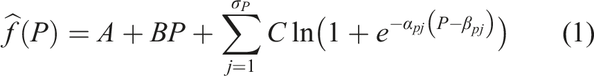
Where β _pj ’s and α _pj ’s are the breakpoints and the smoothing parameters that control the level of smoothing at each breakpoint in the P-direction, σ _p is the total number of breakpoints, A, B and C are data-dependent model coefficients. Thus, the objective function and constraints of the OCP were effectively reduced to be only dependent on the train power control setting.

While this procedure simplifies the problem and results in a robust solution, it introduces a significant model error in the energy transmission between different train components. The effect of averaging of efficiencies may under/over-estimate the power losses depending on the available data and thus cause inaccuracies in the final solution. An optimal control solution using such a simplified model can be non-optimal with realistic energy transmission. Thus, it may be crucial to consider the multidimensional dependence of efficiencies. We will analyze and discuss the benefits and drawbacks of shifting to a more realistic implementation. For this, an explicit 2D function f is required as detailed above.

Chua and Kang ⁹ developed a section-wise piecewise-linear models to also fit multi-dimensional data. In this case, 1D canonical piecewise-linear representation were used in each dimension by fixing the other dimensions. This is mathematically equivalent to a bilinear interpolation in 2D with the additional benefit of having a compact analytical representation of the given 2D data. However, unlike the 1D case, there exists no formal smoothing procedure for such a model. In this study, we extend the work of Jimenez-Fernandez et al. ¹⁰ by deriving a transformation formula for smoothing 2D section-wise piecewise-linear functions.

Smoothing method for functional 2D-Representations

The section-wise piecewise-linear representation of a given 2D dataset is obtained by using a 1D chua piecewise linear representation in one dimension, while holding the other dimension fixed.

$\begin{array}{ll}f\left(x,y\right)& =a_1+b_{1}y+{\displaystyle \sum }_{i=1}^{{\sigma }_y}{c}_{1i}\left|y-{\beta }_{yi}\right|\\ & +\left(a_2+b_{2}y+{\displaystyle \sum }_{i=1}^{{\sigma }_y}{c}_{2i}\left|y-{\beta }_{yi}\right|\right)x\\ & +{\displaystyle \sum }_{j=1}^{{\sigma }_x}\left(a_{3j}+b_{3j}y+{\displaystyle \sum }_{i=1}^{{\sigma }_y}{c}_{3ij}\left|y-{\beta }_{yi}\right|\right)\left|x-{\beta }_{xj}\right|\end{array}$

(2)

where β _x j’s and β _y i’s are the breakpoints in x-direction and y-direction respectively, and σ _x and σ _y represent the total number of such points in each direction. Given the data points, the coefficients {a₁, b₁, c_1i, a₂, b₂, c_2i, a_3j, b_3j, c_3ij}, are determined by solving a system of linear equations. ⁹

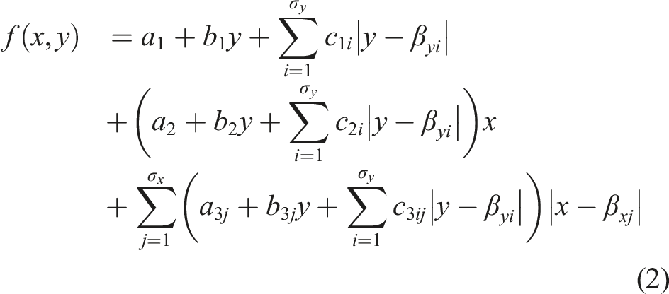
Twice continuous differentiability of this function is ensured by applying a smooth approximation of the absolute value terms. ¹⁰ For the detailed derivation of the transformation formula, see the Supplementary Material. For clarity, the final transformation formula is re-written:

$\begin{array}{ll}\widehat{f}\left(x,y\right)& =A_1+B_{1}y+{\displaystyle \sum }_{i=1}^{{\sigma }_y}{C}_{1i}\hspace{0.17em}\ln \left(1+e^{-{\alpha }_{yi}\left(y-{\beta }_{yi}\right)}\right)\\ & +\left(A_2+B_{2}y+{\displaystyle \sum }_{i=1}^{{\sigma }_y}{C}_{2i}\hspace{0.17em}\ln \left(1+e^{-{\alpha }_{yi}\left(y-{\beta }_{yi}\right)}\right)\right)x\\ & +{\displaystyle \sum }_{j=1}^{{\sigma }_x}\left(A_{3j}+B_{3j}y+{\displaystyle \sum }_{i=1}^{{\sigma }_y}{C}_{3ij}\hspace{0.17em}\ln \left(1+e^{-{\alpha }_{yi}\left(y-{\beta }_{yi}\right)}\right)\right)\\ & \hspace{0.17em}\ln \left(1+e^{-{\alpha }_{xj}\left(x-{\beta }_{xj}\right)}\right)\end{array}$

(3)

where, {A₁, B₁, C_1i, A₂, B₂, C_2i, A_3j, B_3j, C_3ij} can be defined as the parameters of the 2D piecewise smoothed function as follows:

$\begin{array}{l}{A}_1=a_1-{\displaystyle \sum }_{i=1}^{{\sigma }_y}{c}_{1i}{\beta }_{1i}-{\displaystyle \sum }_{j=1}^{{\sigma }_x}\left(a_{3j}-{\displaystyle \sum }_{i=1}^{{\sigma }_y}{c}_{3ij}{\beta }_{yi}\right){\beta }_{xj}\\ A_2=a_2-{\displaystyle \sum }_{i=1}^{{\sigma }_y}{c}_{2i}{\beta }_{yi}+{\displaystyle \sum }_{j=1}^{{\sigma }_x}\left(a_{3j}-{\displaystyle \sum }_{i=1}^{{\sigma }_y}{c}_{3ij}{\beta }_{yi}\right)\\ A_{3j}=\frac{2}{{\alpha }_{xj}}\left(a_{3j}-{\displaystyle \sum }_{i=1}^{{\sigma }_y}{c}_{3ij}{\beta }_{yi}\right)\\ B_1=b_1+{\displaystyle \sum }_{i=1}^{{\sigma }_y}{c}_{1i}-{\displaystyle \sum }_{j=1}^{{\sigma }_x}\left(b_{3j}+{\displaystyle \sum }_{i=1}^{{\sigma }_y}{c}_{3ij}\right){\beta }_{xj}\\ B_2=b_2+{\displaystyle \sum }_{i=1}^{{\sigma }_y}{c}_{2i}+{\displaystyle \sum }_{j=1}^{{\sigma }_x}\left(b_{3j}+{\displaystyle \sum }_{i=1}^{{\sigma }_y}{c}_{3ij}\right)\\ B_{3j}=\frac{2}{{\alpha }_{xj}}\left(b_{3j}+{\displaystyle \sum }_{i=1}^{{\sigma }_y}{c}_{3ij}\right)\\ C_{1i}={\displaystyle \sum }_{i=1}^{{\sigma }_y}\frac{2}{{\alpha }_{yi}}\left(c_{1i}-{\displaystyle \sum }_{j=1}^{{\sigma }_x}{c}_{3ij}{\beta }_{xj}\right)\\ C_{2i}={\displaystyle \sum }_{i=1}^{{\sigma }_y}\frac{2}{{\alpha }_{yi}}\left(c_{1i}+{\displaystyle \sum }_{j=1}^{{\sigma }_x}{c}_{3ij}\right)\\ C_{3ij}=\frac{4c_{3ij}}{{\alpha }_{yi}{\alpha }_{xj}}\text{where},i=1,\dots ,{\sigma }_y,j=1,\dots ,{\sigma }_x\end{array}$

(4)

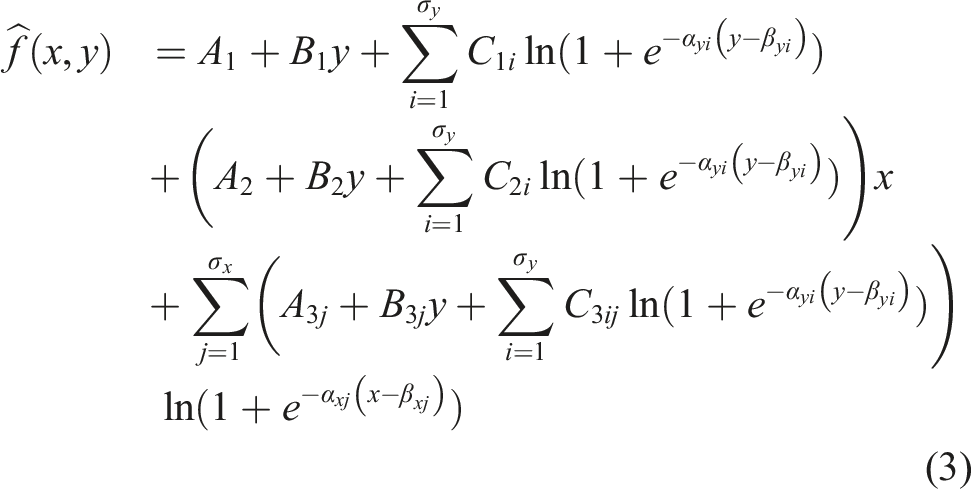
The parameters α control the smoothness of the function at breakpoints, that is how much the function deviates from the specified breakpoint. More formally, like in the 1D case, ¹⁰ we can state the following theorem:

Theorem 1

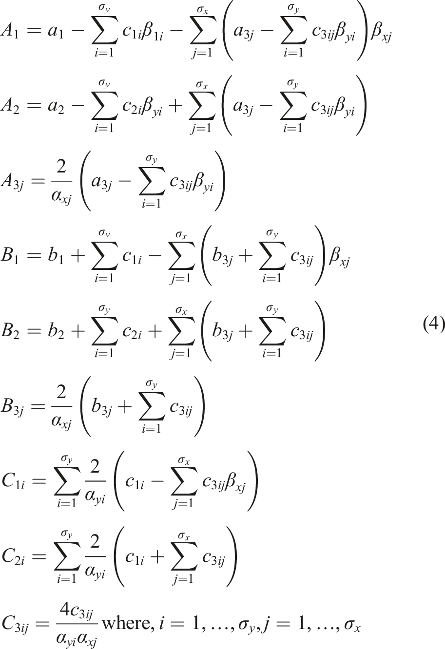
Any two-dimensional canonical section-wise piecewise linear function that is characterized by σ _x and σ _y breakpoints, respectively in each direction, can be transformed into a section-wise linear smooth-piecewise function expressed as in eq. (3), where the set of (σ _x σ _y + 2σ _x + 2σ _y + 4) parameters can be determined with eqns. (4) and the (σ _y + σ _x ) parameters {α _xj , α _yi } for i ∈ [σ _y ] and j ∈ [σ _x ] can be used to preserve a smoothness at any breakpoint location. As the values of α approach ∞, eq. (3) approaches eq. (2).

For a detailed proof of this theorem, see the Supplemental Material provided. In the next subsection, we discuss how a suitable smoothing parameter was choosen to construct these smoothed functions for our objective functions and constraints.

Implementation

From Theorem, 1 it is clear that we need to choose the smoothing parameters as high as possible to reduce the approximation error with the data points. However, with increasing values of the smoothing parameters α _i there is a reduction in function smoothness. We already discussed that IPOPT requires the objective and constraints to be at least twice continuously differentiable. Therefore, it is essential to choose a smoothing parameter that is sufficiently big to have a low approximation error, but at the same time not too big, such that the functions and their derivatives, in particular the second derivative, do not exist and are unbounded. The following algorithm was implemented to do this task efficiently.

Algorithm 1: Smoothing 2D section-wise canonical piecewise-linear functions

Input: Dataset, $\mathcal{D}=\left(P_{\widehat{j}},v_{\widehat{i}},P_{out-\widehat{k}}\right)$ for $\widehat{i}=1,\dots ,{\sigma }_v+2$ , $\widehat{j}=1,\dots ,{\sigma }_P+2$ , $\widehat{k}=1,\dots ,\left({\sigma }_P+2\right)\left({\sigma }_v+2\right)$

Output: $\widehat{f}$

1 compute {A1, A2, A3j, B1, B2, B3j, C1i, C2i, C3ij} from equation (4) for i = 1, …, σ v , j = 1, …, σ P

2 Initialize α Pj , α vi = 10000

3 while $N:=\left\{{\partial }_{PP}\widehat{f}\left(P,v\right),{\partial }_{Pv}\widehat{f}\left(P,v\right),{\partial }_{vv}\widehat{f}\left(P,v\right)\right\}$ are unbounded or are not defined do

4 determine i’s and j’s that make elements of N not defined

5 α Pj = 0.99α Pj , α vi = 0.99α vi for i’s and j’s from step 4

6 compute $\widehat{f}$ with updated values of α Pj ’s and α vi ’s

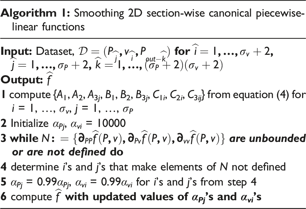
The fourth step of the algorithm can be efficiently done by identifying the terms inside the different summations in equation (3), whose second derivatives are unbounded or are not defined. The value of α _i are chosen in such a way that these derivative terms remain well-defined and bounded at any given point. The choice of α _i depends on the distance between the point of interest and the breakpoints. Since the terms to approximate each piecewise-linear sections of the whole functions are either monotonously in- or decreasing, the critical values are on the boundary of the domain. Hence, it is most efficient to check only at boundaries if the derivative terms are defined and lower the respective α if they are not.

Modular, flexible power train architecture

Following the approach to a more realistic representation of the system, the next step after modeling the efficiencies in a 2D-manner is to depict all components more realistically. The previous implementation ⁶ represented the train architectures in a hard-coded way within the constraints and objective functions. As long as the power train architecture is exactly the same as in this representation, no model error will occur. However, if the train architecture or the type of some of the components changes, either the model has to be adapted within the code or a simplified approximation to fit the current model has to be made which introduces an additional model error. To avoid this, the tool was revised to account for a flexible and modular approach in the power train architecture. First we will show the details and capabilities of the new implementation, afterwards we demonstrate that the tool is able to optimize any train’s energy consumption in a straightforward way by applying it to a complex powertrain architecture.

Implementation

The idea behind making the tool adaptable to different powertrain architectures was to minimize the time required in building the objective functions and constraints, and the probability of occurrence of human-induced errors associated with it. This task was particular complex, since the automated generation of Jacobian and Hessian for faster optimization requires an additional symbolic representation. ¹¹

A more efficient way to achieve this is to allow the user to define the architecture once before running the simulation and let the tool automatically construct the OCP. In order to achieve this level of automatization, different components of the train are now grouped together and defined as modular branches based on their functions. As an example, Figure 1 shows the division of the powertrain architecture we use into different branches. Inside each of these branches, one can flexibly add or remove components as needed. Then, the tool automatically uses the components defined in the overall architecture to construct the required OCP. This automation of constructing the OCP was done by recognizing patterns within the problem formulation. We found that there were two inherent patterns in the formulation that could be taken advantage of:

1. Nested Functions (N-Branch). Total power transmission of some branches are computed by a series of function composition operations. Each component within the branch transmits its power to the next component in the branch taking into account its efficiency (calculated from efficiency models discussed in previous section).

2. Addition of contributions (A-Branch). The total power transmission of some branches are computed by summation of the power passed through individual components or different N-Branches.

Figure 1.

Schematic representation of N-Branches and A-Branches. The total power transmission across an N-Branch is calculated by a nested composition of the individual power loss functions of the components inside the branch. The arrows represent the direction of power transmission at any moment of time during the train’s journey. On the other hand, the total power transmission across an A-Branch is the sum of power transmitted by the components or branches defined inside it.

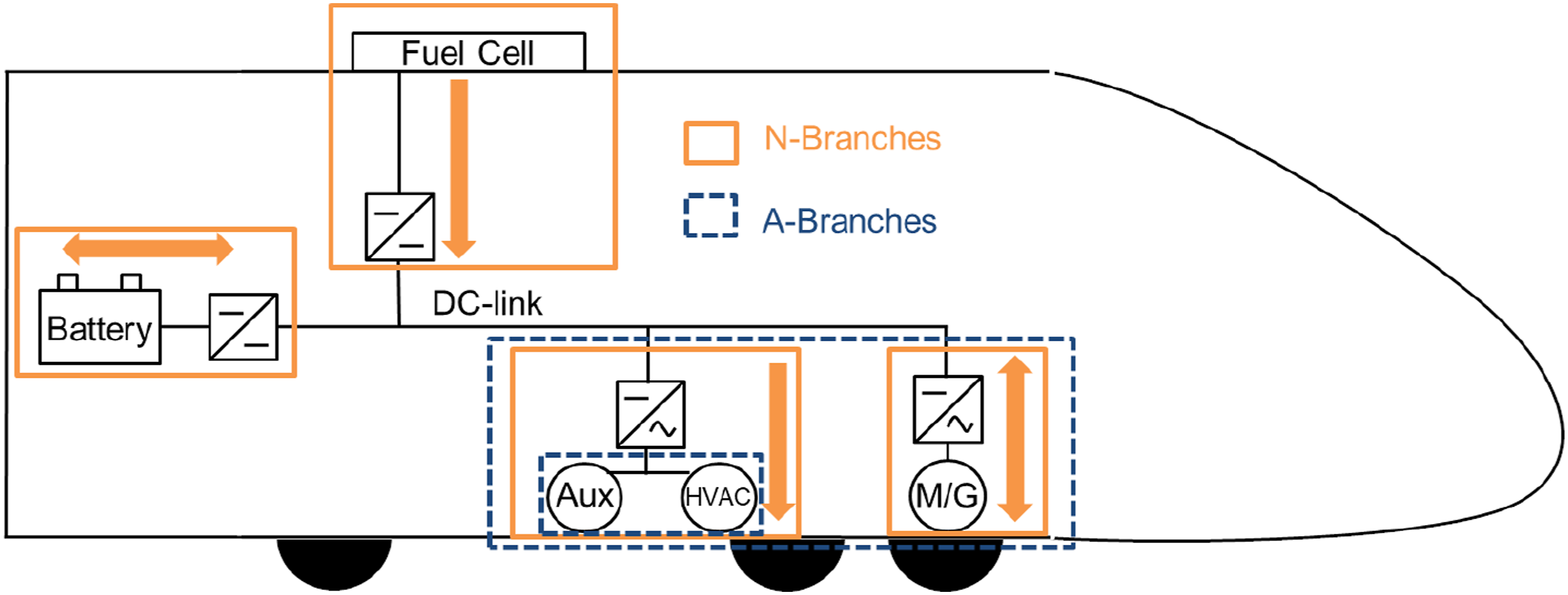
Through combinations of these two branch types, the construction of the symbolic representation of objective functions and constraints can be fully automated. After automatically generating symbolic derivative matrices in form of the Jacobian and Hessian for faster optimization, all symbolic representations are then transformed into MATLAB function handles. This eliminates all human effort required to manually calculate and define them.

Example: Powertrain with Bi-Modal operation

To demonstrate the capabilities of the new implementation, a complex powertrain architecture was chosen for optimization. Bi-mode trains as developed for example within the FCH2Rail EU-project ⁸ pose a particular challenge in modeling and optimization due to the combination of three power sources, that is hydrogen fuel cell, a battery and overhead power supply via pantograph (see Figure 2). For these trains, optimization is of high interest as an efficient energy management strategy is complex to determine and thus energy consumption may be unnecessarily high with an unsuitable control.

Figure 2.

Schematics of bi-mode train architecture, consisting of fuel cell, battery and overhead line power sources.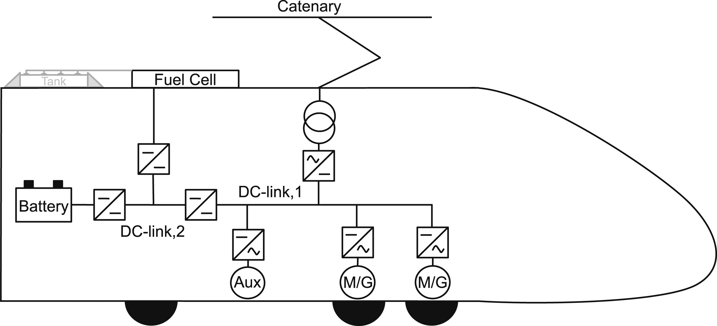

In order to optimize the energy consumption of a bi-mode train, there is a distinction from the objective functions used for Battery Electric Multiple Units (BEMUs) or Fuel Cell Electric Multiple Units (FCEMUs), as power drawn from two external sources has to be reduced in parallel. Thus, the objective function has to account for both catenary (P_cat) and fuel cell consumption (P_FC,chem):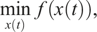

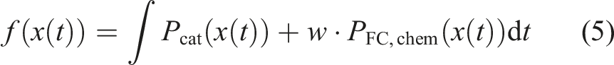
$\underset{x\left(t\right)}{\min }f\left(x\left(t\right)\right),$

where

$f\left(x\left(t\right)\right)=\int P_{\text{cat}}\left(x\left(t\right)\right)+w\cdot P_{\text{FC},\text{chem}}\left(x\left(t\right)\right)\mathrm{d}t$

(5)

All power drawn over the system boundary is summed up, which in the case of the overhead line is electrical energy and in case of the fuel cell chemical energy, both in kWh, with w being a weighting factor between the two energy sources. A w > 1 indicates that that the hydrogen energy is ”more valuable” as it is limited in the onboard storage and leads to a more flexible operation, since higher range is enabled when utilizing more power from the overhead line. Because the optimization does not consider detailed costs for now, a w of two was chosen. The energy drawn from the battery is optimized implicitly, because a charge-sustaining operation is enforced through boundary conditions. This means the initial state of charge has to be met in the end of the simulation, forcing the battery to be recharged by either power source which are part of the sum in the objective function.

Furthermore, the power balance has to be fundamentally adapted in order to represent the power distribution on the DC-link according to the more complex structure of the bi-mode power train. In comparison to previous implementations,^5,6 the blending factors θ and ϵ have been removed and replaced by a more efficient power balance constraint on the DC-link, considering all consumers P_DC−link,i on the DC-link.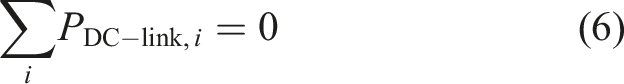

${\displaystyle \sum }_i{P}_{\text{DC}-\text{link},i}=0$

(6)

For the bi-mode train, the equation has to be slightly adapted due to the existence of two separate DC-links: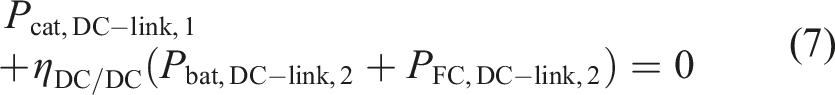

$\begin{array}{l}{P}_{\text{cat},\text{DC}-\text{link},1}\\ +{\eta }_{\text{DC}/\text{DC}}\left(P_{\text{bat},\text{DC}-\text{link},2}+P_{\text{FC},\text{DC}-\text{link},2}\right)=0\end{array}$

(7)

Here η is the functional representation of the power transformation of the DC/DC-converter between the two links. The new implementation allows for straight-forward adaptation of the power balance constraint by defining the branches correctly (see previous section).

Use and test case parameters

For all analyses, a generic regional vehicle is used as a basis. To analyze the overall performance of 2D efficiency model on SEnSOR, different train types were considered:

• a generic Electric Multiple Unit (EMU) with catenary power supply,

• a Battery Electric Multiple Unit (BEMU) with catenary and battery as power sources,

• and a Fuel Cell Electric Multiple Unit (FCEMU) with a fuel cell and a battery.

Each vehicle type has slightly different component sizes with regards to battery and fuel cell, but the train hull is the same. Key parameters of the vehicles are given in Table 1.

Table 1.

Vehicle and track parameters.

Characteristic	Value
Train
Length	55 m
Static mass	124 t
Rotating mass	6 t
Nominal axle load	15.5 t
Max. Speed	140 km/h
Max. de-/acceleration	1 m/s2
Max. Power for traction and recuperation	1 MW
Auxialiary loads	50 kW
Davis coefficients A,	2 kN
B,	5 N/(km/h)
C	0.2 N/(km/h) 2
Max. Power fuel cell	240 kW
	(Bi-mode and FCEMU)
Energy content battery	177 kWh (bi-mode)
	310 kWh (FCEMU)
	354 kWh (BEMU)
Route	Test track	Use case: Plattling - Bayrisch Eisentsein
Length	20 km	143.3 km
Journey time with stops	26 min 10 s	150 min
Number of stations	5	21
Net elevation gain (one way)	5 m	400 m

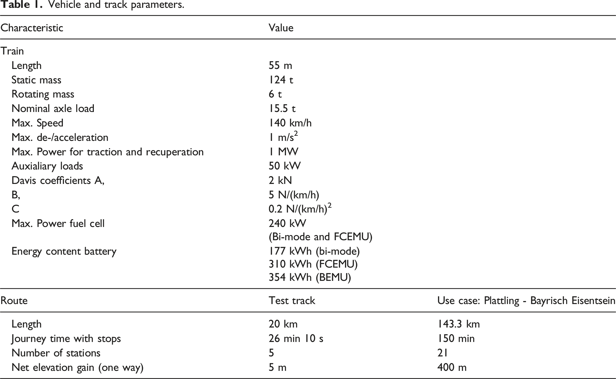
For the performance of the efficiency representation, a short 20 km test route with five stops as developed in 5 is used, to generate multiple results quickly. In this case relative comparison is of higher interest than absolute consumption values. The main optimization use case with the bi-mode train is then run on a hilly regional track between Plattling - Bayrisch Eisentsein - Plattling in Germany. Except for the assumption of additional electrification, this route is adopted from Kühlkamp. ⁶ Additional electrification was placed in the form of charging points at the junctions in Gotteszell (33 km) and Zwiesel (58 km), as well as a 3 km long section at the turning point in Bayerisch Eisenstein. The key characterists of this long track are given in Table 1 as well.

Results and discussion

Modeling and approximation error estimates

In the beginning of the paper, we postulated that the 1D approximation assuming a uniform behavior across all speed levels creates a significant model error and thus a more detailed representation in for of the 2D approximation is required. We verify this hypothesis using validated, generic component model data from the EU project FINE-1 ¹² (relevant components: motor and traction inverter). The upper part of Table 2 summarizes the error of the 1D functions in approximating the original 2D data points. The quality of fit of the analytic functions to the given data points were estimated using set of metrics:

• Root mean square error (Δ _RSME ) between the values at the given discrete 2D data points and the function evaluated at these points

• L1 error (Δ_L1) as normalized integrated difference between the constructed function and multi-linear interpolated function over whole 2D domain

Table 2.

Upper part: Approximation errors of the 1D power loss function when compared to the original 2D data points. Lower part: Errors of the 2D section-wise linear Chua functions in approximating the 2D data points and the contribution of error arising due to the smoothing procedure.

		Motor	Traction inverter
1D approximation error	Δ RSME (kWh)	0.063	0.02
	ΔL1 (%)	4.702	1.302
2D error estimates	Δ RSME (kWh)	0.009	0.002
	Before smoothing ΔL1 (%)	2.75 ⋅10−12	2.29 ⋅10−13
	After smoothing ΔL1 (%)	0.005	0.0004

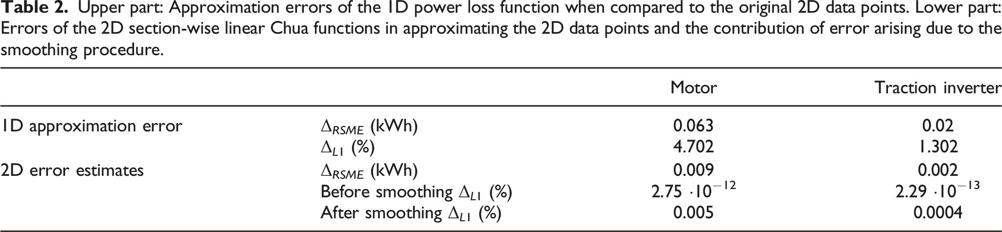
A more detailed definition of these metrics can be found in the Supplementary Material provided. One can see that the averaging effect of the efficiency introduce significant errors of almost 5% in the L1 error over the whole domain.

As expected, the errors of the 2D model are well below these numbers, as shown in the lower of Table 2. The modeling error in the first line indicates the approximation error of the 2D functions in fitting the 2D data points. Here, the 2D section-wise Chua functions reaches a similar quality of fit than it was possible with the previous 1D model. This highlights the power of the Chua functional representation in approximating given data points. With the L1 error, one can see that the major part of the error stems from smoothing. However, even after smoothing, the error between MATLAB’s non-smooth interpolated functions and the constructed smoothed section-wise Chua functions are lower than 0.01%. This is because the smoothing procedure only introduces errors very close to the sharp corners. Figure 3 shows the effect of smoothing procedure at non-smooth regions of a section-wise linear Chua function. Despite introducing errors at non-smooth region, it captures the overall structure of the data very well.

Figure 3.

The smoothed 2D section-wise linear Chua function fitted onto 2D power loss data of induction motor. The upper right hand corner shows the zoomed-in part of the smoothed function at a location that has sharp step change (marked region). This same location is shown without smoothing in the lower left corner.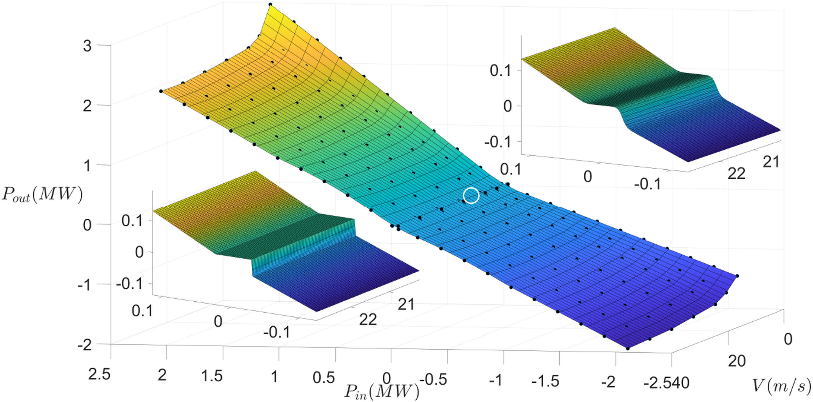

Effect of 2D efficiency model implementation on optimization results

In order to fully understand how significant the model errors are to the optimization, the effect of the efficiency models on SEnSOR results needs to be estimated. This was done by running simulations on the 20 km test route. The results of the optimization runs with 1D and 2D efficiency models are summarized in Table 3 for multiple powertrain architectures.

Table 3.

Energy consumption per km for different train types for 1D and 2D efficiency model, as well as the calculation difference caused by the application of the different models.

	1D model	2D model	Difference in %
EMU (kWh/km)	5.096	4.871	−4.62
BEMU (kWh/km)	5.600	5.249	−6.69
FCEMU (kg/km)	0.3058	0.2854	−7.15

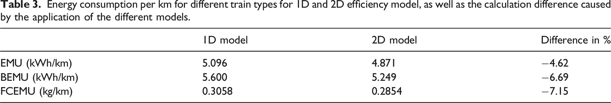
The difference in the optimization result indicates various inaccuracies caused by the simplification of using a 1D model. The analysis in the previous section showed that the 2D model results are more accurate with regard to the specified component efficiencies. The model error of the 1D model thus causes two issues in the optimization, which are of main interest: Non-optimality of the solution as a result of the simplification, and under-/overestimation of the total energy consumption even in case of optimal controls.

Detailed comparison of the solution variables shows that both issues are present: The 1D solution variables yield a non-optimal result if plugged into the 2D efficiency calculation and the 1D model overestimates the energy consumption, when applied on the 2D solution variables. The overall difference including both of these inaccuracies shows higher energy consumption for all train types when using the simplified 1D efficiency model. The difference increases from just below 5% for the EMU to over 7% for the FCEMU, thus with complexity of the powertrain architecture. The differences between the train types may be due to the fact that in BEMU and FCEMU there is additional power transfers within the train back and forth from the onboard energy storage. Due to the additional power losses, inaccuracies in the model are propagated and multiplied. With increasing complexity (e.g. number of components), this issue is amplified. Therefore, the new implementation shows greater benefit in BEMU and FCEMU than in EMU.

One of the disadvantages of shifting to a 2D efficiency model is an increase in the optimization time. Table 4 shows the summary of total optimization time required for each train type and for both the efficiency models. All computations were carried out serially on a Windows 64 bit system - Intel 5th Generation eight-core processor @ 2.40 GHz, 8 GB RAM. One can see that the time taken to optimize increases for all train architectures, above 50% for EMU and minimum of around 34% for FCEMU. With significant differences in the optimization results, indicating higher accuracy of the 2D, one has to decide depending on the application if the advanced 2D model shall be applied, as a trade-off between computational time and accuracy. For offline optimization and generation of benchmark results, the suggestion is to utilize 2D efficiency models, as computational performance is not of criticality. Currently, the initial guess for the battery and fuel cell variables are obtained using simplified calculations. It is expected that part of the computational time can be compensated by providing an improved initial guess which was out of scope for this study. A better initial solution leads to faster convergence of IPOPT to the optimal solution.

Table 4.

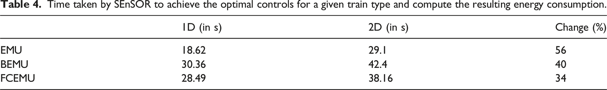
Time taken by SEnSOR to achieve the optimal controls for a given train type and compute the resulting energy consumption.

	1D (in s)	2D (in s)	Change (%)
EMU	18.62	29.1	56
BEMU	30.36	42.4	40
FCEMU	28.49	38.16	34

Results of the modular, flexible powertrain implementation: Bi-Mode train

As described in the implementation section, the bi-mode powertrain is chosen to demonstrate the capabilities of the new implementation. This, in particular, was done by running the simulation on a real route between the Plattling - Bayrisch Eisentsein - Plattling in Germany. We were able to implement the complex powertrain architecture in a straight-forward way and gain converging optimization results. With a computational time of around 16 min, the model results in an energy demand of roughly 315 kWh at the catenary and 10.8 kg hydrogen for this specific scenario and the combination of the chosen track and vehicle.

Figure 4 shows the results of the optimization. In the upper graphic, the speed and power control setting (throttle demand) are shown. The lower one illustrates the power split on the main DC-link. Both are for a specific uphill segment of the track. During the acceleration and cruising phase (approx. between minute 17 and 24), the fuel cell is running around maximum power to provide the base load, while the battery follows the remaining power request. Where possible, the fuel cell also slightly reduces its power to operate in a more efficient operating point. In the coasting section without traction demand (minute 24 to 26), the auxiliaries are covered directly by the fuel cell and the batteries are not used. Then, during braking and standstill phase (minute 26 to 30), which is partly under catenary, the fuel cell operates in idle mode. First, the battery stores the recuperative energy from the electro-dynamic brakes (just after minute 26). Afterwards, it is recharged at maximum power by the overhead line, which also supplies the auxiliaries required in standstill. Finally, the catenary supports the acceleration process of the next section, before the behavior repeats again in the non-electrified part of the section. The power split fulfills the given physical constraints and follows a logical behavior, thus giving the expected results.

Figure 4.

Results of bi-mode train optimization: power demand at the DC-link and split between the different power sources in MW for a specific section between minute 16 and 34 of the track.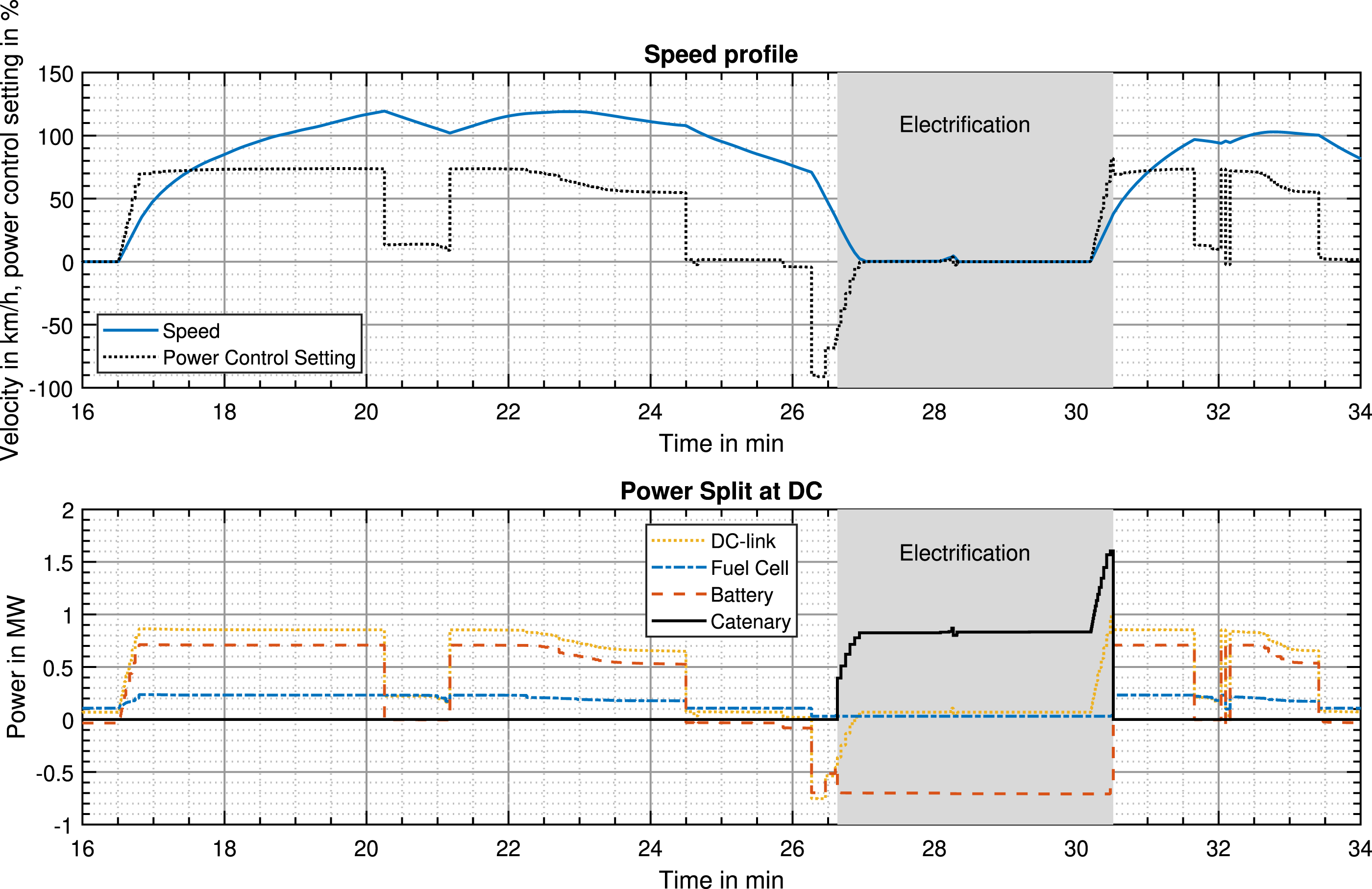

Figure 5 shows the cumulative energy demand over time. For the battery, the energy fluctuates around zero due to recharging processes on the route, with a maximum discharge of around 100 kWh. The final value settles at 0 kWh, since charge-sustaining operation is enforced. Thus, the total energy consumption consists of electric power from the catenary and hydrogen energy. Naturally, the energy drawn from catenary only grows in the electrified sections of the track and otherwise stays constant, while the hydrogen consumed by the fuel cell has a steady increase. Both reach final values of between 300 and 400 kWh, with slightly higher value for hydrogen.

Figure 5.

Energy consumption profile over the course of the complete track in kWh for each power source of the bi-mode train.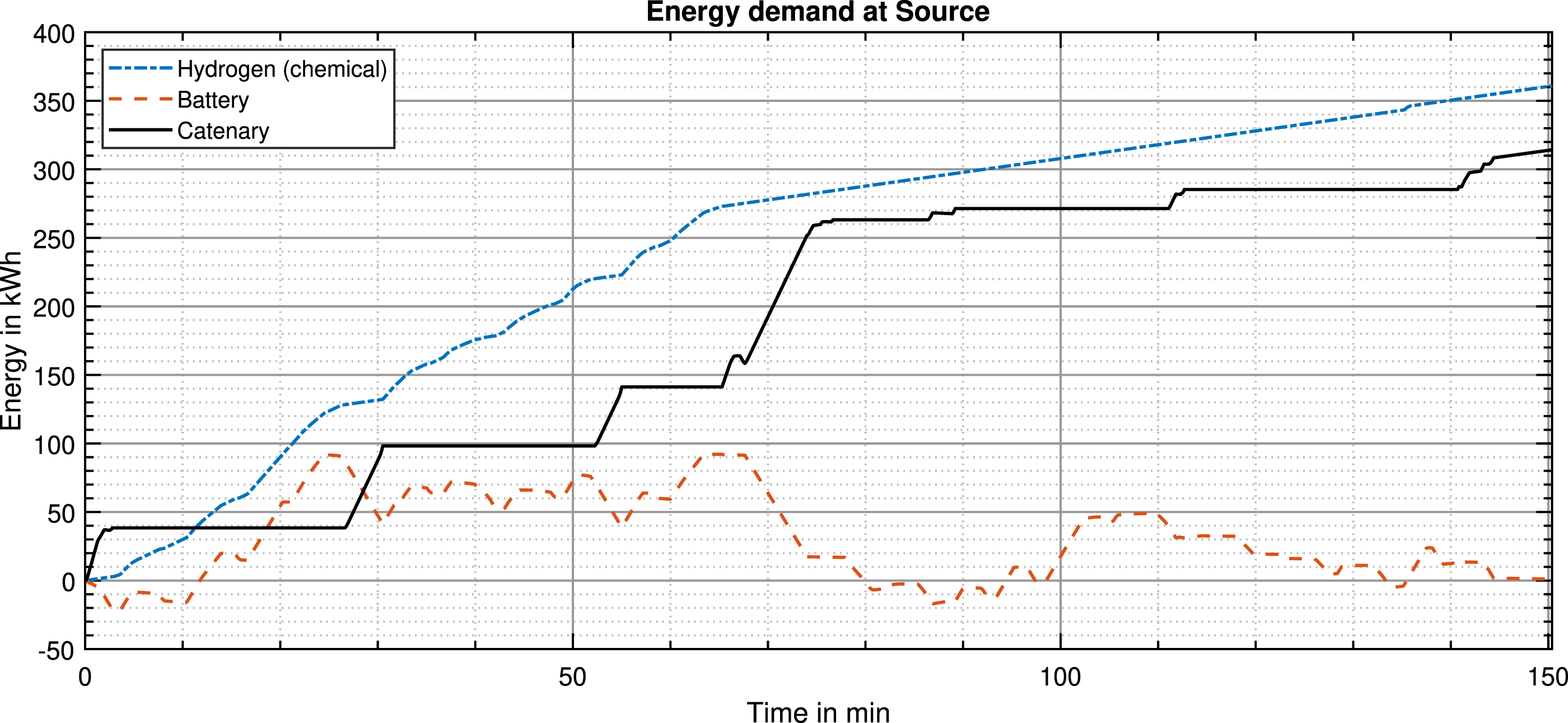

The total runtime remains almost the same with the new modular implementation. This comparison does not include the amount of manual pre-processing and debugging time required that goes into changing the OCP formulation with each change in the powertrain architecture. Therefore, the benefits are not objectively quantifiable, but noticeable in terms of effort required to optimize a new powertrain architecture.

Conclusions and future scope

The use and test cases demonstrate that the main goals achieved and the research question could be answered positively: integrating high-complexity constraints to reduce model errors and enabling highly modular flexibility to represent any powertrain architecture in the DM optimization algorithm SEnSOR. The first goal was analyzed with the implementation of two dimensional efficiency maps. Chua’s functional representation is computationally efficient and accurate in terms of approximating given data points. The availability of an analytic representation allows to easily perform mathematical operations on the represented data. Furthermore, the representation can be made smooth without significant information loss of the given data points (less than 0.01%). Sufficient smoothness is usually favorable to guarantee optimality of solutions obtained using higher order optimization procedure. Hence, this makes it a suitable choice in modeling OCPs. An enduring limitation is assumption of section-wise linearity between the data points. This strong assumption about efficiency maps may introduce significant model errors if the data set is coarse. For future works, it would be interesting to explore further approximations such as B-splines to study the robustness of the solutions to such changes.

The overall effect of approximation of the original data points onto lower dimensional space on the quality of solution is clearly evident from the results. The results suggest that the 1D approach overestimates the overall energy consumption and also yiels non-optimal results, especially in BEMU and FCEMU trains, with differences between 4 and 7%. With almost 45% average increase in computational time, the computational performance of the 2D-approach is lower than for the 1D-approximation as expected in the hypothesis. However, the decrease in model error is sufficiently high to justify the change in the model. Based on the modeling goal, one could choose to either use the 1D-approach for a quickly converging estimation. For all train types but the EMU, if accuracy is of higher importance, it is suggested to use the more complex model.

The second overarching goal of a modular, flexible algorithm structure to be able to handle a wide range of powertrain architectures and application cases was demonstrated with the successful optimization of the speed profile and energy management for a bi-mode train. The power distribution between three sources was implemented in a straight-forward way into SEnSOR. The results show convergence of a real world railway route within 16 min, minimizing hydrogen and overhead line electricity consumption at the same time. The power split between all power sources follows a reasonable behavior, with the battery covering peak loads and utilizing regenerative braking energy, as well as the catenary continuously recharging the battery and primarily covering traction demand. The fuel cell is used to cover base load and otherwise hold steady in a high-efficiency operating point. For optimization of operation, energy from overhead line and hydrogen could also be weight differently, if one of the power sources is preferential, for example with a cost model.

We showed the potential of DM optimization algorithms in offline railway simulation to reduce energy demand. Highly complex powertrain architecture are integrated easily and optimized within reasonable computational time. Future activities will focus primarily on further improving computational performance and thus potential applicability into real-time train control to offer optimized driving advice and energy management on the train.

Supplemental Material

Supplemental Material - Optimization algorithm for minimizing railway energy consumption in hybrid powertrain architectures: A direct method approach using a novel two-dimensional efficiency map approximation

Supplemental Material for Optimization algorithm for minimizing railway energy consumption in hybrid powertrain architectures: A direct method approach using a novel two-dimensional efficiency map approximation by Rahul Radhakrishnan and Moritz Schenker in Part F: Journal of Rail and Rapid Transit