Sage Journals: Discover world-class research

Abstract

This work presents the main problems in the primary suspension of metro vehicles and a methodology to detect those using wayside systems. The primary suspension is usually based on rubber elements, which are space saving and have damping properties. However, rubber characteristics change with time, often in a different way in each element. Differences between elements can cause irregular transmission of loads to the wheels, and thus, a reduction or loss of guidance forces. The ageing of rubber can also lead to a general stiffening of the primary suspension, which increases the risk of derailment. This paper presents a wayside system that uses a few strain gauge bridges to detect those problems independently of the vehicle load and speed. Firstly, the system is developed by means of a multibody model. Secondly, a demonstrator is installed in an operating metro exploitation. Finally, the accuracy of the predictions is proven by testing some of the elements in the laboratory.

Keywords

Railway primary suspension rubber elements condition monitoring

Introduction

The primary suspension of railway vehicles plays a key role in vehicle stability, curve behaviour and transmission of forces to the track. It is responsible for balancing the vertical loads transmitted through the wheel-rail contact, which prevents wheel unloading and improves wheelset guidance. A balanced load distribution also helps maintain the track in good condition. Moreover, the primary suspension filters dynamic forces and accelerations caused by track irregularities.

To achieve the above-mentioned functionalities, different primary suspension configurations have been used over time, most of them based on rubber elements. Compared to other elements, rubber elements tend to require less space and have damping properties as well as progressive stiffness characteristics. These properties enable rubber elements to satisfactorily meet the requirements of the increasingly demanding railway industry, favouring an increase in their use in all types of railway vehicles.¹

However, the use of rubber elements has some drawbacks that cause difficulties in the design and maintenance of railway suspensions based on these elements. The main problematic characteristics are listed below.

• Nonlinear characteristics: the relationship between stress and strain is not linear. Tension, compression, shear, torsion or buckling tests generate different load-deflection curves, but in all cases the ratio of the resulting stress to the applied strain is non-linear.²

• Amplitude and frequency dependence: the Fletcher-Gent effect or Payne effect^3,4 states that the deformation amplitude influences the dynamic stiffness of the rubber components. The Mullins effect⁵ describes the stiffness decrease experienced by rubber in the first few cycles when a cyclic load is applied to it. Experimental tests also show a rate-dependent behaviour, where the dynamic stiffness increases along with excitation frequency.

• Amplitude and excitation rates also influence other characteristic effects of rubber, such as stress relaxation, creep, recovery, or hysteresis, all studied by Gent.⁶ Elastic hysteresis is caused by internal friction of the material, which leads to energy dissipation and the aforementioned damping effect. Stress relaxation is the stress decrease observed at a constant strain, and it is related to hysteresis. Creep is the irrecoverable residual deformation that remains in a component after being subjected to a constant stress for a period of time, while recovery is the measure of the original dimension recovery of the rubber after strain release.

• Temperature is another variable influencing the dynamic behaviour of rubber.^7–11 It also conditions the deterioration of its properties.

• Variation with time and ageing: the deterioration of rubber depends on its working conditions but also on time. Moreover, it is already difficult from the manufacturing process to control the properties of rubber. Designed and achieved stiffness value differences of around 10% are considered acceptable.¹² Therefore, due to this time-changing nature of the material, the characteristics and ageing process of each rubber spring can vary.

There are two strategies in order to deal with the above-mentioned problems when modelling rubber components: the first one is developing special elements for Finite Element Model codes replicating the complicated micromechanics of rubber.^13–17 The second one is to develop lumped parameter models of rubber element components that simulate their macroscopic dynamic behaviour with very few parameters and low computational cost.^18–20

Nonetheless, the aforementioned rubber characteristics do not only influence the modelling process, but also the performance of rubber components in mechanical applications. In the case of railway rubber elements, the modification of characteristics with time is a key phenomenon that determines the maintenance operations: on the one hand, a general excessive stiffening of the elements reduces the capability of the suspension to absorb the trajectory variations and increases the risk of derailment. On the other hand, an irregular stiffening or variations in the creep leads to an irregular transmission of forces and a consequent damage to the rail, apart from increasing the risk of unloading of some wheels.

Due to that, it is necessary to perform maintenance operation in order to assure that the characteristics of the elements are within certain margins. In the cases where the stiffness of the elements exceeds limit values, the elements must be replaced. On the contrary, when the problem is related to height differences between elements (creep), the resulting imbalances can be corrected by introducing shims. These components are metal discs with given thickness values that allow the compensation of the differences between the elements.

It is worth pointing out that the measurement of the rubber elements’ stiffness once they are mounted is not easy. In most cases, it entails the separation of the bogie from the carbody and subsequently primary suspension dismantling. This operation is time consuming and expensive. Instead, elements are usually replaced at fixed time periods without considering the actual condition. In more frequent maintenance stops, the height of the elements is checked and in case there are height differences, shims are introduced.

A methodology that allows the condition of primary suspension elements to be checked continuously would help not only to maximise the life of elements, but also to optimise the scheduling of maintenance stops, and thus, to save time and reduce costs while maintaining or increasing safety standards. This paper presents the development of a low-cost wayside monitoring system that allows the study of the evolution of the primary suspensions’ condition and the detection of their defects while the vehicles are running in service. The system uses the signals from strain gauge bridges installed on the rail in both straight track and curve transition; these devices measure the elastic deformation caused by the load transmitted in the wheel-rail contact, and from there the contact force can be inferred. Based on each wheel’s contact force information, the following section presents a methodology to assess the condition of the primary suspension of all the vehicles passing over that track section.

In the “Primary suspension condition monitoring system” section, the technical viability of the system is proved using a multibody model. Then, results obtained in a demonstrator of the system are presented in “Primary suspension monitoring system results.” Finally, in the section “Validation of wayside results by detailed experimental tests,” the accuracy of the system predictions is confirmed with the results from laboratory tests.

Methodology for assessing the assessment of primary suspension condition

Critical parameters

The objective of this section is to describe the methodology (measurements and signal analysis) required to characterize the status of a primary suspension system in operational conditions as determined in this research project. A multibody model of a railway vehicle was used to understand the influence of the different parameters in the signals and the way to relate them to the different deterioration phenomena. The model was developed and verified both in Sidive and Vampire.

In order to carry out the simulations, a 145 m long curve, with a radius of 200 m and a cant of 120 mm, will be used along the section. Before and after the curve, two 100 m long straight sections were included and two clothoid curves of 55 m used in the transitions between curved and straight track. Figure 1(a) shows schematically the track (in the upcoming graphs the vertical dashed lines represent the limit between the described different track sections). The analysis focuses on the vertical contact forces, which are variables that can be easily estimated using strain gauge bridges. The considered vehicle is a standard metro vehicle. Figure 1(b) shows the scheme of the coach and the indexes that will be used to refer to the different wheels.

Figure 1.

(a) Layout of simulation track, (b) Scheme of the vehicle used in the simulations and the abbreviations to refer to the wheels.

Figure 2(a) shows the vertical wheel-rail contact force of the different wheels in the leading bogie when the stiffness in all the suspensions is the nominal and there is no creep. In the straight section (0–100 m), the load distribution is uniform and the contact force is close to 55 kN in all the wheels. When the vehicle reaches the transition (100–155 m), since the curve goes to the right, at 60 km/h the load on the left front wheel (1L) increases due to the progressive cant increase in the left rail. At this phase, a completely rigid bogie would be supported on three wheels (1L, 2L and 2R) while the remaining 1R wheel would be completely unloaded. Thanks to the primary suspension elasticity, the front right wheel (1R) does not lose contact, although it is partly unloaded. When the transition ends and the part with constant radius and cant is reached (155–300 m), there is a load reduction in 1L and an increase of load in 1R, achieving a new force balance driven by the centrifugal force and the curve cant. In the exit transition (300–355 m), where the cant and curvature is reduced, the process is the opposite: the load in 1L diminishes and the 1R load increases until ending the transition, where the initial balance is recovered (355–450 m). As far as the rear wheels are concerned, the load variations are lower along the whole curve, although the initial impulse when the bogie enters the transition is still high.

Figure 2.

Vertical contact load variation of the front bogie wheels along a curve, with different primary suspension stiffness values: (a) All the wheels the same nominal stiffness, (b) Stiffness of the 1L wheel suspension 30% higher than the rest, c) 3 mm creep in the 1L wheel suspension.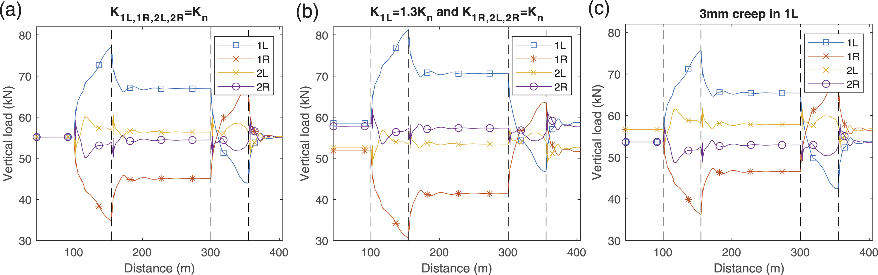

When there are differences in the stiffness characteristics of the elements in the same bogie, the distribution of loads on the wheels changes. An example is shown in Figure 2(b), which represents the vertical loads of the wheels of the leading bogie when the stiffness of the suspension in 1L is 30% higher than the rest. Looking at the load values in the straight, the stiffness increase in 1L causes the deformation of that wheel to be lower and, hence, it supports a higher part of the load. This unbalance makes the largest part of the rest of the load to fall on the wheel of the bogie furthest from the defective suspension wheel, the one diagonally opposite. Meanwhile, the load on the wheels of the other diagonal become lower. If the difference between elements comes from a creep problem, there is also a variation in the distribution of the loads. Figure 2(c) shows the load of each wheel in the bogie when there is a 3 mm creep in the 1L element. Contrary to what is observed in the case of Figure 2(b), the lower height of the element in 1L causes a higher ratio of the total load to fall on the wheels of the opposite diagonal, i.e. 1R and 2L. Also, it can be seen that the variation of vertical forces during the curve negotiation is different in the three situations (nominal, stiffness problem and creep problem).

The examples represented in the graphs b and c of Figure 2 show how a change in either the stiffness or the height (creep) of the suspension, leads to a different distribution of the loads in comparison to the nominal case shown in graph a. In a straight section, there is an increase in the loads of one diagonal and a decrease in the other diagonal. Therefore, the definition of a parameter that considers the loads of the diagonals in pairs can be a useful indicator: bogie-twist, $F_{1}$ , defined in equation (1).

F_{1} = \frac{(F_{1 R} + F_{2 L}) - (F_{1 L} + F_{2 R})}{F_{1 R} + F_{1 L} + F_{2 R} + F_{2 L}} \cdot 100

(1)

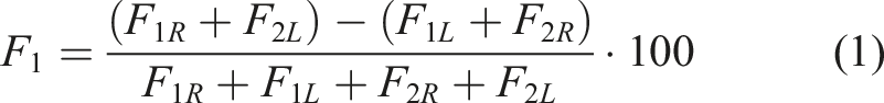
Figure 3 represents $F_{1}$ paramete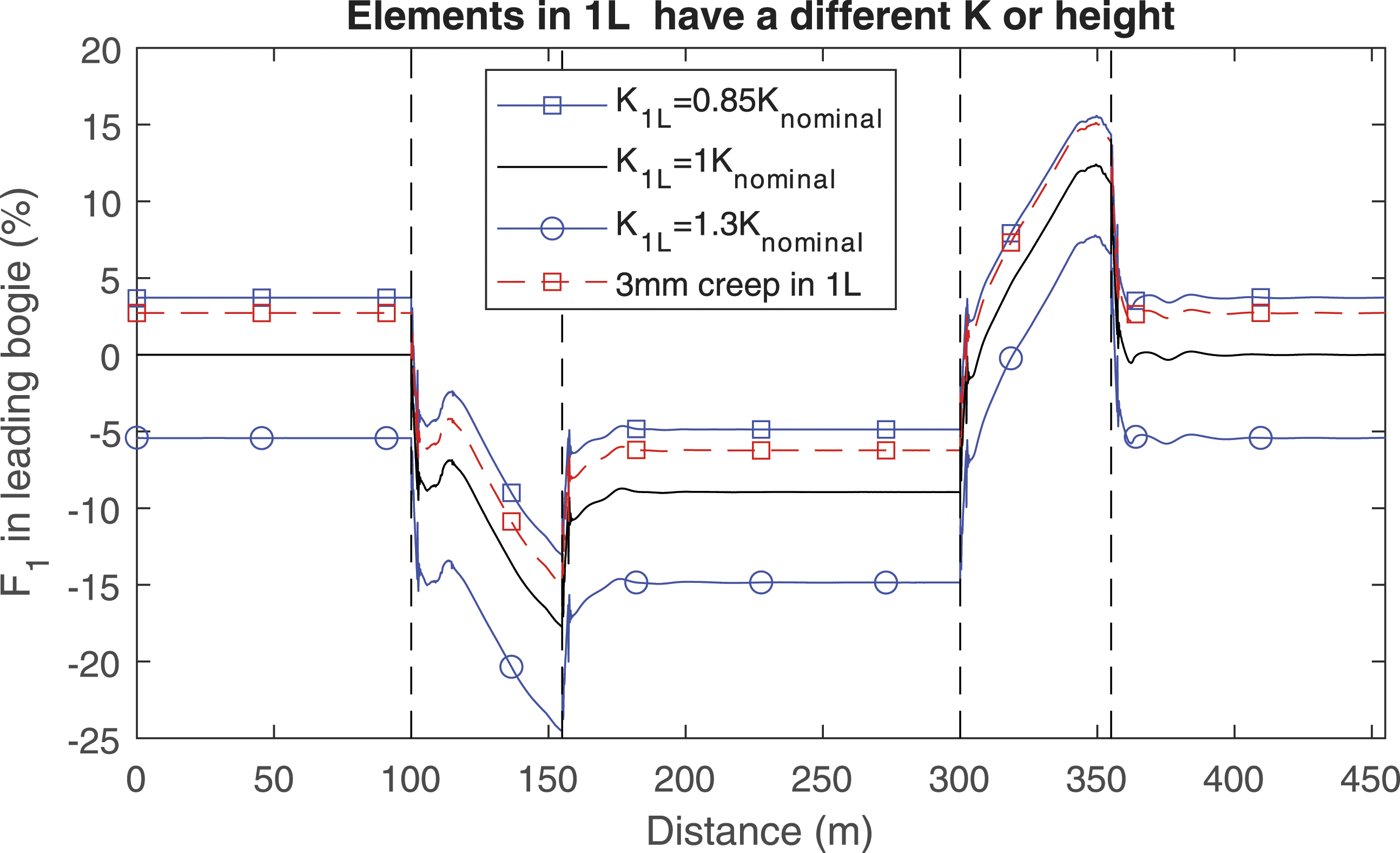rs in the previous simulations, which consider stiffness variations and creep in 1L. As it can be seen, the variation of the bogie twist in the straight, $F_{1}^{s}$ , allows the detection of the existence of a problem. However, it does not differentiate when the cause of a variation is a creep problem or a stiffness difference between elements; additionally, it does not vary when there are general stiffening problems either. Therefore, another parameter indicating variations in the stiffness of the primary suspension is required. This parameter is the bogie twist variation, $∆ F_{1}$ , which essentially is the bogie-twist subtracting the constant straight bogie-twist value, as shown in equation (2)

∆ F_{1} = F_{1} - F_{1}^{s}

(2)

Figure 3.

Bogie-twist, $F_{1}$ , when the stiffness or height in 1L varies with respect to the rest.

The value of 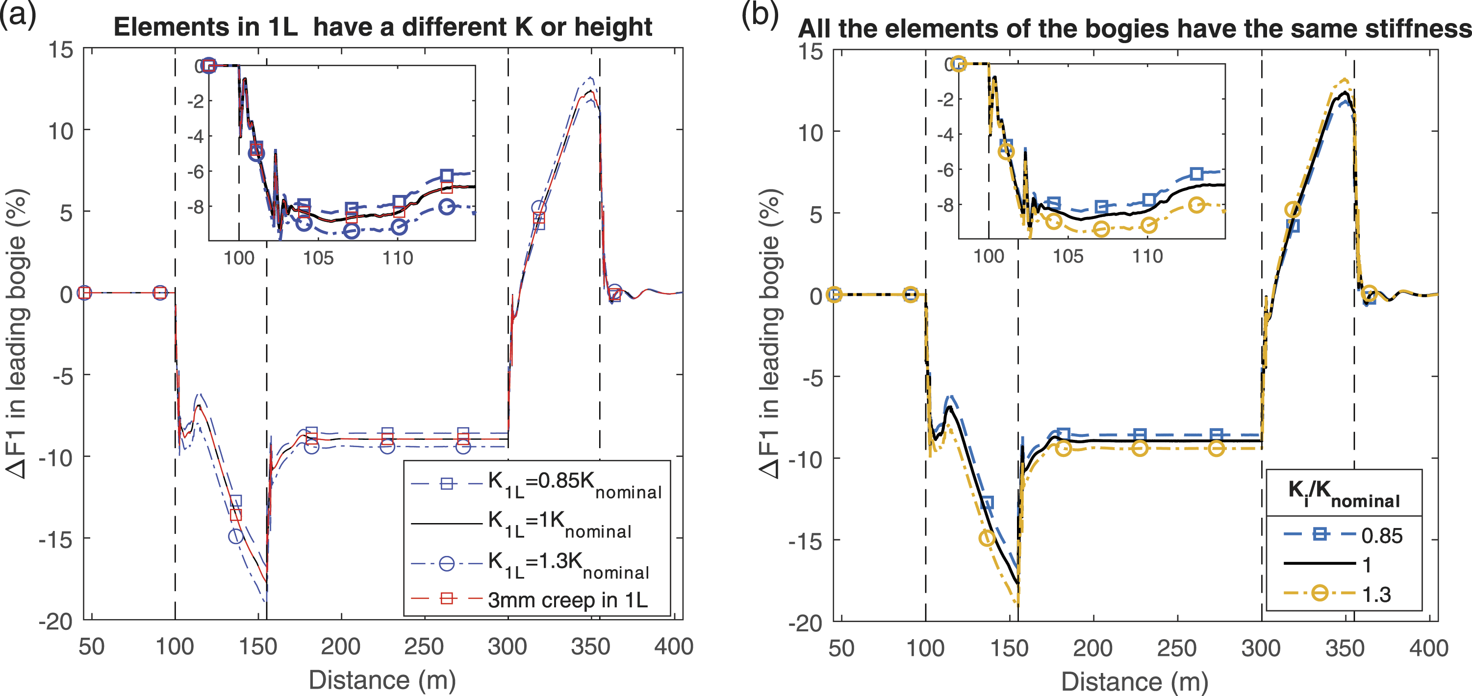$∆ F_{1}$ is always zero on straight track and it varies along the curve. It depends on the general stiffness of the primary suspension, and the creep has no influence on it. This is shown in Figure 4(a), where the value of $∆ F_{1}$ in the case with creep is exactly the same as in the nominal case, whereas for the cases where the stiffness in 1L is different, there is a small variation of $∆ F_{1}$ in the curve.

Figure 4.

$∆ F_{1}$ in the front bogie when: (a) 1L has a different stiffness or height than the rest of elements, (b) all the elements have the same stiffness.

When all the elements have changed their stiffness to the same extent and there is no creep, $F_{1}^{s}$ remains zero. However, Figure 4(b) shows how the value of $∆ F_{1}$ changes with respect to the case with nominal stiffness values along the curve.

In order to define the point where this value of $∆ F_{1}$ should be measured in the wayside system, it would be interesting to choose a position where the influence of the speed or the load would be minimum and the sensitivity to the different problems is maximum. The next section will analyse this issue.

Influence of speed and load

The circulation conditions of the vehicles vary between passages. Among these conditions, vehicle load and speed are especially relevant for the contact conditions between wheels and rail. However, there are some parts of the track where these variables do not influence the parameters $F_{1}$ and $∆ F_{1}$ .

In the straight part, as long as there are no wheel or rail irregularities, or variations in their conditions, vehicle speed does not considerably influence the distribution of the forces. In discretely supported tracks, the speed affects the parametric excitation, but the resulting variations in the bogie-twist parameter are not high enough to alter the estimation of the condition, as long as speed values remain within reasonable limits.

As for the influence of the load variations, as long as the distribution does not vary, the conclusion is the same and the bogie-twist parameter does not perceptively change. The reason is that in the formula of the bogie-twist parameter the subtraction of diagonal sums is normalized by the sum of all the loads.

In the curve, other factors, such as the inertia related to the lateral unbalanced acceleration, come into play. The speed and the load affect this centrifugal inertia, and the variations of these variables produce differences in the bogie-twist parameter. However, in the first part of the transition of the curve, the influence of the load and the speed are still negligible, as shown in the example of Figure 5. The bogie twist in the initial part of the transition (in the example from 100 m to 114 m) is mainly affected just by the stiffness of the primary suspension elements in the bogie and therefore, the measurement of the wayside system should be done there.

Figure 5.

Bogie-twist variation, 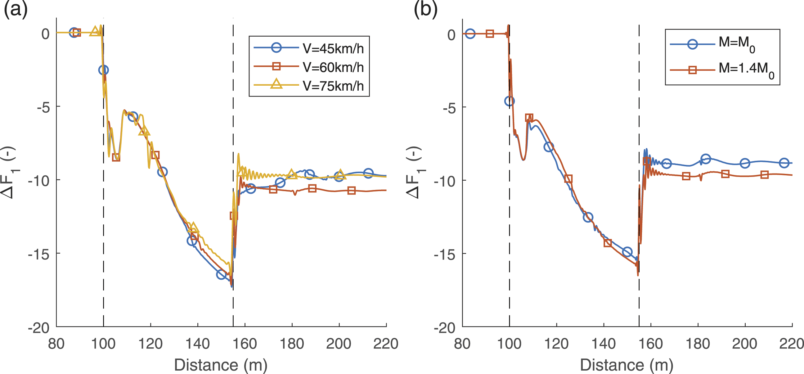$∆ F_{1}$ , for different values of: (a) speed, (b) load.

More precisely, the area of interest would be the part of the transition where all four wheels are already in the transition but the flange contact has not occurred yet, since at that point lateral forces would increase and the speed and the load would start to influence the $∆ F_{1}$ parame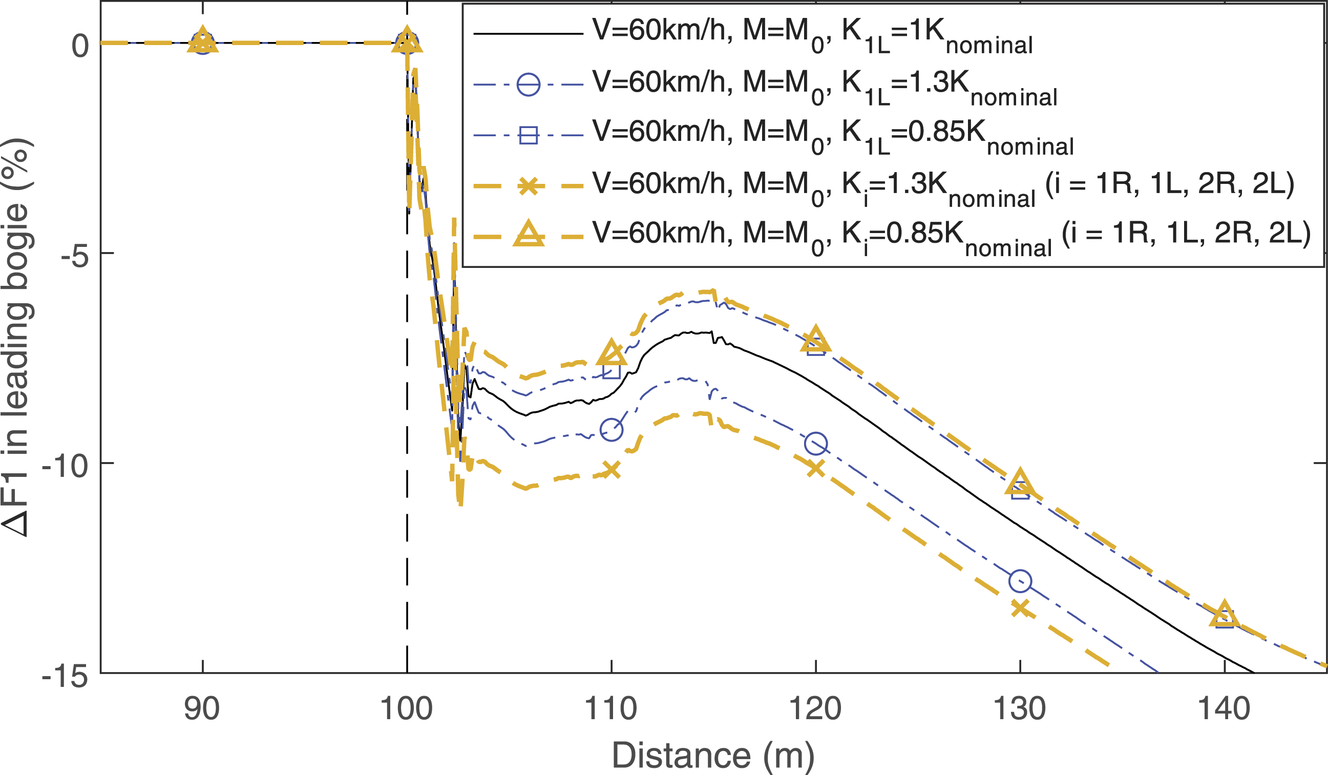ter. Figure 6 shows how the stiffness variation in one of the wheels (dash and dot style lines with circles and squares) or in all the wheels (dashed lines with crosses and triangles) generates a $∆ F_{1}$ variation in that zone where it is unaffected by the load or the speed.

Figure 6.

Detail of $∆ F_{1}$ in the start of the transition before the flange contact when one or all the elements present different stiffness values.

In the case of the curve with 55 m transitions, which is the curve where the field study is done, the area of interest from the start of the transition for the measurement of the 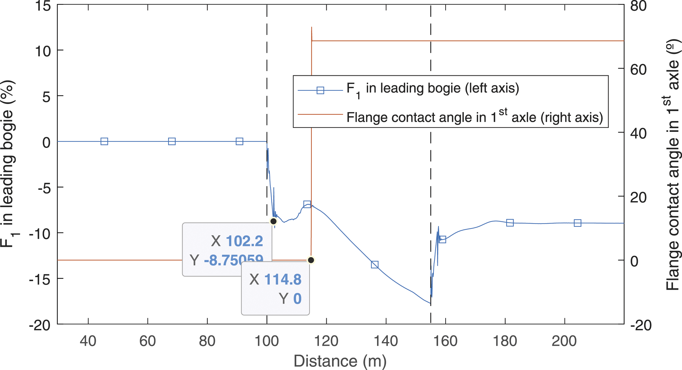$∆ F_{1}$ parameter is between 2.2 m, which is the wheelbase of the vehicle, and 14.8 m, which is the point where the flange contacts the rail. Figure 7 represents the bogie-twist as well as the flange angle in the transition; the flange angle of the 1st axle becomes different from zero when the flange contacts the rail.

Figure 7.

$F_{1}$ and flange contact angle of the first axle of the first bogie in the curve introduction transition.

Once the parameters that are sensitive to the defects in the primary suspension are defined, the next section will analyse how to determine the primary suspension condition.

Procedure to determine the condition of the suspension

The previous section has studied the influence of the most common defects in the primary suspension—creep, isolated stiffness variations and general stiffening—on the bogie-twist and bogie-twist variation parameters. It is shown that with the measurements of the bogie-twist parameter in the straight, $F_{1}^{s}$ , and the bogie-twist variation in one point between 2.2 m to 14.8 m of the transition, $∆ F_{1}$ , it is possible to detect and identify any of those defects.

When

F_{1}^{s}

differs from zero, it means there is an irregular distribution of the loads, that can be caused by the creep of some elements or differences in their stiffness values. In the case of the former, the value of

∆ F_{1}

is the same as in the nominal case, whilst in the latter, there is also a variation in

∆ F_{1}

. In both cases, the wheel with the defective element could be identified looking at the load distribution. Finally, a null value of

F_{1}^{s}

combined with a variation of

∆ F_{1}

indicates the existence of a general variation of the primary suspension stiffness. This problem identification process is summarised in Table 1.

Table 1.

Primary suspension defect identification criteria.

	$F_{1}^{s} \neq 0$	$∆ F_{1} \neq {∆ F_{1}}^{n o m i n a l}$
Creep of some elements	Yes	No
Isolated stiffness variations	Yes	Yes
General stiffening of the elements	No	Yes

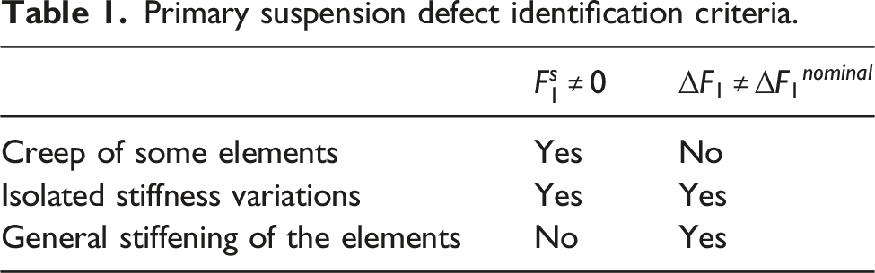
Once the problem has been identified, it is also possible to approximately quantify its extent. Figure 8(a) shows the relationship between the stiffness variation ratio and the resulting 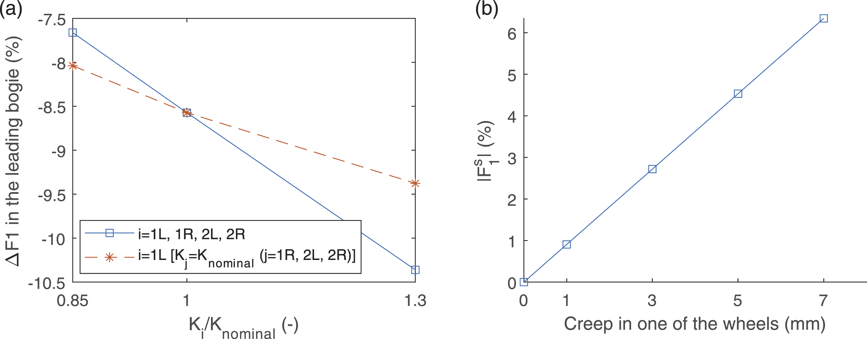$∆ F_{1}$ value measured 8 m from the transition start when there is a general stiffness variation (continuous line) or when the variation has occurred in a single element (dashed lines). Figure 8(b) estimates the absolute $F_{1}^{s}$ value for different creep values in one of the wheels of the bogie.

Figure 8.

(a) $∆ F_{1}$ in position 8 m of the transition for different stiffness values in 1L element or all the elements. (b) Absolute bogie-twist parameter value in the straight, $1 F_{1}^{s}$ 1 for different values of creep in a single wheel.

The next section studies how the parameters $F_{1}^{s}$ and $∆ F_{1}$ can be estimated from a few measurements in a real track.

Approximation of the bogie-twist parameter from discrete load values

In the simulations from the previous sections, the bogie-twist is calculated at every position along an extensive section of the track that includes a whole curve. However, it would be unfeasible to install strain gauges along such a long section of a real track. Instead, similar information can be obtained from measurements from sensors installed in specific locations of the track.

If it is assumed that the load distribution remains practically constant in a straight flat section of the track, the bogie-twist in a straight section, $F_{1}^{s}$ , can be calculated with one strain gauge bridge per rail. More strain gauges can be installed in equivalent positions of other spans to calculate the mean and reduce the statistical error. By installing these sensors in equivalent spots of the bays, differences in the measurement position receptance are avoided.

However, since the load distribution constantly varies in the transitions of the curves, using a single strain gauge bridge per rail does not work in the transition as well as in the straight. Therefore, in order to calculate the real bogie-twist parameter at a particular instant, the vertical loads of the four wheels of a bogie must be measured at the same time. This means that at least two strain-gauge bridges per rail, separated by the wheelbase distance, are recommendable.

However, in discretely supported tracks the tendency is to locate sensors in equivalent locations within the span when more than one measurement position is required. The reason is to make the installation process simpler and to ensure the same measurement conditions in the different sensors. Nonetheless, the wheelbase distance is not generally multiple of the bay length, so the two pairs of strain gauge bridges should be installed in different bays as close to the wheelbase distance as possible. In the case of the studied metro vehicles, the wheelbase is 2.2 m while the bay length is 1 m. Locating each pair of bridges in the centre of every other span, separated by 2 m, is the closest arrangement to approximate the wheelbase distance.

Another simpler approximation is to use a single pair of strain gauge bridges to measure the load on the four wheels of the bogie. In this approach, the measurement of the load on the second wheelset would be taken with a time delay equivalent to the time needed to travel the wheelbase distance, in this case, 2.2 m.

Figure 9 shows the simulated bogie-twist evolution in the beginning of the transition for the nominal case where all the elements have the nominal stiffness value, and the speed is of 60 km/h. In that case, the bogie-twist is obtained using the contact force values calculated in the four wheels of the bogie at the same instant. The two bridge-pair configuration, where the measurement of the second wheelset is taken with a time delay equivalent to the travelling time of 0.2 m, has almost no error with respect to the real calculation of the bogie-twist parameter. The error for the single bridge-pair approach, where the load of the second wheelset is calculated with a time delay equivalent to the travelling time of the wheelbase distance, is higher, but the configuration is not ruled out as it can provide values with lower accuracy albeit at a lower cost.

Figure 9.

Comparison of real bogie-twist parameter, 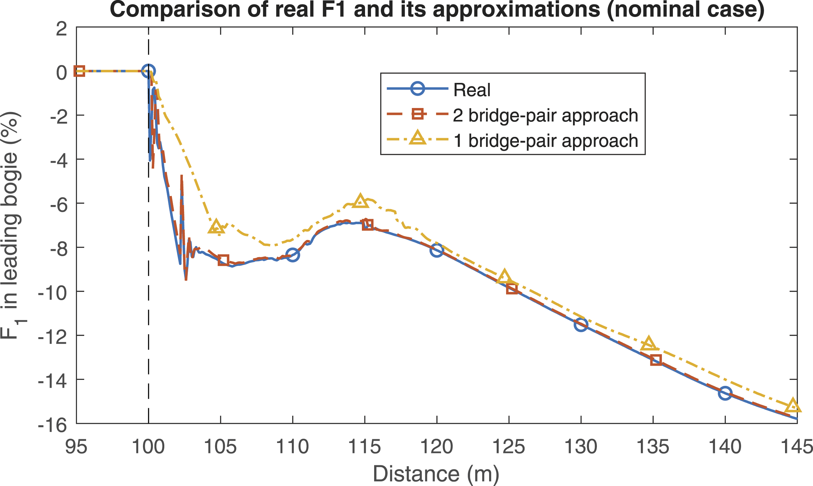$F_{1}$ , and its approximations, in the beginning of the transition for the 200 m radius and 120 mm cant curve.

In the present work the two bridge-pair approach is used for the installation of the sensors in the real track, as shown in the next section.

Primary suspension condition monitoring system

The results of the numerical analysis carried out in the previous sections shows the feasibility of a wayside system to assess the status of primary suspensions by measuring the vertical wheel/rail contact forces in two different situations: straight track and curve entrance. In this section, a prototype of a system based on these concepts is described.

Figure 10(a) shows the general scheme of the wayside system. The track where the system is installed includes a part with a layout which was the one used for the numerical simulations described above. In the straight section, three pairs of strain gauge bridges are installed in three adjacent spans, while in the beginning of the curve transition two bridge-pairs are located 2 m apart from one another, with a free span in-between. The use of three bridge-pairs in the straight allows the reduction of the deviations caused by the tread surface irregularities by calculating the mean value of the measured quantities. In the case of the transition section, the two bridge-pairs are located around 6 m and 8 m from the start of the transition, so that the calculated bogie-twist parameters correspond to the part where that parameter remains quite constant and is unaltered by the speed and the load.

Figure 10.

(a) Set up of wayside measurement system, (b) Configuration of the installed strain gauges.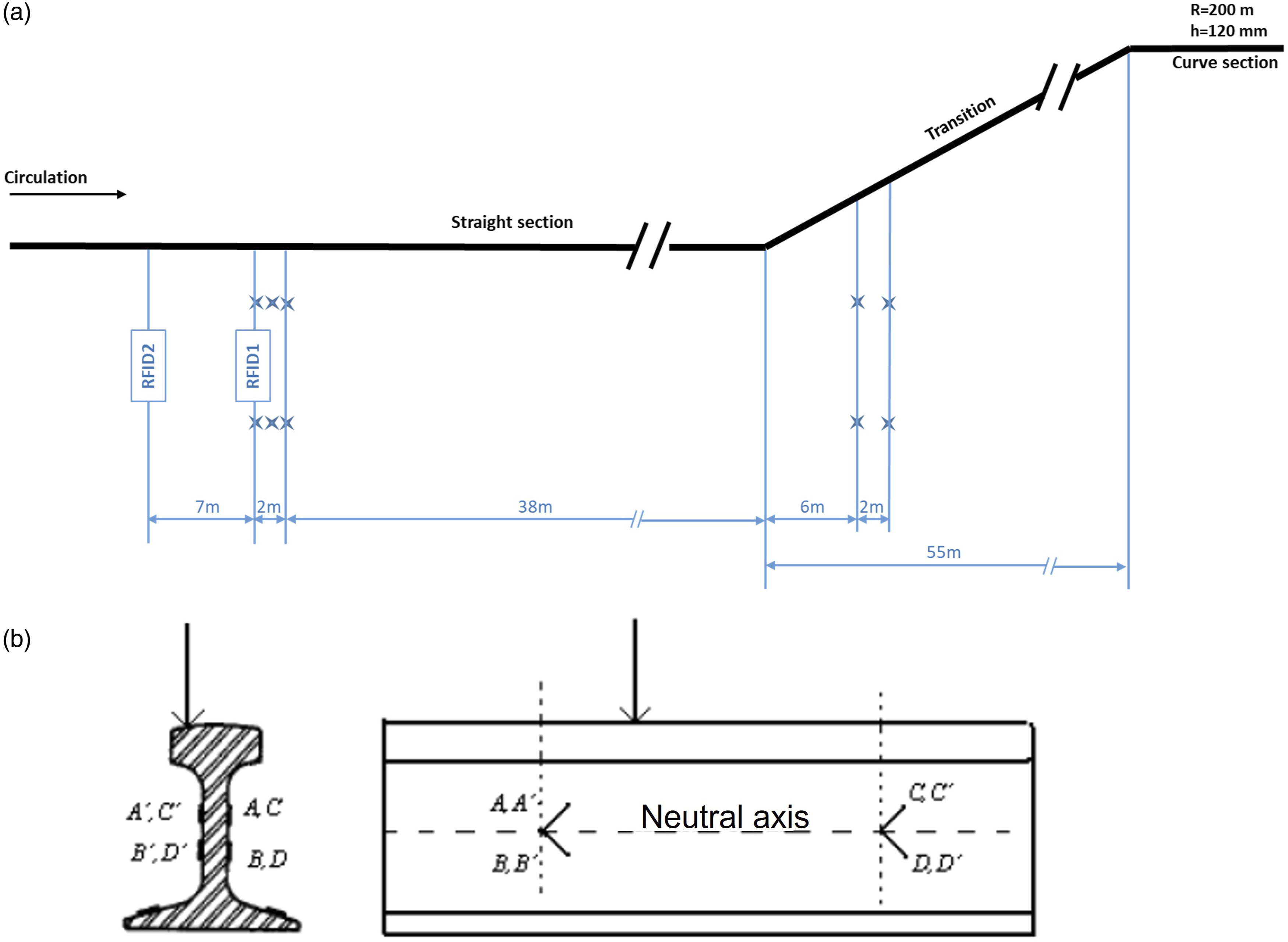

All strain gauges are installed at mid-span. In the transition, the two bridge-pair approximation approach explained in the previous section is applied. The measurements are obtained during the normal operation of the vehicles. In order to relate the measurements with the units, a RFID system is installed to automatically detect the unit passing over the system.

Figure 10(b) shows how the strain gauges are installed in pairs with a 45° angle with respect to the neutral axis. With this orientation, the shear strain of the rail causes a deformation and varies the electrical resistance of the strain gauges. The sensors have been calibrated in such a way that allows to infer the force that has caused that deformation from the resistance variation, and thus, calculate the wheel-rail contact force causing the rail’s shear stress. The standard deviation of the repeatability error in independent load measurements for a single bridge is proved to be around 2.5%. The use of three bridges allows a reduction of the error to 1.4%. The reliability can be further increased by considering consecutive measurements. For example, the use of 40 measurements reduces the standard deviation error up to 0.2%. This is why it is recommendable to analyse the evolution of the results considering several passages of the vehicle rather than looking at them individually.

The next section presents the results of the measurements obtained by the system over a period of 4 months for 340 different bogies, with 43,586 records in total (at least 57 passages per bogie).

Primary suspension monitoring system results

In order to check the accuracy of the measurements obtained with the wayside system, the results of the three different bridge-pairs located in the straight section are analysed here. Figure 11 shows the straight section load measurements as well as their mean, for the 1R wheel in one bogie of a specific unit (which is referred to as bogie A) in its different passages. The values obtained with the different gauge bridges for the different passages are always very similar. As the number of passengers changes in different passages, the load on each wheel also varies.

Figure 11.

(a) Set up of wayside measurement system, (b) Configuration of the installed strain gauges A.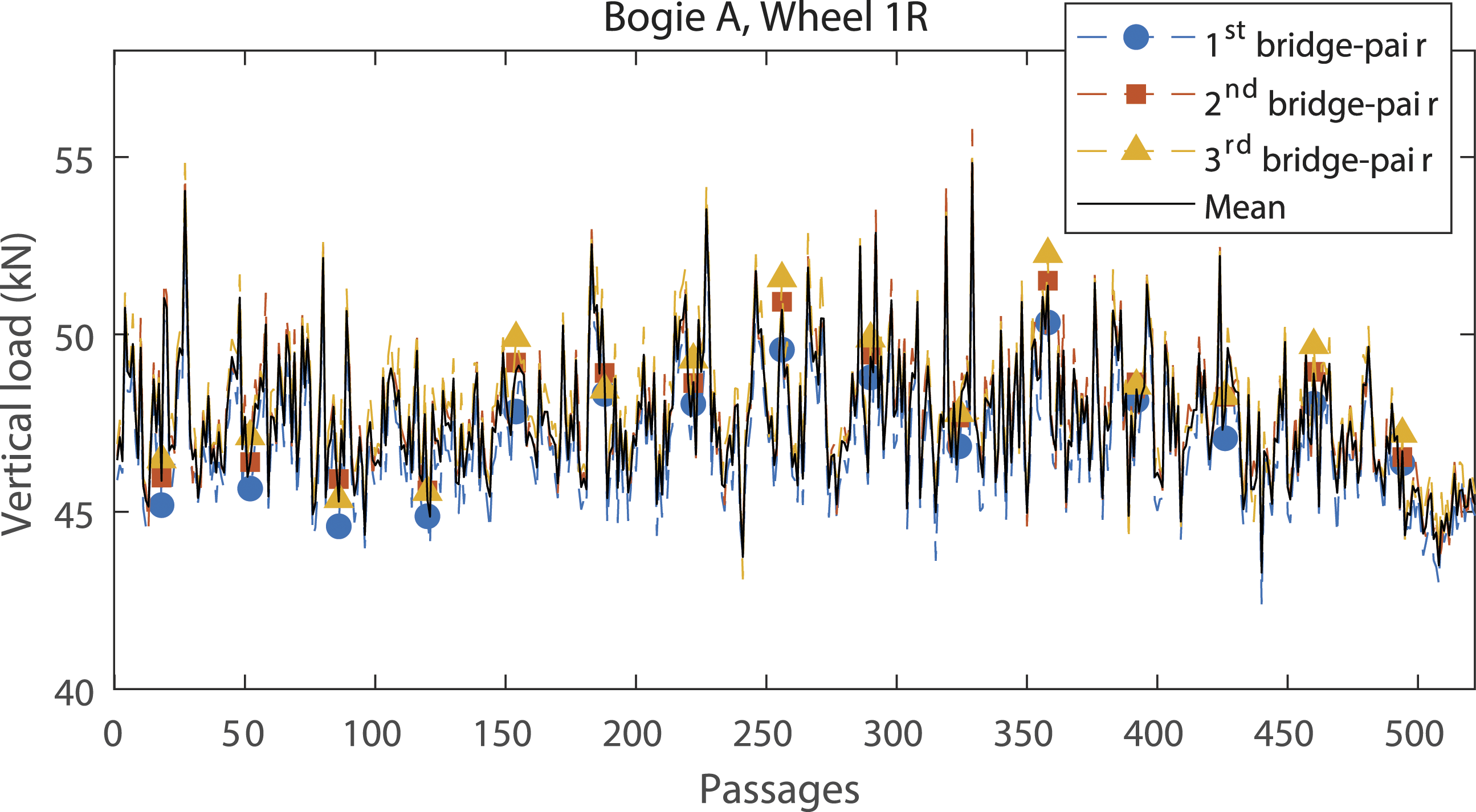

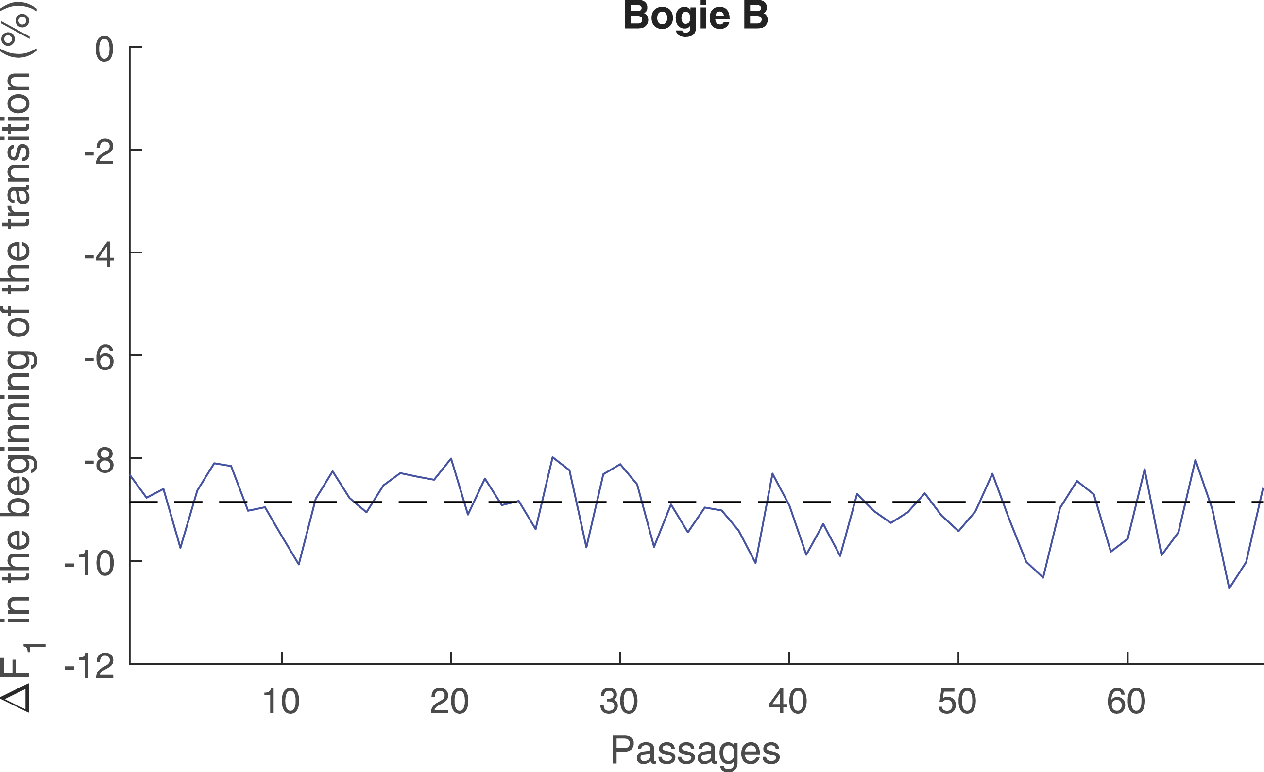
Figure 12 shows the bogie-twist parameter, $F_{1}^{s}$ , calculated using the mean of the load measurements (Equation (1)). As it can be seen, the obtained results are almost constant in all the different passages. In spite of the vehicle load varying, the obtained $F_{1}^{s}$ results are independent of it. Small differences between passages can be caused by many factors, such as little pitch and roll movements, track and wheel irregularities or wheel defects.

Figure 12.

Bogie-twist values measured in the straight part of the monitored metro track, 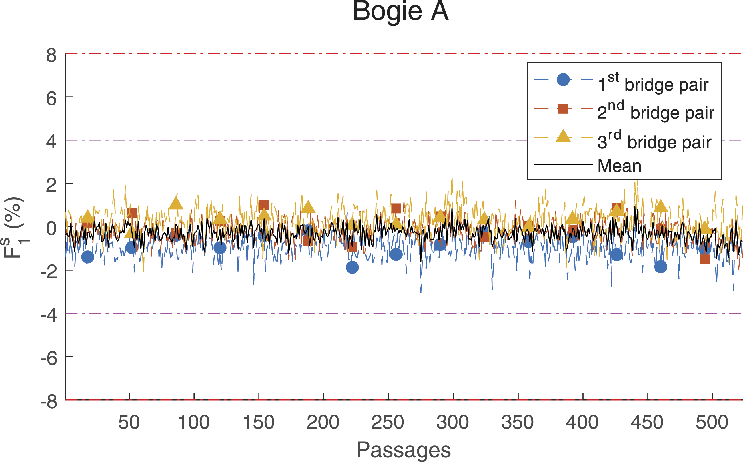$F_{1}^{s}$ , for the wheels in bogie A. The horizontal lines represent the limits in the current maintenance plan.

In the graph, the current limits in the maintenance plan are also included. The limits for $| F_{1}^{s} |$ should be set considering the maximum acceptable unloading values for the operating conditions of the exploitation. In this particular case, for $| F_{1}^{s} |$ values above 4% the vehicle can continue circulating, but a maintenance stop should be foreseen. For values above 8% the vehicle should undergo a maintenance procedure as fast as possible. As a consequence of this analysis it can be said that no maintenance stop must be foreseen for this unit.

In order to analyse the status of the chosen sample (340 different bogies have been considered), the distribution of the measured values is studied. Figure 13(a) shows the histogram of the bogie-twist values. As it can be seen, the distribution resembles a normal distribution, where the mean value is nearly zero and the standard deviation 1.76.

Figure 13.

Probability distribution of (a) the bogie-twist measured in the straight part of the monitored metro track, 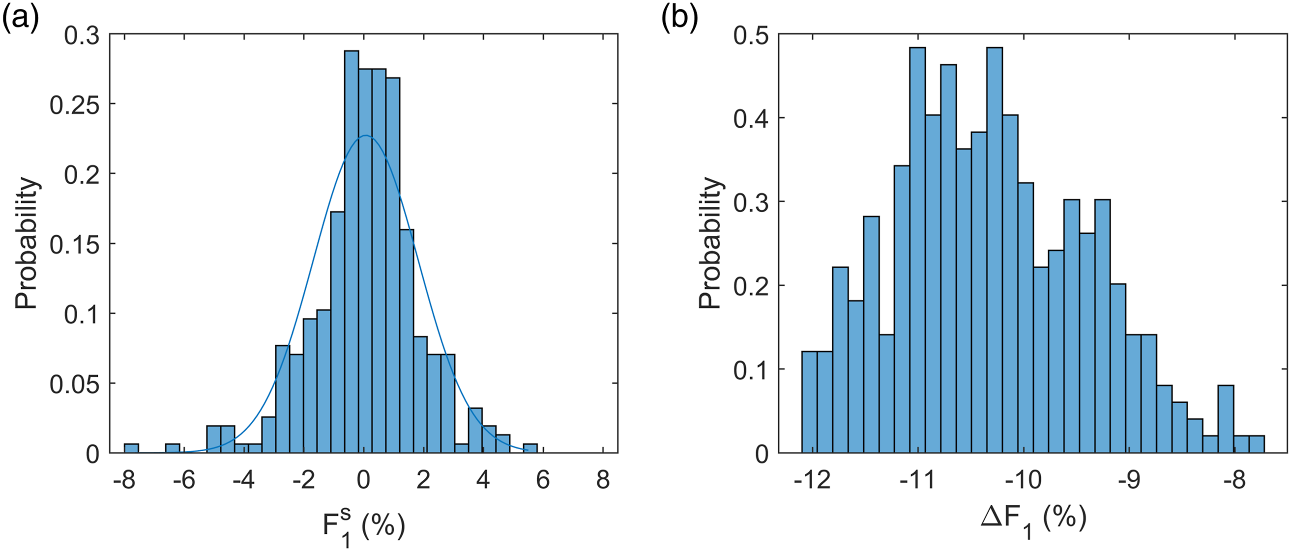$F_{1}^{s}$ , and (b) the bogie-twist variation, $∆ F_{1}$ , with all the measurements.

The results show that 96% of the studied bogies present $| F_{1}^{s} |$ values below 4%, meaning that their load distribution is uniform, and thus, the elements of their primary suspension are correctly compensated. This means that the height of the elements in all the wheels is similar (either because they do not present uneven creep or because the shims are correctly introduced) and there are no large differences in their stiffness. In 4.5% of the studied bogies $| F_{1}^{s} |$ is in the range 4–8 % and according to the limits in the exploitation a maintenance stop should be scheduled. Finally, there is no bogie exceeding the 8% bogie-twist limit. Therefore, it seems that the maintenance of the fleet is good and that the possible imbalances between elements have successfully been corrected.

Figure 13(b) shows the distribution of the calculated $∆ F_{1}$ values, where the mean is −10.31 and the standard deviation is around 0.9. The values are higher than those of the nominal case in the numerical analysis; looking at Figure 8(a), it seems that the general stiffness of the primary suspension in the operating vehicles is around 29% higher than the nominal value given in the plans. It might be because from the beginning the used elements are stiffer or because the stiffness has increased progressively with time.

Validation of wayside results by detailed experimental tests

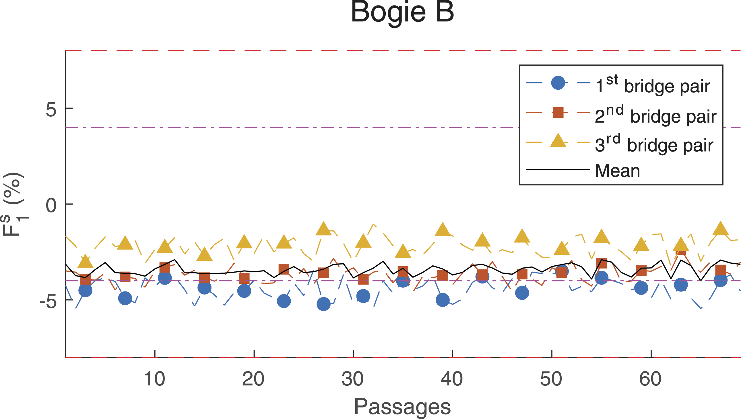
In order to check that the conclusions drawn with the wayside systems are sound, a detailed analysis of all the primary suspension elements of two bogies from different vehicles (bogie A and B) have been conducted to determine their stiffness and creep values. Both bogies underwent an overhaul where all the primary suspension elements were replaced and therefore the status predictions given by the wayside system can be checked by means of laboratory tests.

• In the case of bogie A, that replacement took place before the installation of the strain gauges on the curve, so there is only data from the straight. Its $F_{1}^{s}$ value in the last passages was very close to zero, as shown in Figure 12, suggesting that the stiffness of all the elements was similar and that their height was levelled, either by defect or by having correctly introduced the shims. The lack of $∆ F_{1}$ data for that bogie A before the overhaul makes impossible to assess whether there was a general stiffening of the elements in that bogie using the proposed methodology.

• Contrary to bogie A, $F_{1}^{s}$ in bogie B differs from zero and is close to the alert limit of four in the last passages before the replacement of the elements, as shown in Figure 14. In order to assess whether stiffness differences or irregular creep causes that disorder of the load distribution, the $∆ F_{1}$ parameter should be studied, which is available for this bogie. Figure 15 shows that the $∆ F_{1}$ mean value in the last passages was around −8.9, which is within the 7% of lowest $∆ F_{1}$ values, and thus, the softest primary suspensions, in the distribution shown in Figure 13(b). However, that value agrees with the one obtained for the nominal case in the numerical analysis (the difference between them is lower than the standard deviation between different passages). This suggests that the elements in the primary suspension had not stiffened and that the cause of the load distribution variation was an irregular creep that was not compensated with shims.

Figure 14.

Bogie-twist values measured in the straight part of the monitored metro track, $F_{1}^{s}$ , for the wheels in bogie B. The horizontal lines represent the limits in the current maintenance plan.

Figure 15.

Bogie-twist variation, $∆ F_{1}$ , measured in the last passages of bogie B before suspension replacement. The horizontal dashed line represents the mean value.

Once the elements of bogies A and B had been replaced, laboratory tests were carried out to determine their real condition and prove the correctness of the results obtained by the wayside system. Figure 16 shows the set-up used for this aim. The rubber element is fixed to the base table and the upper part vertically slides along some guides operated by a hydraulic actuator. This moving platform has a load cell immediately next to the piece that contacts the element and transfers the vertical load. In addition to the LVDT measuring the displacements of the actuator, an extra LVDT is installed between the base and the moving platform to capture just the deformation of the element as precisely as possible.

Figure 16.

Layout for the laboratory tests.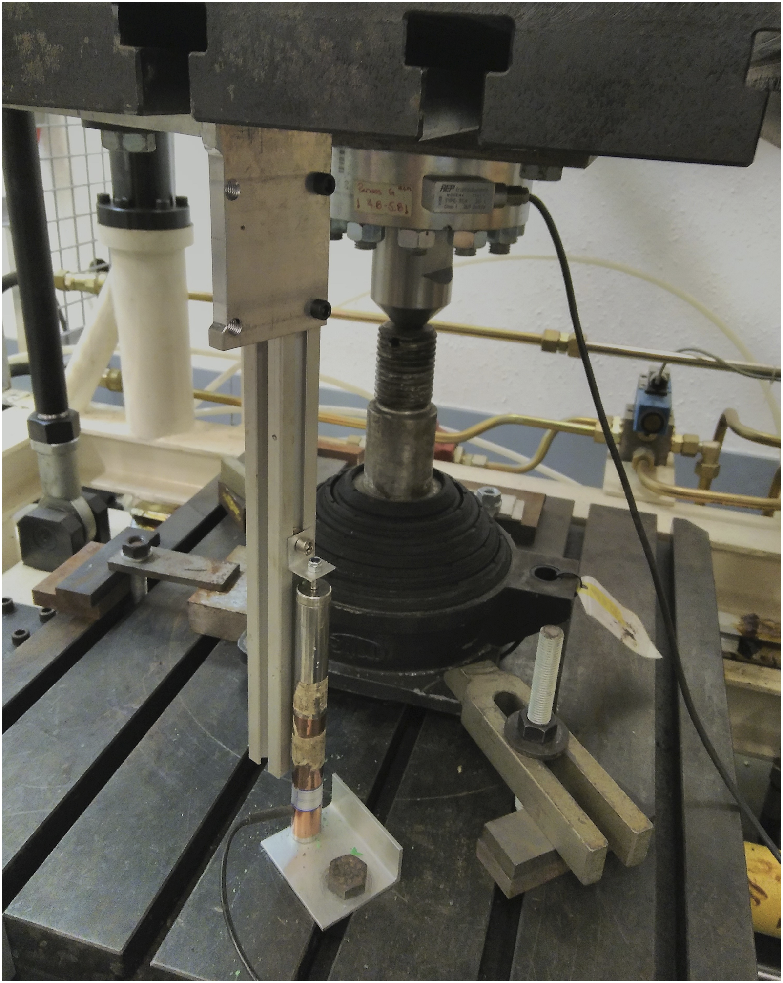

Two different types of tests were carried out: quasi-static tests between zero and the admissible maximum operating load at 50 mm/min deformation speed, and dynamic tests around a specific operation load at frequencies 0.1, 1, 2 and 5 Hz, and amplitudes of 1 and 2 mm. While the former shows the static deformation of the elements at specific loads, from where the required shim thickness can be calculated, the latter offers the possibility to obtain the dynamic stiffness values, which govern the dynamic behaviour in that initial part of the transition. Firstly, the creep results obtained in the quasi-static test will be discussed, and secondly, the results of the dynamic stiffness obtained in the dynamic tests.

Creep and stiffness differences among the elements

Figure 17 shows the load-deformation curve of the quasi-static test of an element in bogie B, normalised with respect to the nominal static curve of a new element. Before recording load and deformation values, at least three pre-conditioning cycles were carried out enabling the rubber to stabilise. The measured loading and unloading curves are slightly different due to the viscoelastic nature of the rubber and the consequent hysteresis energy loss.

Figure 17.

Normalised load-deformation curve of the 50 mm/min quasi-static test for an element in bogie B.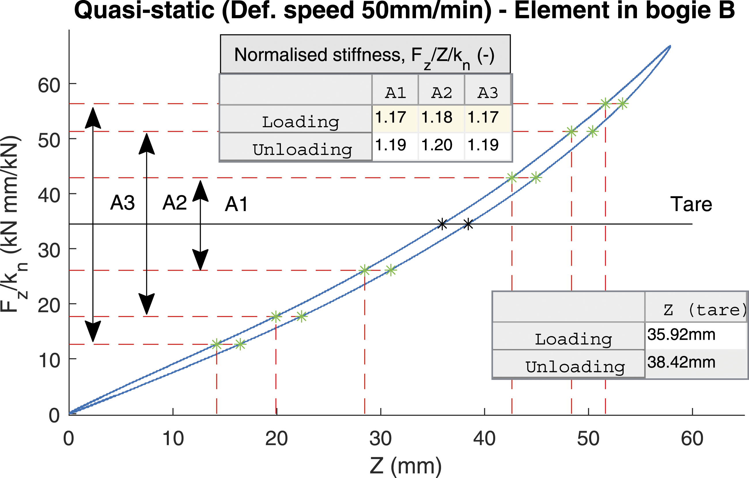

The bottom right table of Figure 17 shows the deformation of the element at the tare load in both the loading and the unloading processes ( $δ_{l}$ and $δ_{u}$ , respectively). From this deformation and the measured initial height of the unloaded element ( $H_{0}$ ), the height under tare load is obtained ( $H_{1}$ ) by equation (3).

H_{1} = H_{0} - δ_{l}

(3)

Then, $H_{1}$ is compared to the tare height tested by the manufacturer at the beginning of each element’s life ( $H_{1}^{n e w}$ ), and the difference calculated as in equation (4) gives the required shim thickness to compensate the height differences ( $t_{r e q .}$ ).

t_{r e q .} = H_{1}^{n e w} - H_{1}

(4)

Then,

t_{r e q .}

can be compared to the real thickness of the introduced shims (

t_{r e a l}

) in each element, where their differences show the additional gauge requirements,

t_{d i f f .} = t_{r e q .} - t_{r e a l}

, and allow to understand if there were load distribution problems caused by those height differences. Table 2 shows

t_{r e a l}

t_{r e q .}

and

t_{d i f f .}

Table 2.

Height difference of the tested elements under tare load accounting for the shims and with respect to the nominal height in tare (mm).

	Bogie A								Bogie B
Wheel	1R		1L		2R		2L		1R		1L		2R		2L
t_req. (mm)	6.7	5.7	6.8	5.5	5.3	6.9	7.3	8.3	9.7	10	9.6	9	5.2	10.2	6.8	7.8
t_real (mm)	5	5	6	6	6	7	8	8	4	4	4	4	2	2	3	3
t_diff. (mm)	1.7	0.7	0.8	−0.5	−0.8	−0.1	−0.7	0.3	5.7	6	5.6	5	3.2	8.2	3.8	4.8

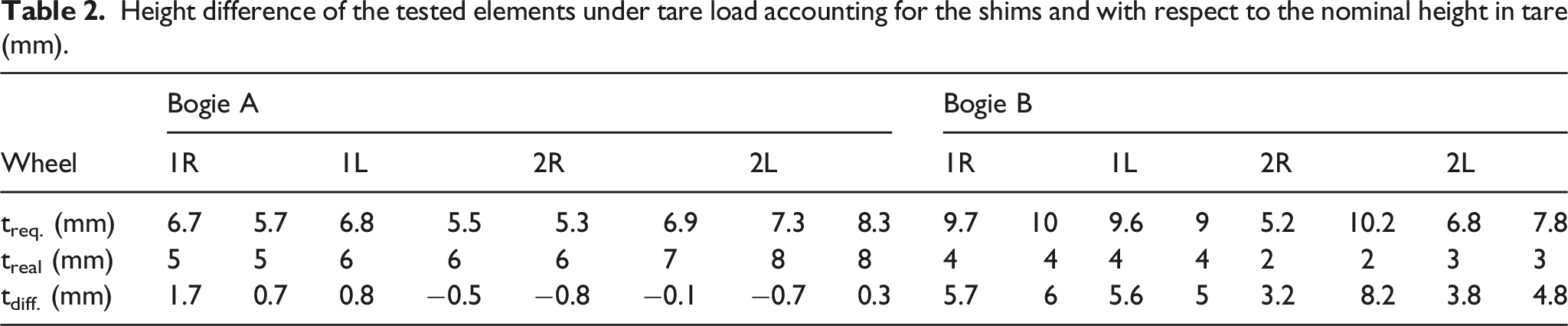
In bogie A all the differences are below 2 mm, which is the minimum shim thickness used in the studied exploitation. Therefore, there were no considerable height differences between the elements when they were installed, as foreseen when applying the developed method to the wayside measurements.

In bogie B the additional gauge requirements, $t_{d i f f .},$ are higher, so that shims should be introduced to keep the differences in line. These results confirm the prognostics inferred from the installed wayside system prototype.

The other cause that can lead to an unbalanced load distribution in the straight is the stiffness difference among the elements. Taking into account that the vertical load variation hardly changes in the straight levelled sections of the railway, the load distribution depends on the static stiffness of the elements rather than the dynamic stiffness, and it can be estimated from the same quasi-static test.

The left upper table in Figure 17 shows the static stiffness increase with respect to the default static stiffness value shown in the plan, calculated both on the loading and unloading curves (the manufacturer recommends the choice of the loading results). For these calculations, three force variations with respect to the tare are used as per the manufacturer’s recommendation: $\pm A 1$ , $\pm A 2$ and $\pm A 3$ (marked with asterisks and dashed lines in Figure 17). The static stiffness increase with respect to the default value provided by manufacturer for the elements of the bogie B are between 16% and 20%, and between 12% and 16% for bogie A. However, the real stiffness value of the elements when they were first installed is unknown, and it is possible that their initial stiffness was already above the value of the plan from the beginning. Moreover, as long as the stiffness values are similar, the static stiffness increase is not such a problem for the dynamic behaviour of the vehicle in circulation, which is more affected by the dynamic stiffness of the suspension. The differences in $F_{1}^{s}$ caused by the expressed stiffness differences are negligible.

Stiffening of the elements

The quasi-static test uses large deformations at low speeds, which does not represent the deformation of the primary suspension in the start of the transition, where the deformation is low and the rate high (it depends on the speed and the cant). The dynamic stiffness of the elements is the parameter governing the behaviour of the primary suspension in this scenario. In order to calculate it, dynamic tests around a specific load were performed. Figure 18 shows the resulting load-deformation dynamic curves of an element in bogie B normalised with respect to the nominal dynamic stiffness values provided by the manufacturer. The hysteresis phenomenon increases with frequency. The little undulations of the curves are probably consequence of a little stick-and-slip effect on the machine guides. As far as the stiffness values are concerned, they barely change with respect to the nominal value, and the same occurs in the rest of the tested elements. This means that the dynamic stiffness of the primary suspension in the bogies where these elements were installed was adequate, and there was no derailment risk due to excessive stiffening. This corroborates the result obtained by the wayside system.

Figure 18.

Normalised load-deformation curves of the dynamic tests for an element in bogie B: (a) 0.1 Hz, 1 mm, (b) 0.1 Hz, 2 mm, (c) 1 Hz, 1 mm, (d) 1 Hz, 2 mm, (e) 2 Hz, 1 mm, (f) 2 Hz, 2 mm, (g) 5 Hz, 1 mm, (h) 5 Hz, 2 mm.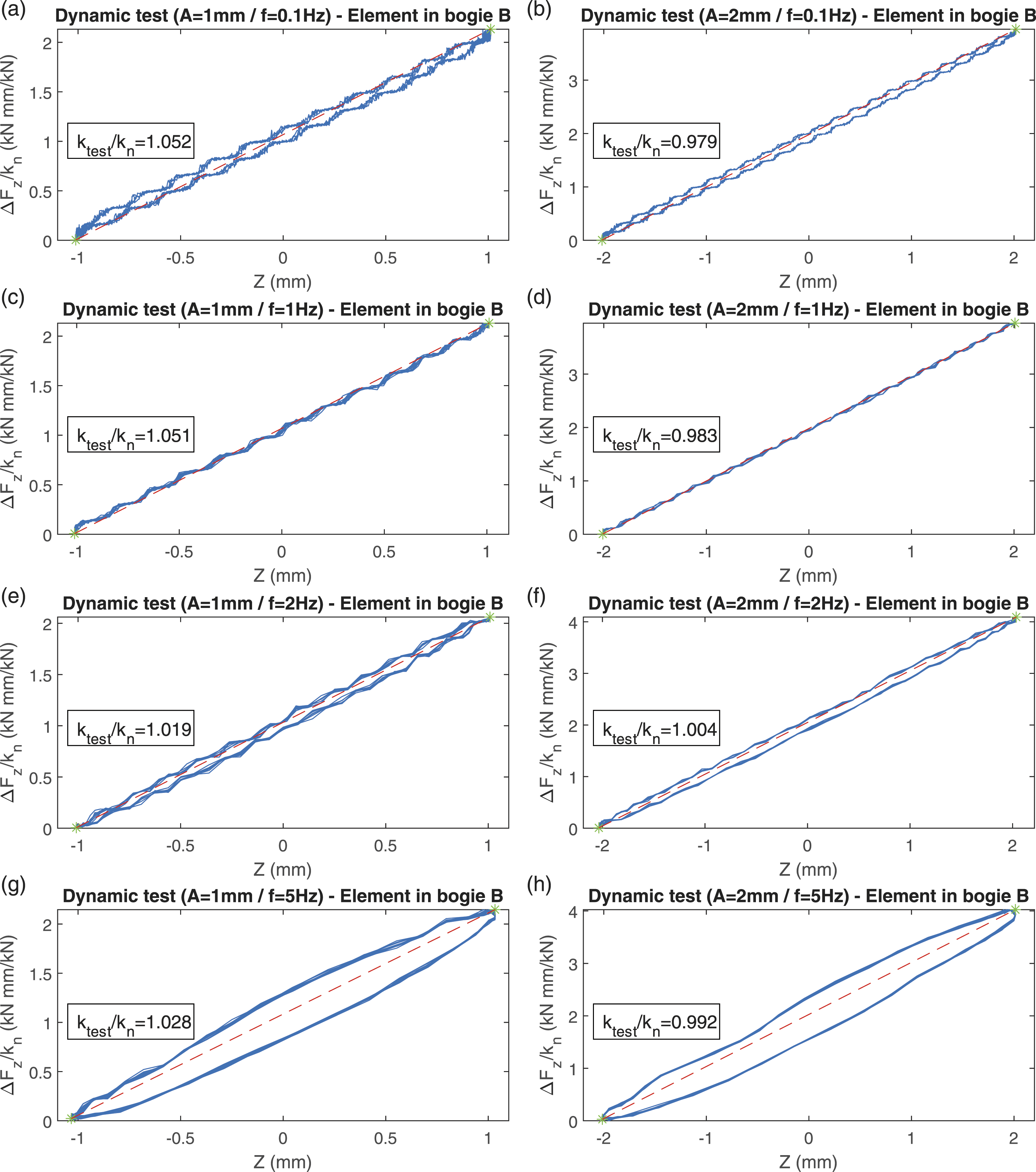

Conclusions

A method to assess the condition of railway vehicles’ primary suspension using wayside measurements of the passing wheel loads at discrete points has been developed. The methodology uses two parameters: the bogie-twist parameter measured on straight track, $F_{1}^{s}$ , and the bogie-twist variation parameter, $∆ F_{1}$ , for a specially identified point located at the beginning of a transition curve. Variations of load and speed do not influence these parameters in those locations, so they directly reflect the condition of the primary suspension.

With both parameters, problems related to creep and stiffening can be detected. When the elements of one bogie have different heights due to creep problems, or when the stiffness of all the elements is not the same, the load is not equally distributed on the wheels and the value of $F_{1}^{s}$ becomes different from zero. Parameter $∆ F_{1}$ , on the other hand, is influenced only by the stiffness of the primary suspension, and thus, unaffected by the height differences produced by creep. When all the elements are stiffened to the same extent, $F_{1}^{s}$ is zero, but there is a variation of $∆ F_{1}$ .

These parameters can be obtained in service and by means of a wayside system. In fact, a prototype has been installed in a metro track monitoring the results for 4 months. This wayside system has proved to be an effective and simple tool to monitor the whole fleet.

Finally, the results of the wayside system have been satisfactorily proven by the thorough laboratory analysis of the individual suspension elements of two monitored bogies. It is concluded that the system can help to assess the condition of the rubber elements in the primary suspension of metro vehicles. Despite focusing on the rubber elements of a metro vehicle, the same methodology might be useful for the assessment of primary suspension systems based on other types of elements.

Footnotes

Declaration of conflicting interests

The author(s) declared no potential conflicts of interest with respect to the research, authorship, and/or publication of this article.

Funding

The author(s) disclosed receipt of the following financial support for the research, authorship, and/or publication of this article: This work was supported by the Bikaintek scholarship from the Basque Government [Grant No. 20-AF-W2-2018-00012], and by the European Union [Grant No., 881807].

ORCID iDs

Ibon Erdozain

Eduardo Gómez

References

Sebesan

Zaharia

Spiroiu

, et al. Rubber suspension, a solution of the future for railway vehicles. Mater Plast 2015; 52(1): 93–96.

Schaefer

. Mechanical properties of rubber. In: Harris

Piersol

(eds). Harris’ Shock and Vibration Handbook. 5th ed. New York: McGraw-Hill, 2002.

Fletcher

Gent

. Nonlinearity in the dynamic properties of vulcanized rubber compounds. Rubber Chem Technol 1954; 27(1): 209–222.

Payne

Whittaker

. Low strain dynamic properties of filled rubbers. Rubber Chem Technol 1971 May 1; 44(2): 440–478.

Mullins

. Softening of rubber by deformation. Rubber Chem Technol 1969; 42(1): 339–362.

Gent

. Relaxation processes in vulcanized rubber. I. Relation among stress relaxation, creep, recovery, and hysteresis. J Appl Polym Sci 1962; 6(22): 433–441.

Stevenson

The influence of low-temperature crystallization on the tensile elastic modulus of natural rubber. J Polym Sci Polym Phys Ed 1983; 21(4): 553–572.

Fuller

KNG

Gough

Thomas

. The effect of low-temperature crystallization on the mechanical behavior of rubber. J Polym Sci Part B Polym Phys 2004; 42(11): 2181–2190.

Teng

Tan

Shi

. Experimental study of high/low temperature effects on the dynamic performance of rubber spring for railway vehicles. J Phys Conf Ser 2019; 1213(5).

10.

Kari

. The non-linear temperature dependent stiffness of precompressed rubber cylinders - An effective shape factor model. Kautschuk Gummi Kunststoffe 2002; 55(3): 76–81.

11.

Chi

Dai

, et al. Calculation of nonlinear stiffness of rubber pad under different temperatures and prepressures. Shock Vib 2020; 2020.

12.

Zhang

Y-R

Zhang

, et al. Primary suspension stiffness testing of railway vehicle bogie. J Jilin Univ (Engineering Technol Ed) 2016; 46(4): 1083–1089.

13.

Johnson

Quigley

Freese

. A viscohyperelastic finite element model for rubber. Comput Methods Appl Mech Eng 1995; 127(1–4): 163–180.

14.

Gil-Negrete

Viñolas

Kari

. A simplified methodology to predict the dynamic stiffness of carbon-black filled rubber isolators using a finite element code. J Sound Vib 2006; 296(4–5): 757–776.

15.

Gil-Negrete

Vinolas

Kari

. A Nonlinear rubber material model combining fractional order viscoelasticity and amplitude dependent effects. J Appl Mech Trans ASME 2009; 76(1): 1–9.

16.

Gajewski

Szczerba

Jemioło

. Modelling of elastomeric bearings with application of Yeoh hyperelastic material model. Procedia Eng 2015; 111: 220–227.

17.

Liu

Yin

Luo

, et al. Finite element analysis and experimental investigation of nonlinear features of rail fastening systems. Proc Inst Mech Eng Part F J Rail Rapid Transit 2018; 232(3): 873–894.

18.

Berg

. A model for rubber springs in the dynamic analysis of rail vehicles. Proc Inst Mech Eng Part F J Rail Rapid Transit 1997; 211(2): 95–108.

19.

Alonso

Gil-Negrete

Nieto

, et al. Development of a rubber component model suitable for being implemented in railway dynamic simulation programs. J Sound Vib 2013; 332(12): 3032–3048.

20.

Shi

. A nonlinear rubber spring model containing fractional derivatives for use in railroad vehicle dynamic analysis. Proc Inst Mech Eng Part F J Rail Rapid Transit 2016; 230(7): 1745–1759.

A condition monitoring approach for the detection of defects in the primary suspension of railway vehicles

Abstract

Keywords

Introduction

Methodology for assessing the assessment of primary suspension condition

Critical parameters

Influence of speed and load

Procedure to determine the condition of the suspension

Approximation of the bogie-twist parameter from discrete load values

Primary suspension condition monitoring system

Primary suspension monitoring system results

Validation of wayside results by detailed experimental tests

Creep and stiffness differences among the elements

Stiffening of the elements

Conclusions

Footnotes

Declaration of conflicting interests

Funding

ORCID iDs

References