Effect of wheel–rail interface parameters on contact stability in explicit finite element analysis

Abstract

It is widely recognized that the accuracy of explicit finite element simulations is sensitive to the choice of interface parameters (i.e. contact stiffness/damping, mesh generation, etc.) and time step sizes. Yet, the effect of these interface parameters on the explicit finite element based solutions of wheel–rail interaction has not been discussed sufficiently in literature. In this paper, the relation between interface parameters and the accuracy of contact solutions is studied. It shows that the wrong choice of these parameters, such as too high/low contact stiffness, coarse mesh, or wrong combination of them, can negatively affect the solution of wheel–rail interactions which manifest in the amplification of contact forces and/or inaccurate contact responses (here called “contact instability”). The phenomena of “contact (in)stabilities” are studied using an explicit finite element model of a wheel rolling over a rail. The accuracy of contact solutions is assessed by analyzing the area of contact patches and the distribution of normal pressure. Also, the guidelines for selections of optimum interface parameters, which guarantee the contact stability and therefore provide an accurate solution, are proposed. The effectiveness of the selected interface parameters is demonstrated through a series of simulations. The results of these simulations are presented and discussed.

Introduction

When performing contact analysis, all contact forces have to be distributed over a priori unknown area in contact. The contact pressure is another primary unknown in such a problem that has to be determined. To estimate these unknowns accurately, extensive research efforts have been made in the field of contact mechanics since the pioneering work of Hertz. ¹ A number of analytical and/or semi-analytical contact solutions, such as Hertzian, ¹ non-Hertzian,^2,3 multi-Hertzian contact models, ⁴ etc., have been developed and reported.^5–7 These approaches have been verified and/or validated to be effective and efficient enough for addressing the problems of wheel–rail (W/R) contact in elasticity as well as in the cases of quasi-static and/or low-frequency dynamics.^2,8–12 Regarding the complex problems with both realistic contact geometries and material plasticity considered, finite element (FE) method, as opposed to the aforementioned approaches, appears to be much preferable and powerful for ensuring the desired solutions.

Generally, two basic methods are used in FE programs to enforce the contact constraints, namely the Lagrange multiplier method^13,14 and the penalty method.^15–18 Due to the easy implementation, the penalty method has been always the first choice to be integrated in the explicit FE software (e.g. ANSYS LS-DYNA ¹⁸ ), where the central difference method is commonly used to perform the time integration.

With the rapid development of computer power and computing techniques, many representative three-dimensional (3D) explicit FE models^19–22 have been created to fulfill different engineering purposes. For instance, Zhao and Li ¹⁹ developed an explicit FE model to study the behavior of W/R frictional rolling contact. The results of verification against CONTACT^3,5 showed that the FE model presented was promising enough to be used in the future work. As a further application of that model presented in Zhao and Li, ¹⁹ Zhao et al. ²² assessed the performance of W/R frictional rolling contact in the presence of rail contaminants. It was reported that contact surface damages such as wheel flats and rail burns might be caused by the presence of contaminants. Vo et al. ²⁰ assessed the stress–strain responses of W/R interaction under high and low adhesion levels. It was found that the adhesion conditions were highly related to the level of damages (RCF damage, corrugation, etc.) on the rail surface. Pletz et al. ²¹ introduced a dynamic wheel/crossing FE model to quantify the influence of the operational parameters such as axle loads, train speeds, etc., on the impact phenomena. It was found that the contact pressure and the micro-slip were critical variables responsible for the surface damage of crossing rail. More recent modeling advances of W/R interaction, including the development of implicit FE models^11,12,23 (i.e. not referenced but of equal importance as those explicit FE models), can be found in Meymand et al. ⁷ and Ma et al. ²⁴

In summary, significant progress in the analyses of W/R interaction using explicit FE tools has been made. However, the issue of selecting good (if not optimum) interface parameters, ¹⁵ as the essence of penalty-type methods, ²⁵ has not been studied sufficiently. Also, the resulting phenomena of “contact instabilities” from the improperly chosen interface parameters have not been discussed adequately. Here, the phenomenon of “contact instability” is referred to as a numerical problem of dynamic contact stability and has no physical correspondence. Detailed explanations of “contact (in)stability” are given in the later sections. The term of “interface parameters” is referred to as the key variables such as contact stiffness and damping that, if changed or varied, influence the entire operation of W/R dynamic interaction system. “Optimum” refers to the “interface parameters” employed that result in acceptable interface compatibility and maintains numerical contact stability. ²⁶

Up until now, only a few general guidelines^{15,18,27–29} are available for making the choice of good interface parameters. For example, Huněk ¹⁵ proposed that an appropriate value of contact stiffness (also called penalty stiffness) can be made considering the penalty stiffness comparable to the normal stiffness of the interface elements. Similarly, Goudreau and Hallquist^18,28 suggested the contact stiffness to be approximately of the same order of magnitude as the stiffness of the elements normal to the contact interface. Belytschko and Neal ²⁷ presented the upper bounds on the contact force in explicit calculations and showed the effect of the contact stiffness on the stable time step. ¹⁵ Pifko et al. ²⁹ introduced a coefficient of contact damping to suppress the high-frequency oscillations.

Although those general guidelines are relatively helpful for identifying good interface parameters, it is widely recognized^{14,15,25,26,30} that there are no universally applicable rules/guidelines for particular problems considered. Regarding the specific problem of W/R rolling contact, more research attention to the importance of interface parameters has to be drawn. The motivation of this study is thus summarized as follows:

To ensure accurate solutions of W/R interaction: Considering that the penalty methods enforce contact constraints approximately, the solution accuracy depends strongly on the interface parameters selected. ¹⁴ A set of arbitrary chosen interface parameters on the risk of being underestimated or overestimated may easily cause an unexpected or inaccurate solution from FE simulations.

To formulate clear guidelines for good W/R interface parameters: The choice of interface parameters can affect not only the accuracy of contact solutions, but also the stability of explicit FE time integration (i.e. central difference method is conditionally stable).^25,26 Thus, well-demonstrated guidelines are in high demand to address the problems of contact instabilities and to maintain the solution accuracy.

To carry out the study on the problems of contact (in)stabilities, an explicit FE model of a wheel rolling over a rail is used. The model adopted is developed in ANSYS LS-DYNA. ¹⁸ To improve the performance of FE simulations on W/R interaction, ²⁴ a novel adaptive mesh refinement procedure based on the 2D geometrical contact analysis is introduced. Also, the accuracy of that model has been successfully verified ³¹ against CONTACT, which is a rigorous and well-established computational program developed by Professor Kalker ⁵ and powered by VORtech Computing. ³ The modeling strategy proposed ²⁴ has been further extended to study the dynamic impact between wheel and crossing. ³²

In this paper, the attention is focused on a comprehensive study on the relation among the choice of interface parameters, the accuracy of contact solutions, and the numerical contact stability. The outline of this paper is as follows. A brief introduction of the explicit FE model developed for the analysis of W/R interaction is presented first. Next section is concentrated on the theoretical background of the FE algorithms to better understand the physics of contact problems before attempting to solve it. Also, the challenges and approaches for maintaining contact stabilities are illustrated. Then, the influence of interface parameters on the computational accuracy and contact stabilities is studied and discussed. Finally, concluding remarks are drawn.

W/R 3D-FE model

In this section, the FE model for the analysis of W/R interaction is presented. The model is shown in Figure 1(a) to (f). The two counterparts investigated here are the standard S1002 wheel and the 54E1 rail, which are commonly used in the Dutch railway network. Note that the model can easily be adjusted for other wheel and rail profiles (i.e. measured worn profiles, UIC60, UIC75, etc.). The single rail instead of a complete track (i.e. double rails) is modeled by taking advantage of the symmetrical characteristic of the vehicle and track. In order to reduce the calculation expense, a short rail length of 1.8 m is selected as inspired by Vo et al. ²⁰ and Pletz et al. ²¹ The two ends of rail are constrained in the longitudinal and lateral directions. The bottom surface of rail is completely fixed (i.e. a rigid foundation as inspired by the work of Zhao and Li ¹⁹ ). The reason for defining such boundary conditions is to minimize the vibration of the structure (e.g. the sprung mass in Figure 1(a)) excited by the rolling of a wheel over a rail. In this way, the comparability of FE results to those of CONTACT, which focuses on the cases of steady-state contact,^5,33 can be enhanced for the purpose of verification.^19,31 The results of the verification of FE model with realistic W/R profiles considered have already been presented in Ma et al. ³¹

Figure 1.

FE model of W/R dynamic contact: (a) schematic graph; (b) FE model – side view; (c) refined mesh at the rail potential contact area; (d) refined mesh at the wheel potential contact area; (e) FE model – cross-sectional view; (f) close-up view in refined regions.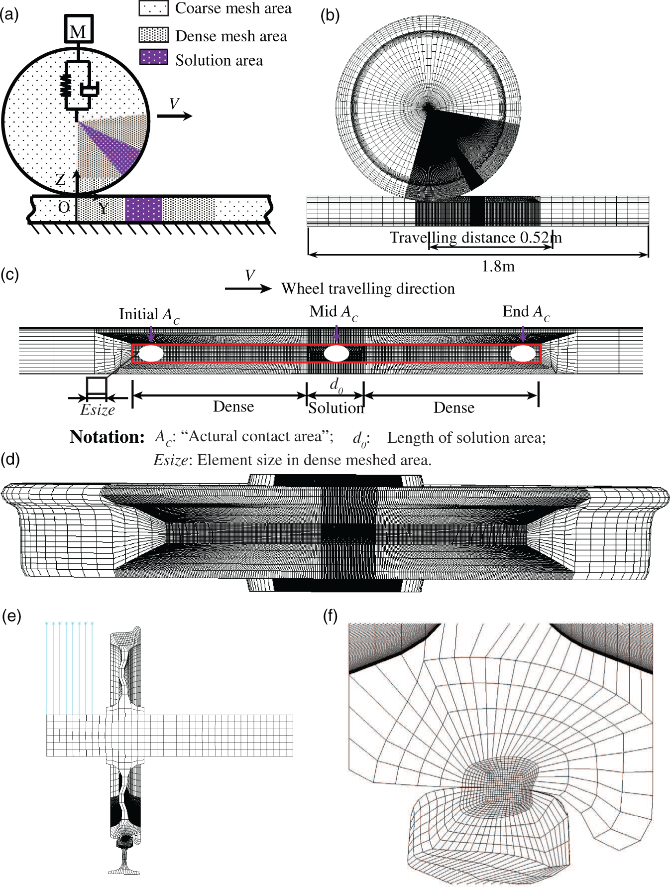

The wheel is set to roll from the origin of the global coordinate system over a short traveling distance of 0.52 m along the rail (see Figure 1(a) and (b)). The corresponding wheel rolling angle (i.e. a wheel rolled) is approximately 65°. The wheel is traveling with an initial translational velocity of 140 km/h (typical speed of VIRM intercity trains in the Netherlands). Accordingly, an initial angular velocity of 84.46°/s (based on the magnitudes of wheel rolling radii) is exerted on the wheel. Besides, a driving torque with a traction coefficient of 0.25 is applied on the wheel.

The global coordinate system O – XYZ is defined as: the X-axis is parallel to the longitudinal direction along which the wheel-set travels, the Z-axis is the vertical pointing upwards, and the Y-axis is perpendicular both X and Z directions, forming a right-handed Cartesian coordinate system.

In the FE model, the wheel and rail contact bodies are discretized with 3D 8-node structural solid elements (SOLID164). Only the regions where the wheel travels are discretized with the dense mesh, leaving the remaining regions with the coarse mesh (see Figure 1(a) to (d)). A solution area is introduced and positioned in the middle of the dense meshed area. This area is defined as a region to extract and analyze the contact properties, such as the resulting contact patch and normal pressure. In this region, the mesh size is approximately two times smaller than the dense meshed area for the purpose of capturing the high stress–strain gradients. For the FE model shown in Figure 1, the mesh size in the solution area is 1 mm, while that in the dense meshed area is 2 mm. The wheel model has 141,312 solid elements and 154,711 nodes, whereas the rail model has 117,598 solid elements and 132,177 nodes.

To take the primary suspension system into account, a group of sprung mass blocks are lumped over the spring-damper system. The mass blocks, which are used to represent the weight of the loaded car body, have the weight of 10 tons. The corresponding parameters of the springs and dampers are listed in Table 1. The linear elastic material model is used to describe the constitutive relation of the wheel and rail components. ²⁴

Table 1.

Material properties and mechanical parameters.

	Properties	Values
Wheel–rail material	Young modulus (GPa)	210
	Poisson’s ratio	0.3
	Density (kg/m3)	7900
Primary suspension	Stiffness (MN/m)	1.15
	Damping (Ns/m)	2500
Operational parameters	Friction coefficient a	0.5
	Traction coefficient b	0.25
	Train velocities (km/h)	140

a

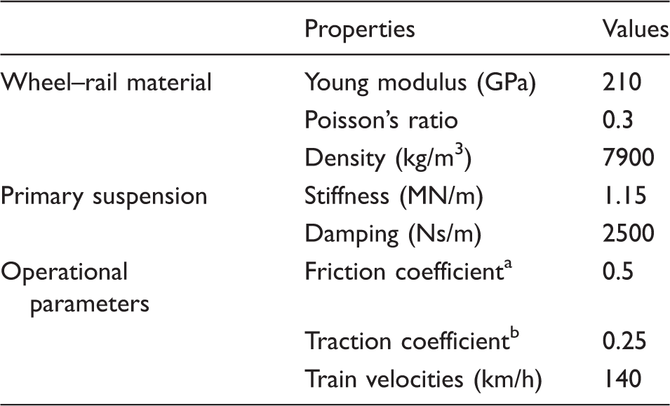
Friction is the force resisting the relative motion (i.e. slip) of contact surfaces. Coefficient of friction = Friction force/Normal force.

b

Traction is the force applied to generate motion between a body and a tangential surface. The tangential traction appears only if the friction is assumed. Coefficient of traction = Traction/Normal force.

For such a typical FE contact analysis, the basic process consists of three steps: (1) Build the model, prescribing the initial location of W/R, defining correct boundary conditions, and preforming mesh refinement; (2) Apply axle loads and run simulations, involving traction application, contact definition, and settings of time steps; (3) Post-process the FE simulation results, examining the contact properties such as normal pressure, shear stresses within the contact patch, subsurface stress–strain responses, etc.

All the explicit FE simulations are performed on a workstation with an Intel(R) Xeon(R) @ 3.10 GHz 16 cores CPU and 32 GB RAM. Also, the shared memory parallel processing capability of ANSYS LS-DYNA (high-performance computation module) for eight processors is used.

Recap explicit FE theory

In this section, the corresponding explicit FE theories, which are highly related to the background of contact stability, are recapitulated. More generally, a solution of the unknown vector of the displacements $\stackrel{\sim }{\mathbf{u}}$ is to be found through the process of FE analysis. Using the Galerkin approximation method, ³⁴ the discretized equation of motion is given as ³⁵

$$\stackrel{\mathrm{··}}{\stackrel{\sim }{\mathbf{M}}}\mathbf{u}=\mathbf{Ma}=\mathbf{F}$$

(1)

where M is the mass matrix, F is the force vector, and a is the nodal acceleration vector.

Stability of central difference method

By taking advantage of the central difference method,^18,30,35 the iterative scheme of the explicit time integration varying from the instant t_n to $t_{n+1}$ becomes ¹⁸

$$\begin{array}{c}\multicolumn{1}{c}{\begin{array}{c}{\mathbf{a}}_n={\mathbf{M}}^{-1}{\mathbf{F}}_n\\ {\mathbf{V}}_{\frac{n+1}{2}}={\mathbf{V}}_{\frac{n-1}{2}}+{\mathbf{a}}_n\Delta t_n\\ {\mathbf{u}}_{n+1}={\mathbf{u}}_n+{\mathbf{V}}_{\frac{n+1}{2}}\Delta t_{\frac{n+1}{2}}\end{array}}\end{array}$$

(2)

where $\Delta t_{\frac{n+1}{2}}=\frac{(\Delta t_n+\Delta t_{n+1})}{2}$ . V is the global nodal velocity vector and n indicates the number of time steps. Due to the conditionally stable characteristic of the central difference method, the integration time step $\Delta t_{\mathit{calc}}$ (also called the calculation time step) must be small enough to maintain the numerical stability of the solution. The exact stability criteria is expressed as^18,30

$$\Delta t_{\mathit{calc}}<\Delta t_{\mathit{crit}}=2/{\omega }_{\text{max}}$$

(3)

where ω_max denotes the maximum eigenfrequency in the FE model. To satisfy these stability criteria, the explicit FE solver needs to find the maximum eigenfrequency of the whole FE dynamic system. As reported in Hallquist ¹⁸ and Wu and Gu, ³⁵ this is not practical, not only due to the computational cost but also the lack of Eigen-solver in the explicit FE program. The alternative of equation (3) is the Courant–Friedrichs–Lewy stability criteria (also called the Courant criteria), ³⁶ which states

$$\Delta t_{\mathit{calc}}=\text{min}\{\Delta t_1,\Delta t_2,\Delta t_3,\dots ,\Delta t_N\}$$

(4)

From Courant criteria, it can be seen that the global calculated time step $\Delta t_{\mathit{calc}}$ is determined on the basis of the smallest critical time step value of all the elements within the FE model. Here, N refers to the maximum number of the element in the FE model.

Penalty method

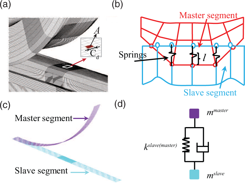
The penalty method^17,30 is one of the most commonly used approaches to enforce the contact constrains in the explicit FE programs, where a list of invisible “interface spring” elements are placed between the penetrating slave nodes and the master segments (as depicted in Figure 2(a) to (c)). The restoring interface force vector ${\mathbf{f}}_s$ ¹⁷ is aligned with the normal of the master segment ${\mathbf{n}}_i$ and linearly dependent on the penetration depth l

$$\mathit{Ifl}<0,{\mathbf{f}}_s=-l·k·\mathbf{n}$$

(5)

Figure 2.

Schematic graph of the penalty method: (a) close-up view of FE model; (b) cross-sectional view of the contact segments; (c) master–slave segments; (d) schematic of the “invisible” spring-damper-mass system.

Contact stiffness

The penalty stiffness k for these “springs” is prescribed as follows ¹⁸

$$k=\frac{\alpha ·K·A^2}{V}=\alpha ·K·C_d$$

(6)

where α denotes the penalty scale factor, K is the bulk modulus, V and A represent the volume and face area of a contact element respectively, and C_d is the side length of this element. An example of such a contact element is shown in Figure 2(a).

Contact damping

In order to avoid undesirable oscillations in contact, a certain amount of damping perpendicular to the contact surfaces is automatically included in the explicit FE software (e.g. LS-DYNA). For simplicity, a damping coefficient ξ is introduced as ¹⁸

$$\xi =\frac{\mathit{VDC}}{100}{\xi }_{\mathit{crit}}$$

(7)

where ξ is given in percent of the critical damping coefficient ξ_crit for explicit contact. VDC is the abbreviation of “viscous damping coefficient in percent of critical”. By default, ¹⁸ the magnitude of VDC is 80, which means the applied damping coefficient ξ is as large as 80% of the critical damping coefficient ξ_crit. VDC is a control parameter that can be tuned to fit particular contact-related problems.

Contact stability

Together with the related nodal mass m^master and m^slave, the “closed” contact segment (see Figure 2) becomes an “invisible” spring-damper-mass system. Here, the contact segments are the components of nodes on the outmost surface layer of the two wheel–rail contact bodies (see Figure 1 and Figure 2(c)). m^master and m^slave are referred to as the master and slave nodal mass, respectively.

The interface spring stiffness k used in the contact algorithms ¹⁸ is based on the minimum value of the slave segment stiffness k^slave or master segment stiffness k^master. Accordingly, there are two time step sizes obtained according to the two contact stiffness (master and slave) for these invisible spring-damper contact elements. One is the contact time step size of the master segment, and the other is that of the slave segment.

Contact surface time steps

Two critical time steps for the master segments 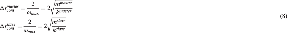$\Delta t_{\mathit{cont}}^{\mathit{master}}$ and the slave segments $\Delta t_{\mathit{cont}}^{\mathit{slave}}$ are defined individually as ¹⁸

$$\begin{array}{c}\multicolumn{1}{c}{\begin{array}{c}\Delta t_{\mathit{cont}}^{\mathit{master}}=\frac{2}{{\omega }_{\text{max}}}=2\sqrt{\frac{m^{\mathit{master}}}{k^{\mathit{master}}}}\\ \Delta t_{\mathit{cont}}^{\mathit{slave}}=\frac{2}{{\omega }_{\text{max}}}=2\sqrt{\frac{m^{\mathit{slave}}}{k^{\mathit{slave}}}}\end{array}}\end{array}$$

(8)

Taking the contact damping coefficient ξ into account, the critical time step size of contact elements $\Delta t_{\mathit{cont}}^{\mathit{master}}$ and $\Delta t_{\mathit{cont}}^{\mathit{slave}}$ will be reduced as ¹⁸

$$\Delta t_{\mathit{cont}}^{\mathit{master}(\mathit{slave})}=2\sqrt{\frac{m^{\mathit{master}(\mathit{slave})}}{k^{\mathit{master}(\mathit{slave})}}}(\sqrt{1+{\xi }^2}-\xi )$$

(9)

Contact stability criteria

The calculation time step $\Delta t_{\mathit{calc}}$ used in the explicit FE software (e.g. LS-DYNA) is not allowed to be larger than the critical contact surface time step sizes, ¹⁸ i.e.

$$\Delta t_{\mathit{calc}}<\text{min}(\Delta t_{\mathit{cont}}^{\mathit{master}},\Delta t_{\mathit{cont}}^{\mathit{slave}})$$

(10)

Otherwise, the contact stability could not be guaranteed.

Underlying challenges and possible solutions

As it has been presented in the section “Recap explicit FE theory”, the FE theoretical background is rather complicated. There are several interface parameters involved in both the contact modeling and solving procedures. Thus, a number of challenges are encountered and need to be addressed.

Interface parameters

To properly capture the highly nonlinear contact characteristics of W/R interaction, a very dense mesh in the potential contact area is always desired. However, it is not always the case that the very dense mesh can be used in the model due to the large and complex contact geometries as well as the limited computer capability. Therefore, a nonuniform mesh (see Figure 1(c)) is introduced by making the solution area much denser than the other contact regions.

It is clear that the two parameters (mesh density and mesh uniformity) shown in Figure 1(c) are to be adjusted and evaluated. By decreasing the length d₀ of the solution area into zero, the nonuniform mesh refinement becomes a uniform one. Similarly, the mesh density could be changed by increasing or decreasing the mesh size Esize of the element. Here, “mesh density” refers to the number of elements per unit area in the dense meshed area (not that in the solution area).

Besides, there are no standard routines on how to prescribe the magnitude of the penalty scale factor α and the contact damping factor VDC embedded in equations (6) and (7). Their effects on the contact stability have not been sufficiently discussed especially in the field of FE-based simulations on W/R rolling frictional contact.

To sum up, the main challenges associated are exploring the relation between the dynamic responses of W/R interaction and the four key interface parameters: namely, (1) Penalty scale factor α; (2) Mesh uniformity d₀; (3) Mesh size Esize; (4) Contact damping factor VDC.

Approaches for addressing challenges

To address the aforementioned challenges, the approach of parametric study is adopted. In this section, the details of this approach are given first. Following that, the scheme on how to integrate such an approach with the FE analysis is reported.

Parametric study

According to the general rule of a parametric study, the dynamic behavior of the W/R interaction has to be studied by iteratively varying the values of certain interface parameters, while the other parameters are fixed. Based on the parametric studies, the following questions are expected to be answered:

How does the contact instability look like? Are there any effective measures for maintaining the contact stability (if contact instability happens)?

What are the effects of the interface parameters on the performance of the contact stability as well as on the dynamic contact responses?

Is there a set of interface parameters that is the most suitable one for the analysis of W/R interaction?

Integration with FE model

To perform the parametric study, it has to be properly integrated with the 3D-FE model. Its basic working mechanism is shown in Figure 3.

Figure 3.

Flow chart of the parametric study with 3D-FE model.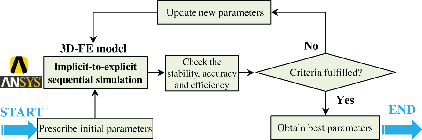

Firstly, an initial set of the interface parameters is prescribed in the 3D-FE model. Once the explicit FE simulations are completed, the statuses of the contact stability, calculation efficiency, and accuracy have to be examined. The criteria are the good compromise among the contact stability, calculation efficiency, and accuracy. When the criteria are satisfied, the best set of the interface parameters is identified. If not, new parameters will be updated and tested against the 3D-FE simulations iteratively until such a compromise is reached.

Results and discussions

Following the flow chart shown in Figure 3, a series of explicit FE simulations are performed so as to examine the effect of the four interface parameters on the performance of W/R interaction. These interface parameters vary within certain given ranges:

Penalty scale factor α (from 0.05 to 409.6);

Mesh uniformity d₀ (from 0 mm to 120 mm);

Mesh size Esize (from 1.5 mm to 4.0 mm);

Damping factor VDC (from 10 to 180).

It is worth noting that all these interface parameters are studied in the case of zero lateral shift of the wheel-set. To increase the calculation efficiency of this parametric study, the FE modeling procedure has been parameterized using MATLAB scripts and ANSYS Parametric Design Language (APDL). ²⁴

Contact stiffness

Nine cases of penalty scale factor varying from 0.05 to 102.4 are selected for analysis, while the other parameters are kept constant. Due to the inversely proportional relation between the contact time steps $\Delta t_{\mathit{cont}}^{\mathit{slave}(\mathit{master})}$ and the square root of the penalty scale factor α (equations (6) and (8)), the increase of penalty scale factor α will lead to the decrease of contact time step $\Delta t_{\mathit{cont}}^{\mathit{slave}(\mathit{master})}$ . The values of penalty scale factors are thus set to be the product of its “default” (0.1) and the mth power of 2 (i.e. $\alpha =0.1\times 2^m$ ), which is to maintain the variation of $\Delta t_{\mathit{cont}}^{\mathit{master}}$ and $\Delta t_{\mathit{cont}}^{\mathit{slave}}$ to be approximately linear. m is chosen to be in the range of [−1, 10]. Here, the term of “default” means the program suggested settings in explicit FE software LS-DYNA. In this way, the influence of penalty scale factors on the contact stability (equation (10)) is able to be effectively investigated.

Figure 4(a) shows the variation of vertical contact forces corresponding to different penalty scale factors α. It can be seen that a “saw-toothed” force oscillation is generated and located at a distance of 150 mm from the origin. As the wheel rolls further along the rail and approaches the vicinity of the solution area (d₀ = 80 mm), a “sudden perturbation” of the contact force gets noticeable for the cases of α = 204.8 and α = 409.6 (extremely high contact stiffness) as well as those of α = 0.05 and α = 0.1 (extremely low contact stiffness).

Figure 4.

(a) Variation of the vertical contact forces w.r.t. different penalty scale factors α; (b) variation of three typical time steps.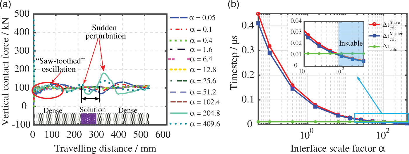

The observed “saw-toothed oscillations” and “sudden perturbations” of the contact forces could all be interpreted as the indicators of “contact instability”. In contrast, a continuous and smooth dynamic response from the explicit FE simulations is perceived as a prognosis of the “contact stability”.

A comparison (see Figure 4(b)) of the contact time steps $\Delta t_{\mathit{cont}}^{\mathit{master}},\Delta t_{\mathit{cont}}^{\mathit{slave}}$ with the calculation time step $\Delta t_{\mathit{calc}}$ has been performed for all the studied cases. It shows that the two critical contact time step sizes $\Delta t_{\mathit{cont}}^{\mathit{master}}$ and $\Delta t_{\mathit{cont}}^{\mathit{slave}}$ decrease significantly with the increase of the penalty scale factor α. At the region denoted by the red block, where the penalty scale factor α is larger than 100, the calculation time step $\Delta t_{\mathit{calc}}$ starts to exceed the thresholds of the critical contact time steps $\Delta t_{\mathit{cont}}^{\mathit{master}}$ and $\Delta t_{\mathit{cont}}^{\mathit{slave}}$ . According to equation (10), such a violation of the time step inequality could be hypothesized to be the main cause of the “sudden perturbation” at the solution area for the cases of $\alpha =204.8$ and $\alpha =409.6$ . With regard to the “saw-toothed oscillations”, it is hypothesized to be caused by the initial conditions (i.e. the vibration of the structure excited by the initial train velocities, see Table 1) of the explicit FE analysis.

In order to verify the hypothesis of the initial conditions, four FE simulations with different initial train velocities V₀ ranging from 90 km/h to 250 km/h are performed. Here, the penalty scale factor α of 12.8 is adopted. Figure 5(a) shows the variation of vertical contact forces with respect to different initial train velocities V₀. At the higher train speed levels, it can be seen that the “saw-toothed” dynamic force oscillations are getting more noticeable.

Figure 5.

(a) Variation of the vertical contact forces w.r.t. different train velocities V₀; (b) variation of the vertical contact forces corresponding to reduced calculation time step sizes 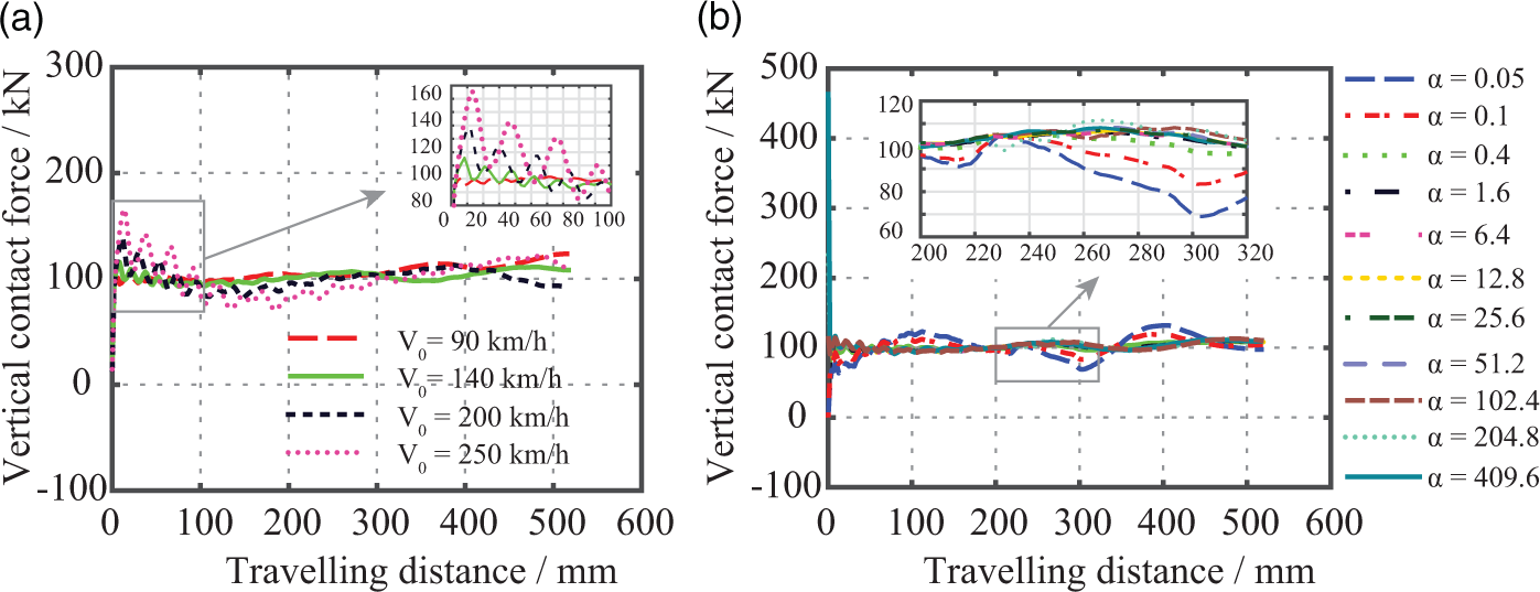$\Delta t_{\mathit{calc}}$ .

Besides, two more FE simulations for the cases of $\alpha =204.8$ and $\alpha =409.6$ have been performed, where their calculation time step sizes $\Delta t_{\mathit{calc}}$ have been scaled down with a factor of 0.5 and 0.15, respectively. The corresponding variation of vertical contact forces is shown in Figure 5(b). It can be clearly seen that the “sudden perturbations” at the vicinity of the solution area have disappeared. Thus, the two hypotheses of the time steps violations and initial conditions have been verified.

However, the calculation expenses for the tuned cases of $\alpha =204.8$ and $\alpha =409.6$ , which grow from 8.8 h to 15.91 h and 50.32 h, have been significantly increased because of the reduced calculation time step size. As a consequence, the calculation efficiency is negatively affected. Moreover, it is observed from Figure 5(b) that the variation of vertical contact forces is getting converged with the increase of the penalty scale factor α.

Figure 6 shows the distributions of normal contact pressure, which are extracted at the instant when the wheel travels over the middle of the solution area. It can be seen that both the magnitude and distribution of the contact pressure tend to converge at higher levels of penalty scale factor. Such an observation agrees well with the classical penalty theory^17,18,30,34 that the larger the contact stiffness is, the more realistic the results would be.

Figure 6.

Effect of contact stiffness on contact pressure distribution.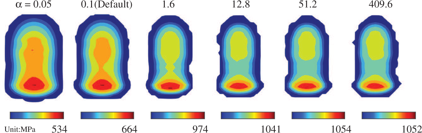

It can be concluded from the simulation results that the default parameters (such as the default penalty scale factor α = 0.1) in LS-DYNA cannot accurately simulate the dynamic behavior of the W/R interaction well, and the values of these parameters used in the analysis have to be justified. The guidelines for selecting a suitable penalty scale factor α could be formulated as follows:

To ensure a proper accuracy of the contact solution, the contact stiffness should be as large as possible, which can be achieved by increasing the penalty scale factor α. For the chosen value of the penalty scale factor, the calculation time step $\Delta t_{\mathit{calc}}$ should be smaller than the contact time step sizes $\Delta t_{\mathit{cont}}^{\mathit{slave}(\mathit{master})}$ so as to guarantee the contact stability as explained in Figure 4. The time step sizes of $\Delta t_{\mathit{cont}}^{\mathit{slave}(\mathit{master})}$ are available in the output of LS-DYNA;

Once the calculation time step $\Delta t_{\mathit{calc}}$ exceeds the thresholds of contact time steps $\Delta t_{\mathit{cont}}^{\mathit{slave}(\mathit{master})}$ , a reduced calculation time step is demanded to retrieve the stable dynamic contact response and get rid of the sudden perturbations (if it happens), but with a sacrifice of the calculation efficiency.

Based on the aforementioned guideline, a penalty scale factor α of 12.8 that can maintain the best compromise of the accurate contact performance and calculation efficiency is suggested.

Mesh uniformity

Figure 7(a) and (b) shows the FE models corresponding to different mesh uniformities. The case of d₀ equal to 0 mm indicates the uniform mesh (see Figure 7(d)). d₀ is prescribed to vary from 0 mm to 120 mm. When the length of the solution area changes from 40 mm to 120 mm, the number of the solid elements in the solution area increases from 472 to 1382.

Figure 7.

Variation of nonuniform mesh to uniform mesh: (a) 120 mm; (b) 80 mm; (c) 40 mm; (d) 0 mm – uniform mesh.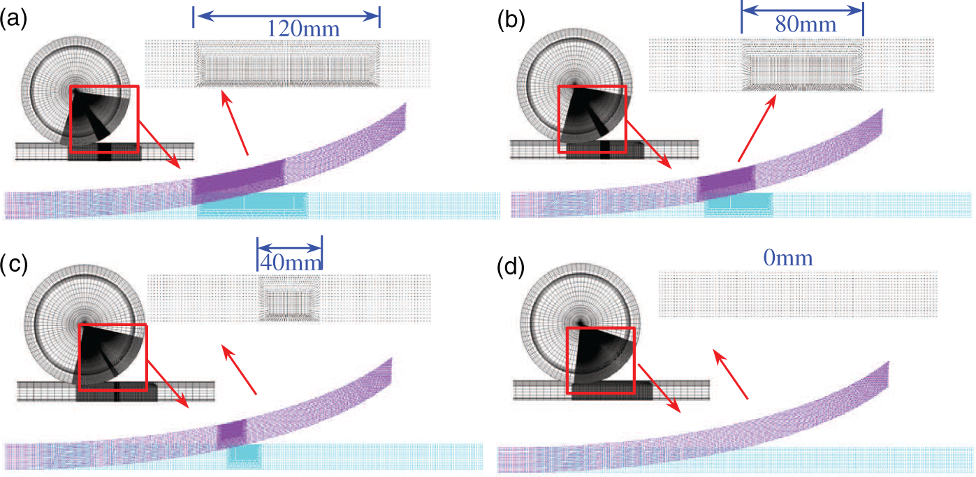

To study the influence of the mesh uniformity on the dynamic performance of W/R interaction, the default penalty scale factor α of 0.1 is chosen to be studied first, while the other parameters (except the mesh uniformity d₀) are fixed.

Figure 8(a) shows the dynamic responses with the default penalty scale factor of $\alpha =0.1$ . It can be noticed that the “sudden perturbations” happen again nearby the solution area. Taking the case of d₀ = 0 mm (uniform mesh refinement) as a reference, it can be seen that the location of the starting and ending points of the perturbation is highly related to the exact position and the dimension d₀ of the solution area. Moreover, it can be observed that the curves of the vertical contact forces are overlapped before the wheel enters into the solution area, while the difference gets more pronounced after it passes over the solution area. Presumably, it is the default penalty scale factor $\alpha =0.1$ that is too low to compensate the drastic contact stiffness difference between the dense meshed region and the solution area of the contact bodies as shown in Figure 8(a).

Figure 8.

Variation of the vertical contact forces w.r.t. different mesh uniformities: (a) default penalty scale factor 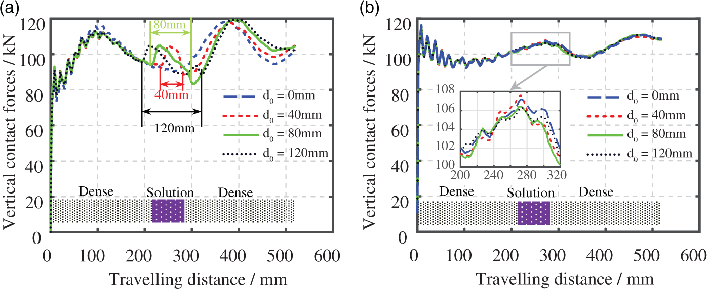$\alpha =0.1$ ; (b) optimal penalty scale factor $\alpha =12.8$ .

To verify the presumption of the contact stiffness difference, another four cases of FE simulations corresponding to different mesh uniformities have been analyzed using the suggested best penalty scale factor of 12.8. The variation of the vertical contact forces is shown in Figure 8(b). It can be seen that the “sudden perturbations” of the contact instability inside the solution area, which occur at the default penalty scale factor of 0.1 as shown in Figure 8(a), die out. All the responses of the contact forces seem to converge into a common curve. This implies that the “sudden perturbations” introduced by mesh nonuniformity at low contact stiffness could be arrested and eliminated by specifying a high enough penalty scale factor (i.e. 12.8). In other words, the high penalty scale factor can minimize the contact stiffness difference and maintain the contact stability.

Figure 9 shows the variation of time step sizes corresponding to different mesh uniformities. It is clear that the calculation time step size $\Delta t_{\mathit{calc}}$ decreases significantly, when the mesh pattern changes from uniform to nonuniform. For this reason, the calculation expense of the nonuniform mesh increases from 8 h (in comparison to that of the uniform mesh) to more than 20 h. Besides, it is observed that, at higher penalty scale factor of $\alpha =12.8$ , the gap between calculation and contact time step sizes reduces much more than that of the low penalty scale factor ( $\alpha =0.1$ ). This is complementary to the relation between contact stiffness and the time step size as derived from equation (8).

Figure 9.

Variation of time step sizes w.r.t. different mesh uniformities: (a) default penalty scale factor 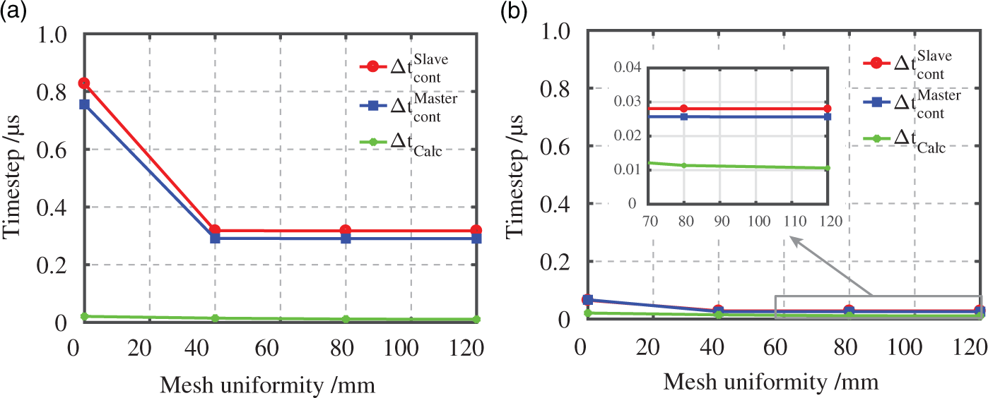$\alpha =0.1$ ; (b) optimal penalty scale factor $\alpha =12.8$ .

It is observed from Figure 10 that both the magnitude and distribution of the contact pressure obtained from the uniformly meshed FE model are quite different from those of the FE simulations having nonuniform mesh patterns. The reason for that is attributed to the difference of FE mesh patterns in the solution area, where the uniformly meshed FE model is too coarse to capture the high stress gradients within the contact patch. It further demonstrates the importance of mesh nonuniformities to the contact solutions, which means the mesh nonuniformity is one necessary feature for the analysis of W/R interaction.

Figure 10.

Effect of mesh uniformity on contact pressure distribution.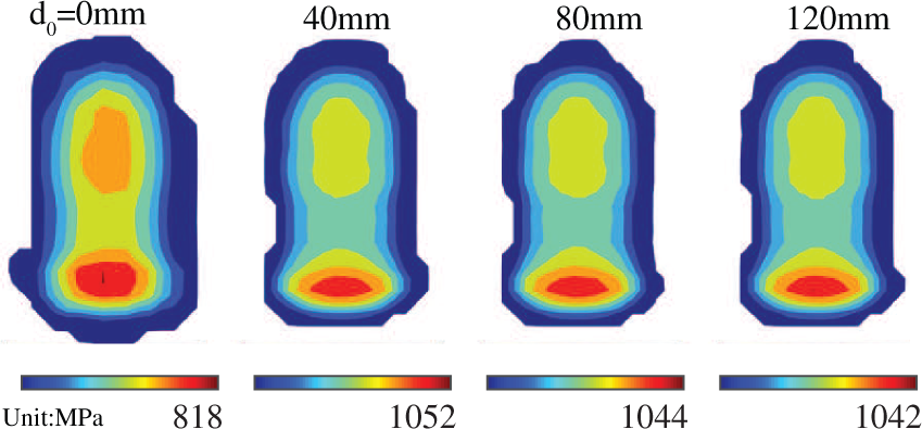

Although the mesh nonuniformity can introduce a high calculation expense compared with the uniformed mesh, detailed contact properties are obtained. Considering that the longer the refined solution area is, the greater the amount of the elements will be created, it makes sense to adopt the length d₀ = 80 mm of the solution area to make a good compromise between the calculation efficiency and accuracy. Although the mesh nonuniformity introduces contact instability, using proper contact stiffness this effect can be eliminated.

Mesh density

In order to study the effect of mesh density on the performance of W/R interaction, six cases of mesh size varying from 1.5 to 4.0 mm are studied. The other parameters are fixed.

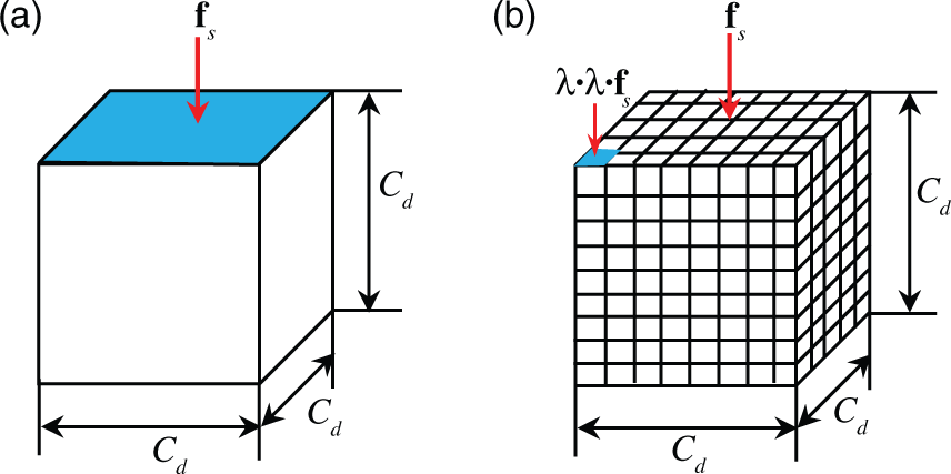
Figure 11(a) shows the variation of vertical contact forces corresponding to different mesh sizes. It should be noted that the penalty scale factor $\alpha =0.1$ is in default for the present studied cases. It can be seen that the amplitude of “sudden perturbations” inside the solution area gradually reduces with the decrease of the mesh size. It implies that the mesh density would be an alternative parameter for preventing the “sudden perturbations” in addition to the penalty scale factor α.

Figure 11.

Variation of the vertical contact forces w.r.t. different mesh sizes: (a) default penalty scale factor $\alpha =0.1$ ; (b) optimal penalty scale factor $\alpha =12.8$ .

Figure 12.

Schematic graph of the mesh size variation: (a) brick element with side length of C_d (also shown in Figure 2(a)); (b) refined small element with side length of 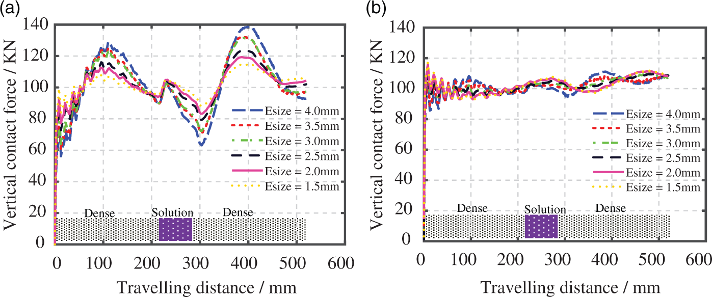$\lambda C_d$ .

To further evaluate the influence of mesh density at high level of contact stiffness, another six cases of varying mesh sizes are studied by increasing the penalty scale factor to the optimal one of $\alpha =12.8$ . Figure 11(b) shows the variation of the vertical contact forces with respect to different mesh sizes. The prior insistent statement that an increased penalty scale factor could eliminate the contact instability (“sudden perturbation”) has been further verified.

The reason for this phenomenon can be attributed to the reduced element size, which decreases from C_d to $\lambda C_d$ in the solution area (See Figure 12). Here, λ is a scale factor, $0<\lambda <1$ . Given a constant penetration depth l, it can be derived from equations (5) and (6) that

$$\lambda ·\lambda ·{\mathbf{f}}_s=-l·\alpha ·K·\lambda ·C_d·\mathbf{n}$$

(11)

From equations (5) and (11), it is found that the dal contact stiffness k contributed by the smaller elements ( $\lambda C_d$ ) only decreases by a factor of λ in comparison to that of large elements (C_d). But the overall contact stiffness (i.e. the summation of nodal contact stiffness $\sum k$ ) increases $\frac{1}{\lambda }$ times. For instance, if λ is $\frac{1}{4}$ , the overall contact stiffness will increase four times.

Figure 13(a) and (b) shows the variation of time step sizes with respect to different mesh sizes. With the decrease of the element size, both the contact and calculation time step sizes tend to drop.

Figure 13.

Variation of the time step sizes w.r.t. different mesh sizes: (a) default penalty scale factor α = 0.1; (b) optimal penalty scale factor α = 12.8.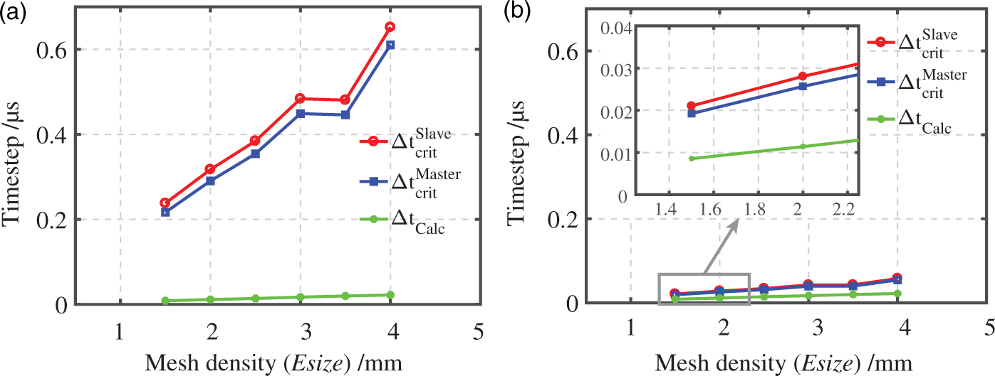

Figure 14(a) shows the normal contact pressure as a continuous contour plot for all the nodes in contact. It can be seen that the distribution of the normal contact pressure is getting converged towards the denser mesh, which also indicates that the denser the mesh is, the better the contact solution would be achieved.

Figure 14.

Effect of mesh size on contact pressure distribution: (a) nodal contour plot; (b) element contour plot.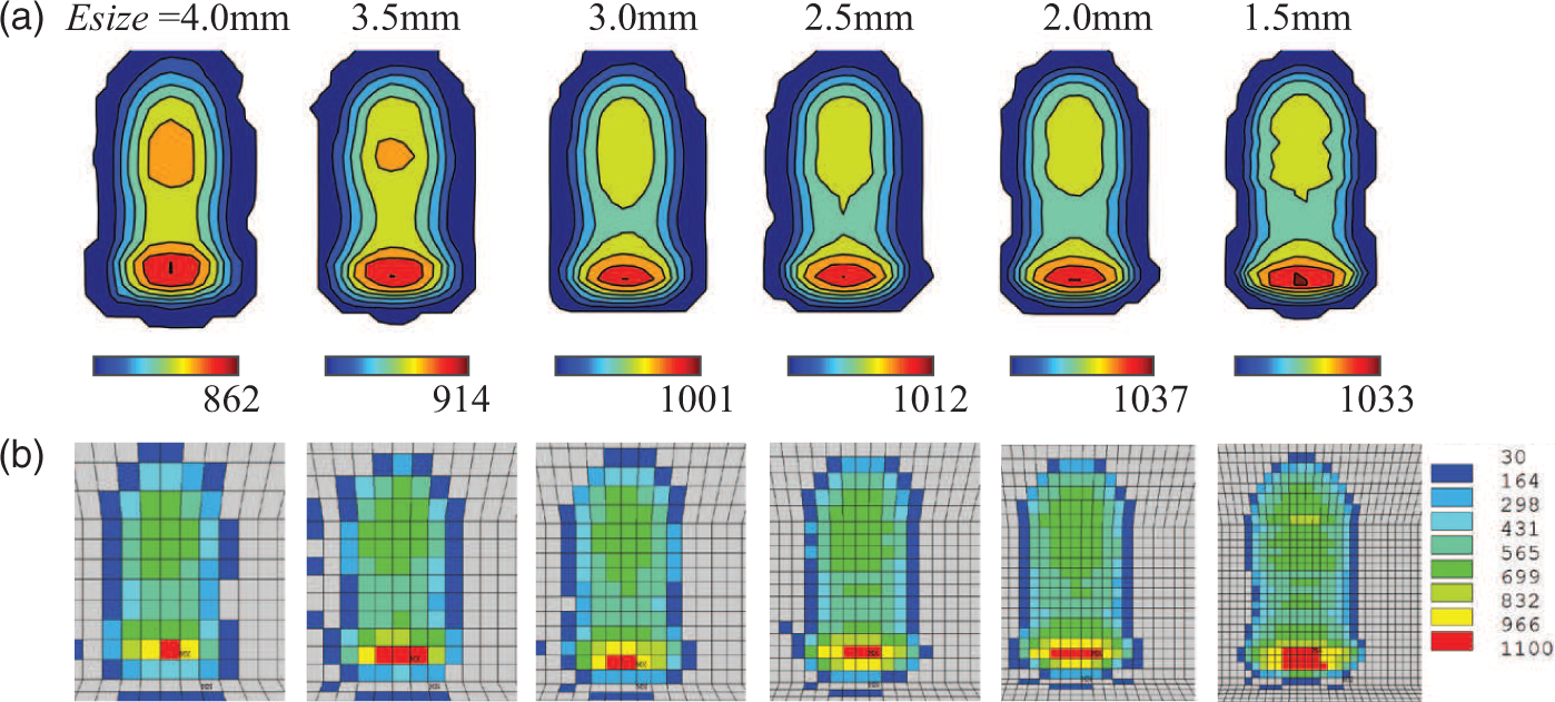

Figure 14(b) shows the normal contact solution results as discontinuous element contours. The discontinuity between contours of adjacent elements is an indicator of the stress gradient across elements. These element contours are determined by linear interpolation within each element, unaffected by surrounding elements (i.e. no nodal averaging is performed). Following the method presented in Ma et al., ³¹ the contact statuses of these elements are determined by the normal pressure σ_n as

$$\text{Anelementisincontact}:\mathit{if}{\sigma }_n>0$$

(12)

Table 2 lists the quantitative results in terms of the number of elements in contact and the size of the resulting contact patches. The maximum number of element in contact is 379 for the case of Esize = 1.5 mm, whereas it is only 73 for Esize = 4.0 mm. With the decrease of the mesh size Esize, the number of elements in contact increases significantly. Also, the size of the contact patch gets smaller in accordance with the mesh size.

Table 2.

Effect of mesh size on normal contact properties.

	Esize (mm)	Ac a (mm2)	N b	$A_c^{\mathit{mean}}$ c (mm2)
Case I	4.0	307.4	73	4.2
Case II	3.5	299.7	89	3.4
Case III	3.0	287.9	117	2.5
Case IV	2.5	277.0	154	1.8
Case V	2.0	265.8	218	1.2
Case VI	1.5	258.5	379	0.7

a

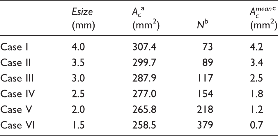
Real contact area.

b

Number of elements in contact.

c

Average contact area per element.

As the calculation expense would increase drastically due to the huge amount of elements generated, it is hardly possible to run the simulations with extremely small mesh size (e.g. 0.5 mm). The alternative is to run the simulation with a better selected parameter of mesh density, which could compromise between the calculation accuracy and efficiency in accordance with the criteria stated in the section of “Underlying challenges and possible solutions”. It is found that when the ratio of the contact area to the number of element in contact is around 1, a good compromise between calculation efficiency and accuracy is reached. Thus, the best mesh size at the dense meshed area is suggested to be 2.0 mm (Case V, see Table 2), while the one in the solution area is 1.0 mm. It is worth noting that the suggested mesh size in the solution area (i.e. 1.0 mm) falls within the range of 0.33 mm to 1.33 mm, which is recommended by Zhao and Li ¹⁹ to maintain an accuracy comparable to that of CONTACT and to satisfy the accuracy of engineering applications, respectively.

In summary, the mesh density can drastically influence the dynamic responses of W/R interaction when the contact stiffness is small. With the increase of the penalty stiffness, the dynamic response is getting less sensitive to the variation of mesh density. The denser the FE mesh is, the better the FE results can represent the reality.

Contact damping

Similar to the parametric cases studied previously, the contact damping factor VDC varies from 10 to 180. The corresponding dynamic responses of W/R contact forces are displayed in Figure 15. It can be seen that when the contact damping factor gets higher than 160, the resulting contact forces start to oscillate.

Figure 15.

Variation of the vertical contact forces w.r.t. different contact damping factors VDC: (a) default calculation time step 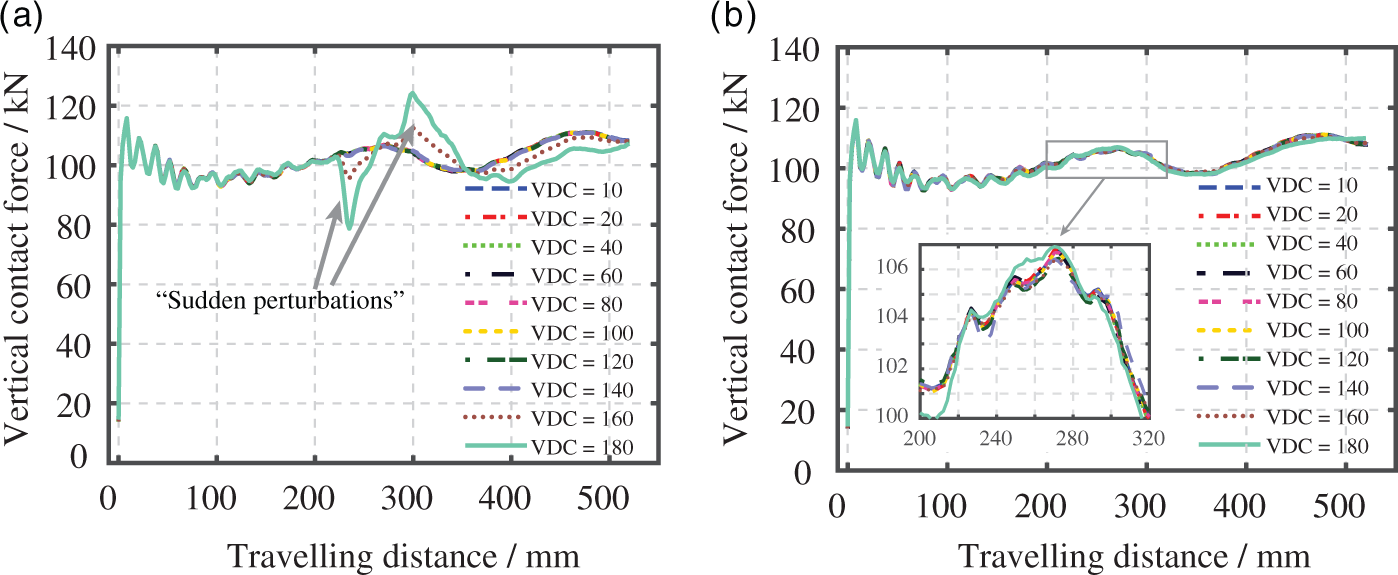$\Delta t_{\mathit{calc}}$ ; (b) reduced calculation time steps $\Delta t_{\mathit{calc}}$ .

According to equations (9) and (10), the “sudden perturbations” (nearby the solution area) are assumed to be caused by the fact that the value of the calculation time step size exceeds the magnitude of the reduced critical contact time step size. Attempts have been made to check the time step violations by comparing the contact time step sizes and the calculation time step sizes. It is found that the exported contact time step size only follows equation (8), which means that the influence of the contact damping as indicated by equation (9) is not considered for the output. As a consequence, all the contact time step sizes remain constant under different contact damping factors. Therefore, the check of time step violations such as the ones shown in Figures 9 and 13 are not presented in this section. But it is still assumed that the high contact damping is the main cause for the “sudden perturbations”.

To check the validity of the assumption, the calculation time step sizes $\Delta t_{\mathit{calc}}$ for the cases of VDC = 160 and VDC = 180 have been scaled down with two factors of 0.5 and 0.3, respectively. It is found that the variation of the vertical contact forces is getting stable again (see Figure 15(b)). This re-stabilization process of the contact forces implies that the contact damping would be another parameter, which can trigger the phenomenon of contact instability. The approach of retrieving the contact stability (if the phenomenon of contact instability happens) is to reduce the calculation time step size, but with the sacrifice of the calculation efficiency.

Figure 16 shows the variation of the contact pressure corresponding to different contact damping factors. It can be seen that both the magnitude and distribution of the contact pressure hold almost constant, which indicates that the influence of the contact damping factors on the contact pressure is insignificant. This agrees with the statement made by Hallquist ¹⁸ that contact damping tends to play an important role in the analysis of impact-related problems.

Figure 16.

Effect of contact damping on contact pressure distribution.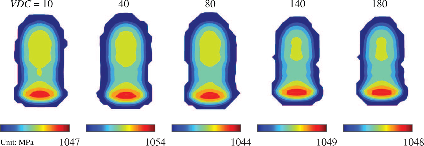

In short, the contact damping is a parameter that is less sensitive to the analyses of W/R interaction. The default damping factor VDC of 80 is good enough to fulfill the criteria of contact stability.

As reported in Tomberger et al., ³⁷ the sources of contact damping are relatively complex in reality, including the surface roughness, lubricant, liquid, etc. Although those over-critical damping factors (i.e. V DC > 100) employed may not have a direct physical correspondence, it is necessary to demonstrate the low sensitive effect of contact damping to the contact instabilities. Further investigation on the modeling of contact damping with high degree of realism is part of the future work.

Discussion: Applicability of suggested guidelines and parameters

From the parametric results, it can be recognized that the proposed guidelines are suitable for identifying an appropriate set of interface parameters. Those guidelines are not subjected to particular geometrical and/or technical restrictions (i.e. special contact geometries, hardware configurations, programming languages, etc.). Thus, it enables the suggested guidelines to have broad applicability in the area of explicit FE-based contact modeling, especially in which the contact constraints are enforced with penalty method. It is, also, recommended for further applications to other mechanical contact/impact systems (e.g., gear, bearing, etc.) that have complex local contact geometries.

With respect to the suggested interface parameters (i.e. penalty scale factor ( $\alpha =12.8$ ), damping factor (VDC = 80), mesh size (Esize = 2.0 mm), and uniformity (d₀ = 80 mm), it has reduced applicability in comparison to those guidelines. The reason is that the choice of interface parameters is strongly dependent on the level and form of the mesh discretization, which determine the magnitude of calculation and contact time step sizes and manifest themselves further in the phenomena of contact (in)stabilities.

In summary, the applicability of the interface parameters suggested is classified into two categories:

Suggested/similar mesh patterns as shown in Figure 1: The interface parameters suggested have wide applicability for the cases of different axle loads, train speeds, W/R profiles, etc. This can be explained by the recapitulated explicit FE theory, from which it finds that these varying operational patterns and geometrical parameters have no direct relations with the criteria of contact stability.

Taking the varying axle loads (ranging from 80 kN to 140 kN) as an example (see Figure 17), the interface parameters suggested are capable of suppressing the oscillations of contact forces, and thus maintain the contact stability effectively. Also, with the increase of the axle load, a steady growth of the area of contact patches and the magnitude of contact pressure is observed.

Figure 17.

Applicability of interface parameters suggested to the cases of varying axle loads: (a) vertical contact forces; (b) contact pressure.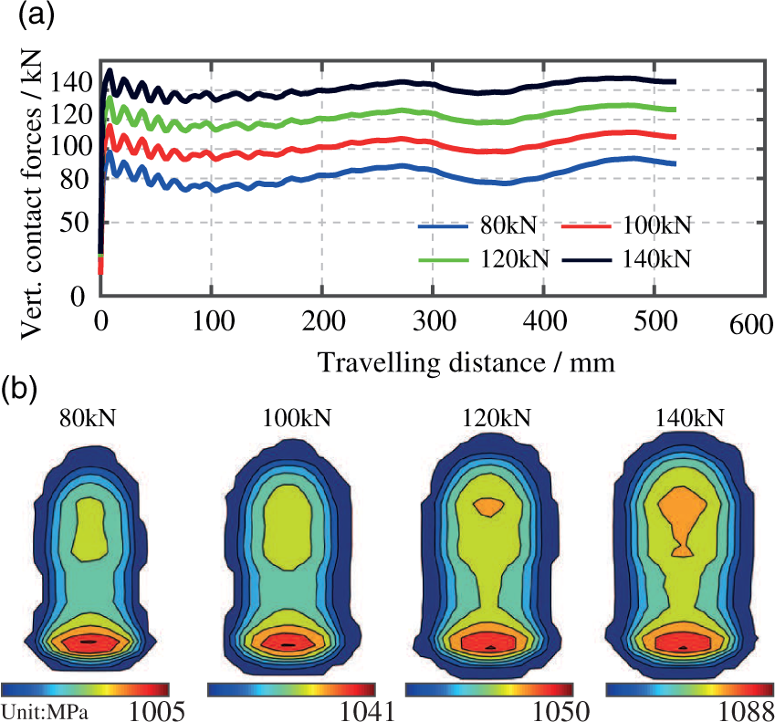

It has also been demonstrated in Ma et al.^31,32 that the interface parameters suggested are suitable for the cases of varying operational patterns (i.e. varying friction and traction) and contact geometries (e.g. crossing rail).

Different mesh patterns: When the form (uniformity) and level (density) of mesh discretization change, the magnitudes of both the calculation $\Delta t_{\mathit{calc}}$ and contact $\Delta t_{\mathit{cont}}^{\mathit{slave}(\mathit{master})}$ time step sizes will be affected (see Figures 9 and 13). Thus, the suitable interface parameters that are determined based on equation (10) might differ from those suggested. In other words, the interface parameters suggested need to be improved to fit the changing mesh pattern.

Taking the selection of good penalty scale factor α_optimal as an example, Figure 18(a) schematically shows the relation (i.e. adapted from Figure 4(b)) between the calculation and contact time step sizes. As discussed previously, the optimal penalty scale factor α_optimal is selected at the vicinity of the unstable area (i.e. $\Delta t_{\mathit{calc}}>\Delta t_{\mathit{cont}}^{\mathit{slave}(\mathit{master})}$ ).

Figure 18.

Effect of mesh patterns on the selection of optimal penalty scale factor α: (a) reference case (generalized from Figure 4(b)); (b) variation of 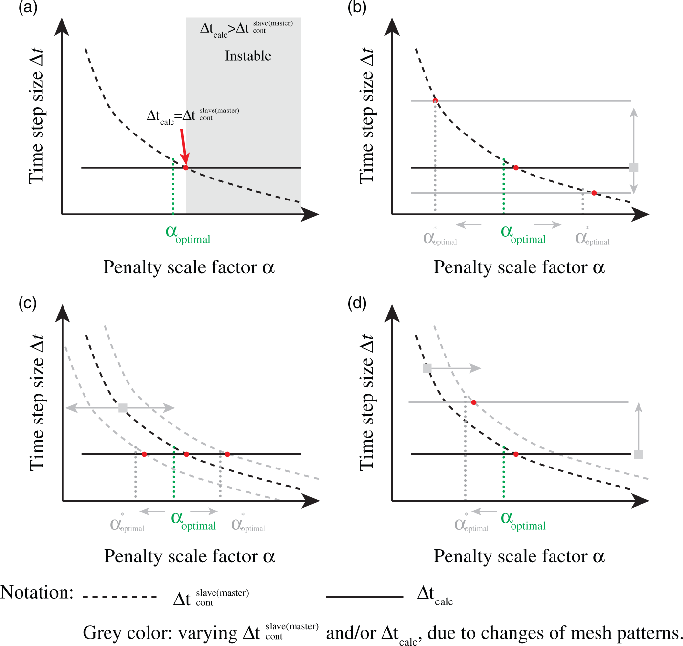$\Delta t_{\mathit{calc}}$ ; (c) variation of $\Delta t_{\mathit{cont}}^{\mathit{slave}(\mathit{master})}$ ; (d) variation of $\Delta t_{\mathit{calc}}$ and $\Delta t_{\mathit{cont}}^{\mathit{slave}(\mathit{master})}$ .

For this reason, the change in the optimal penalty scale factor, alongside the varying mesh patterns, is divided into three groups:

Variation of $\Delta t_{\mathit{calc}}$ (see Figure 18(b)): If the minimum side length of solid element varies, the curve of calculation time step size $\Delta t_{\mathit{calc}}$ moves up and down. Accordingly, the optimal penalty scale factors α_optimal selected have to shift.

Variation of $\Delta t_{\mathit{cont}}^{\mathit{slave}(\mathit{master})}$ (see Figure 18(c)): If the mesh size of contact elements varies, the curves of contact time step $\Delta t_{\mathit{cont}}^{\mathit{slave}(\mathit{master})}$ will offset laterally. This is complementary to the variation of the contact time steps shown in Figure 9. Similarly, the optimal penalty scale factors selected will change.

Variation of both $\Delta t_{\mathit{calc}}$ and $\Delta t_{\mathit{cont}}^{\mathit{slave}(\mathit{master})}$ (see Figure 18(d)): In this case, the optimal penalty scale factors will move both horizontally and vertically.

In summary, when the mesh patterns are significantly different from that shown in Figure 1, it is suggested to follow the general guidelines to find the suitable interface parameters.

Conclusions and outlook

In this paper, the effect of W/R interface parameters on the contact stability in the explicit FE analysis has been studied. The numerical phenomena called “contact (in)stabilities” have been presented.

Based on the results of this study, it is concluded that the interface parameters (e.g. contact stiffness, damping, mesh size, etc.) strongly affect the accuracy of contact solutions and must be selected carefully. The wrong choice of these parameters (such as too high/low contact stiffness and damping, course mesh, or wrong combination of these parameters) can result in an inaccurate solution of the contact problem that manifests itself in the amplification of the contact force or/and inaccurate contact responses (mainly due to the contact instability). The choice of these parameters used in the explicit FE analysis has to be justified.

The guideline for the selection of optimum interface parameters, which guarantees the contact stability and therefore provides an accurate solution, is proposed. According to this guideline, the time steps in the explicit analysis $\Delta t_{\mathit{calc}}$ and $\Delta t_{\mathit{cont}}^{\mathit{slave}(\mathit{master})}$ , which are determined by the interface parameters, must be tuned as close as possible to each other.

An appropriate set of interface parameters is suggested (i.e. penalty scale factor (12.8), damping factor (80), mesh size (dense meshed area: 2.0 mm; solution area: 1.0 mm) and uniformity (80 mm)). In comparison with the general applicability of the proposed guidelines (e.g. other mechanical contact/impact systems), the interface parameters suggested have reduced applicability.

Further research on the contact instabilities excited physically by friction or surface defects (i.e. wheel-flats, corrugation, squats, etc.) is part of the future work.