Sage Journals: Discover world-class research

Abstract

Over the past few years, a number of implicit/explicit finite element models have been introduced for the purpose of tackling the problems of wheel–rail interaction. Yet, most of those finite element models encounter common numerical difficulties. For instance, initial gaps/penetrations between two contact bodies, which easily occur when realistic wheel–rail profiles are accounted for, would trigger the problems of divergence in implicit finite element simulations. Also, redundant, insufficient or mismatched mesh refinements in the vicinity of areas in contact can lead to either prohibitive calculation expenses or inaccurate implicit/explicit finite element solutions. To address the abovementioned problems and to improve the performance of finite element simulations, a novel modelling strategy has been proposed. In this strategy, the three-dimensional explicit finite element analysis is seamlessly coupled with the two-dimensional geometrical contact analysis. The contact properties in the three-dimensional finite element analyses, such as the initial “Just-in-contact” point, the exact wheel local rolling radius, etc., which are usually a priori unknown, are determined using the two-dimensional geometrical contact model. As part of the coupling strategy, a technique has been developed for adaptive mesh refinement. The mesh and mesh density of wheel–rail finite element models change adaptively depending on the exact location of the contact areas and the local geometry of contact bodies. By this means, a good balance between the calculation efficiency and accuracy can be achieved. Last, but not least, the advantage of the coupling strategy has been demonstrated in studies on the relationship between the initial slips and the steady frictional rolling state. Finally, the results of the simulations are presented and discussed.

Keywords

Improving performance finite element analysis wheel–rail interaction coupling strategy geometrical contact analysis

Introduction

Rolling frictional contact between wheel and rail (W/R) is a highly non-linear problem involving large deformation, large rotation, material plasticity, contact, friction, etc. With the development of modern computing techniques and the availability of supercomputers, advances in the field of numerical simulations on such complex problems have been strongly boosted. Among the various numerical methods proposed,^1–4 the finite element (FE) method is more widely used, by virtue of its striking versatility (i.e. accounting for arbitrary contact geometries, material plasticity, etc.). In general, based on the different features of solution procedures, the FE methods are classified into two main categorises,^5,6 namely implicit and explicit.

Regarding the implicit FE method, a variety of models/tools have been created for different engineering purposes.^7–12 For instance, Wiest et al.⁷ performed implicit FE analyses to predict the normal pressure of W/R impact at a crossing nose. Telliskivi et al.¹¹ developed an implicit FE model to understand the complex behaviour of W/R interaction. The ratcheting performance of rail steels was evaluated by Pun et al.⁸ The problem of normal contact was resolved using a quasi-static FE simulation, while the tangential shear stress distributions were calculated according to Carter’s theory.⁴ The effect of wheel motions on the distribution of residual stresses was studied by Bijak-Żochowski and Marek.¹⁰ Mandal and Dhanasekar⁹ presented a novel sub-modelling approach to investigate the ratcheting failure of insulated rail joints. Based on the detailed stress/strain responses obtained from FE simulations, attempts were made by Ringsberg et al.¹² to predict the fatigue life of crack initiation on the rail surface. Ma et al.¹³ introduced an implicit FE tool to qualitatively evaluate the performance of different rail pre-grinding strategies. However, due to the difficulties of convergence and the absence of dynamic effects,^5,6 these implicit FE approaches were no longer able to meet the increasing expectations of FE-based contact models possessing higher degree of realism and better accuracy.

As an alternative problem-solving procedure (i.e. opposed to the implicit FE method), the explicit FE simulation proceeds without solving a large set of simultaneous equations at each time step and inverting the large matrix.^5,6,14,15 This enables the explicit FE method to avoid certain difficulties of non-linear programming that the implicit method usually has.¹⁶ Owing to such intrinsic advantages, the explicit FE approach is being increasingly welcomed for combatting the associated problems of W/R interaction. More recently, a series of representative three-dimensional (3D) explicit FE models^17–20 have been presented. Zhao and Li¹⁷ developed a 3D explicit FE model for W/R interaction. The model was successfully verified against CONTACT. An explicit FE tool was created to simulate the W/R contact–impact at rail insulated joint by Wen et al.²⁰ It was found that the variation of axle load had stronger effects on the impact event than other operational parameters. Pletz et al.¹⁹ presented a dynamic wheel/crossing FE model to investigate the influence of operational parameters, such as axle loads, train speeds, material properties, etc., on the impact phenomena. The stress states and material responses under different levels of adhesions were analysed by Vo et al.¹⁸ It was anticipated that the rail was highly prone to the damage resulting from the ratcheting fatigue of the material.

In summary, significant progress in the field of FE simulations on W/R interaction, from which a number of valuable insights are gained, has been made. Yet, there is still much work to be done. For example, the “gaps or penetrations” between wheel and rail interfaces cause the problems of divergence in the implicit analyses^15,16 or even an unexpected failure in the explicit FE analyses.²¹ Also, due to a priori unknown contact location, the general experience- or visualisation-based discretisation on the potential contact area could always lead to a redundant, insufficient or mismatched FE mesh. As a consequence, the efficiency and accuracy of FE simulations would be adversely affected.

To address these modelling challenges (explained later in detail) and to improve the performance of FE simulations, a new coupling strategy, that couples the two-dimensional geometrical (2D-Geo) contact analysis and the three-dimensional explicit finite element analysis, has been proposed. The idea of this strategy is inspired by the approach used in CONTACT (i.e. a well-established computational programme developed by Professor Kalker²² and powered by VORtech Computing³). Prior to the 3D-FE analysis, the 2D-Geo contact analysis is functioning effectively as an adaptive guidance for the identification and discretisation of the potential area in contact. The challenge of the coupling strategy lies in the programming efforts on how to build up the 2D-Geo and 3D-FE models as well as how to make the interface of two models work effectively. Based on the simulation results, it has been noticed that the computational problems, such as gaps/penetrations, mesh refinement, unexpected initial slips, etc., have been resolved successfully. The goal of improving the performance of FE simulations has thus been achieved with the aid of this coupling strategy.

The outline of this paper is as follows. In the next section, full attention is focused on the general descriptions of the 3D-FE model. Also, the details of FE modelling challenges, that prohibit the analysts from attaining accurate contact solutions, are presented. The strategy (referred to as ‘enhanced explicit FE-based coupling strategy’, abbreviated as ‘eFE-CS’, hereinafter), which couples the 2D-Geo model together with that of 3D-FE, is described in the Coupling strategy section. Following that, the effectiveness and advantages of ‘eFE-CS’ strategy are demonstrated in the FE results and discussion section. Finally, concluding remarks are drawn.

W/R 3D-FE model

In this section, the FE model for the analysis of W/R interaction is presented. The two counterparts investigated here are the standard S1002 wheel²³ (EN13715-S1002/h28/e32.5/6.7%) with a nominal rolling radius of 460 mm and the standard UIC 54E1 rail. Here, ‘h28’ refers to the flange height of 28 mm; ‘e32.5’ means the flange thickness of 32.5 mm; ‘6.7%’ is the reverse slope. The drawing of wheel cross section is adopted from International Union of Railways.²⁴ The inner gauge of the wheel-set is 1360 mm and the axle length is 2200 mm. The track gauge is 1435 mm. Also, the cant angle of 1/40 is considered in the model. Note that the model can be easily adjusted to account for other different W/R profiles.

Discretised FE model

A half W/R FE model shown in Figure 1(a) and (b), where the rail is modelled with restriction to an overall length of 1.8 m, is adopted by taking advantage of the symmetrical characteristic of the track and the wheel-set. Such a half W/R FE model is similar with and inspired by the ones described in the literature.^19,20 The wheel is set to roll from the origin of the global coordinate system O–XYZ over a short travelling distance d on the rail (see Figure 1(a)). The global coordinate system is defined as: the X-axis is parallel to the longitudinal direction along which the wheel-set travels, the Z-axis is the vertical pointing upwards and the Y-axis is perpendicular to both the X and Z directions, forming a right-handed Cartesian coordinate system.

Figure 1.

FE model of the W/R interaction: (a) schematic graph and (b) front view.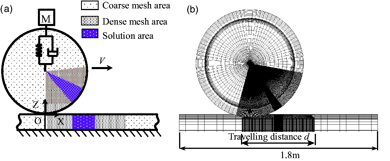

Only the regions where the wheel travels are discretised with dense mesh, leaving the remaining regions with coarse mesh (see Figure 1(a) and (b)). A solution area is introduced and positioned in the middle of the dense meshed area. Here, the solution area is defined as a region to extract and analyse the contact properties, such as the contact patch, normal pressure, shear stress, etc. In this region, the mesh size (1 mm) is approximately two times smaller than the dense meshed area (2 mm) for the purpose of capturing the associated high stress/strain gradients.

To take the primary suspension into account, a group of sprung mass blocks are lumped over the spring–damper system. Figure 7(b) shows the eight spring–dampers created, which attempt to avoid the high stress concentrations on the elements of wheel axle centre. The errors of negative volumes can thus be minimised/eliminated, which will facilitate the success of explicit FE simulations. The mass blocks that represent the weight of the loaded car body are 10 tons. The corresponding parameters of the springs and dampers are listed in Table 1. Linear elastic material model is used to describe the constitutive relation of W/R components.

Table 1.

Material properties and mechanical parameters.

	Properties	Values
Wheel/rail material^a	Young’s modulus (GPa)	210
Wheel/rail material^a	Poisson’s ratio	0.3
	Density (kg/m³)	7900
Primary suspension	Stiffness (MN/m)	1.15
Primary suspension	Damping (Ns/m)	2500
Operational parameters	Friction coefficient	0.5
Operational parameters	Traction coefficient	0.25
	Train velocities (km/h)	140
	Lateral displacement (mm)	0.0

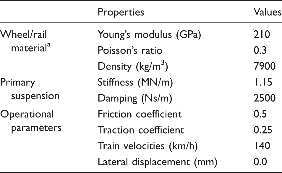
Note: “a”: Linear elastic material.

To better simulate the process of W/R dynamic contact, an implicit-to-explicit sequential solving procedure²¹ is adopted. In this procedure, the implicit solver (ANSYS Mechanical¹⁵) and explicit solver (ANSYS LS-DYNA²¹) work in pairs. First, the equilibrium state of the preloaded structure (e.g., under the axle-load of 100 kN) is determined with ANSYS Mechanical. The displacement results of the implicit analysis are used to do a stress initialisation for the subsequent transient analysis. Then, the processes of rolling frictional contact begin at time zero with a stable preloaded structure.¹⁵ The responses of dynamic contact are further simulated with ANSYS LS-DYNA following the scheme of central difference time integration.²¹

For such a typical FE analysis of dynamic contact, the basic process consists of three tasks: (1) Build the model, including prescribing the initial location of W/R, defining correct boundary conditions, preforming mesh refinement, etc. (2) Apply the loads and run the simulations, involving traction application, contact definition and determination of calculation time step size; (3) Review the results, referring to the visualisation of contact properties, such as surface normal pressure, shear stresses within the actual contact patches, subsurface stress/strain responses, etc.

Challenges of FE analysis

As the contact always occurs at a priori unknown area, a series of obstacles will thus be encountered when performing FE-based contact simulations. In this section, the details of those obstacles are presented and discussed.

Geometrical gaps/penetrations

Figure 2 shows the ‘gaps/penetrations’ between the contacting bodies of W/R. Both the gaps and penetrations are undesired. For example, in the implicit FE analyses, too large gap may lead to the wrong identification of contact pairs, while prominent penetrations may cause the overestimation of contact forces. Consequently, it causes an unexpected failure (usually the error of divergence) of the FE simulation. For explicit FE analyses, no penetrations are allowed and the gaps can increase the calculation cost significantly for eliminating the effect of initial disturbances.

Figure 2.

Schematic of initial contact status: (a) penetration, (b) gap and (c) just-in-contact.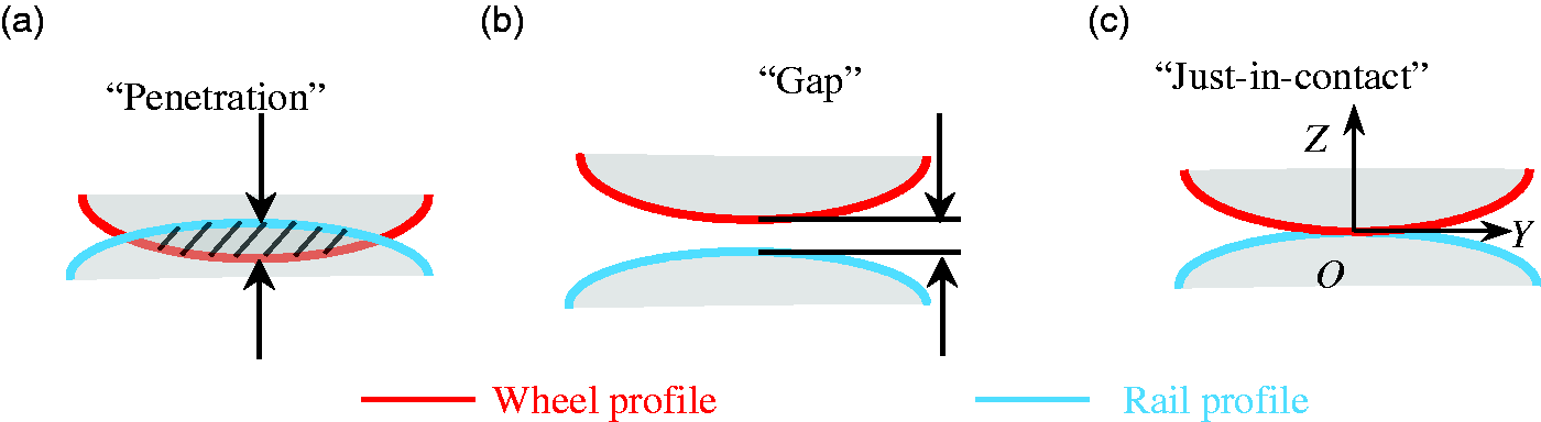

Although there are several options (i.e. tuning the real constants and key options of contact elements independently or in combination) suggested in ANSYS to adjust the initial contact conditions, they do not work well when the values of gaps/penetrations are large (e.g. in the order of millimetres or even larger). Also, it is quite challenging to manually bring the two W/R contacting bodies into the positions of “Just-in-contact” as shown in Figure 2(c). Here the term of “Just-in-contact” refers to a contact positioning between wheel and rail, where the two bodies touch each other without or with a tolerable contact gap or penetration. Moreover, due to the complexity of W/R realistic contact geometry, it is very difficult to determine where the first point of contact will occur. Thus, the gaps/penetrations appear to be inevitable and troubling.

Preload application

As shown in Figure 3, the wheel is prescribed to travel over the rail from the initial condition of pure rolling state to the steady state of partial slip. Here, the steady state²² means that the slip-adhesion phenomenon is independent of time. To achieve the initial state of pure rolling without slip, the velocity V_CP of the contact point CP should be zero. The initial translational velocity V₀ and the initial angular velocity ω₀ are thus related by

V_{0} = R_{w} ω_{0}

(1)

Figure 3.

Schematic of the wheel kinematics (note: “C” denotes the wheel centre-of-mass).

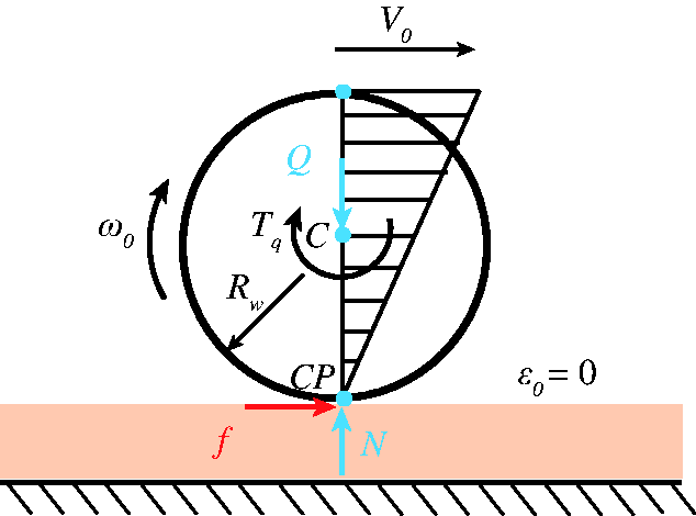
As the “Just-in-contact” point is a priori unknown, the real local wheel rolling radius R_w at the point of contact CP would be difficult to predict. In case if it is wrongly predicted as $R_{w}^{*}$ , the initial angular velocity will be derived as $ω_{0}^{*} = V_{0} / R_{w}^{*}$ and then improperly applied on the wheel. Thus, an unexpected initial slip ɛ₀, which is defined as²⁵

ɛ_{0} = (V_{0} - ω_{0}^{*} R_{w}) / V_{0} = (1 - R_{w} / R_{w}^{*}) \neq 0

(2) will be introduced and exerted onto the system of W/R dynamic contact.

In addition, to reproduce the local phenomenon of partial slip numerically, the appropriate traction torque T_q is derived from the viewpoint of classical mechanics²⁶

T_{q} = \frac{J_{c} + {mR}_{w}^{2}}{{mR}_{w}} f

(3) where f is the frictional force, m represents the mass of the wheel and J_c is the moment of the inertia of the wheel. It is obvious that any wrong estimation of the local wheel radius R_w may lead to the inaccurate application of the traction T_q.

Mesh refinement

Given that the refined element size inside the contact patch should be as small as 1000 times over the dimension of W/R components, an economic, adaptive and reliable mesh generation has always been a challenge for the analysts.

However, there are no clear rules proposed for determining the size of the refined potential contact area up to now. The most commonly adopted approach is the trial-and-error method mainly depending on the researchers’ experience or visualisation. Using this method, the refined potential contact area can be easily overestimated or underestimated (see Figure 4(a) and (b)). In particular cases, the refined potential contact areas might be mismatched or deviated from each other (see Figure 4(c)). Thus, the trial-and-error method is highly prone to the inaccurate or undesired contact solutions of W/R interaction.

Figure 4.

Schematic of the mesh refinement at the potential contact area: (a) Redundant, (b) Insufficient, (c) Mismatched and (d) Idea.

In addition, if the relative contact locations between the wheel and the rail vary along the track, the corresponding mesh refinement is in demand to be altered spontaneously. This brings about an even higher requirement on the flexibility of the mesh refinement approach.

Coupling strategy

To deal with the aforementioned challenges of FE analyses, a novel coupling strategy, that combines 2D-Geo contact analysis and 3D-FE analysis, is developed (see Figure 5). The purpose of the 2D-Geo simulation is to detect and determine the initial “Just-in-contact” location (CP), the contact clearance and the corresponding local wheel rolling radius at the point of contact. The obtained contact information is used as the adaptive guidance for the 3D-FE analysis (see W/R 3D-FE model section).

Figure 5.

Working mechanism of the coupling strategy.

To implement this coupling strategy, the data exchange between 2D-Geo and 3D-FE models is performed by a small external routine written in the MATLAB environment. Once the processes of 3D-FE modelling and preloading are accomplished, the dynamic simulation is performed to study the behaviour of W/R contact. The details of the 2D-Geo analysis and the interfacing scheme of the two models are briefly described in this section.

2D-Geo analysis

In order to better illustrate the 2D-Geo contact model, a rigid wheel-set is positioned over a rigid track shown in Figure 6(a). The global coordinate system O–XYZ is complementary to the one shown in Figure 1. $O^{t} - X^{t} Y^{t} Z^{t}$ and $O^{w} - X^{w} Y^{w} Z^{w}$ refer to the wheel-set- and track-based coordinate systems, respectively. Since the model is 2D, only the roll motion θ and the lateral shifts δy of a wheel-set as shown in Figure 6(a) are considered.

Figure 6.

(a) W/R 3D coordinate systems and (b) “Just-in-contact” equilibrium condition of the wheel–rail at a lateral displacement of −10 mm.

Figure 7.

(a) “Just-in-contact” equilibrium location derived from the 2D-Geo contact analysis and (b) the cross sectional view of the W/R dynamic contact FE model.

The current 2D-Geo contact model is further developed on the basis of the previous work.¹³ The initial contact points, where the two particles on the un-deformed wheel and rail coincide with each other, are determined under a given lateral displacement of the wheel-set. The solution procedure of 2D-Geo model is non-iterative by taking advantage of efficient matrix operations in MATLAB, which means that no inner and/or outer loop iterations (e.g. ‘for’ or ‘while’ loops) of exploring the “Just-in-contact” equilibrium conditions are performed. By this means, a significant increase in the calculation efficiency (around 10 s) is accomplished, as opposed to the conventional iterative fashion (e.g. 2–3 min in Ma et al.¹³). More information about the contact searching schemes is given in the literature.^13,27,28 Figure 6(b) shows a typical example of the 2D-Geo contact analysis, in which the wheel-set is located at the “Just-in-contact” equilibrium position with a lateral displacement of −10 mm.

Coupled interface

Using the 2D-Geo model described above, the interface and outcome of the ‘eFE-CS’ strategy are presented below.

“Zero” gaps/penetrations and obtained R_w

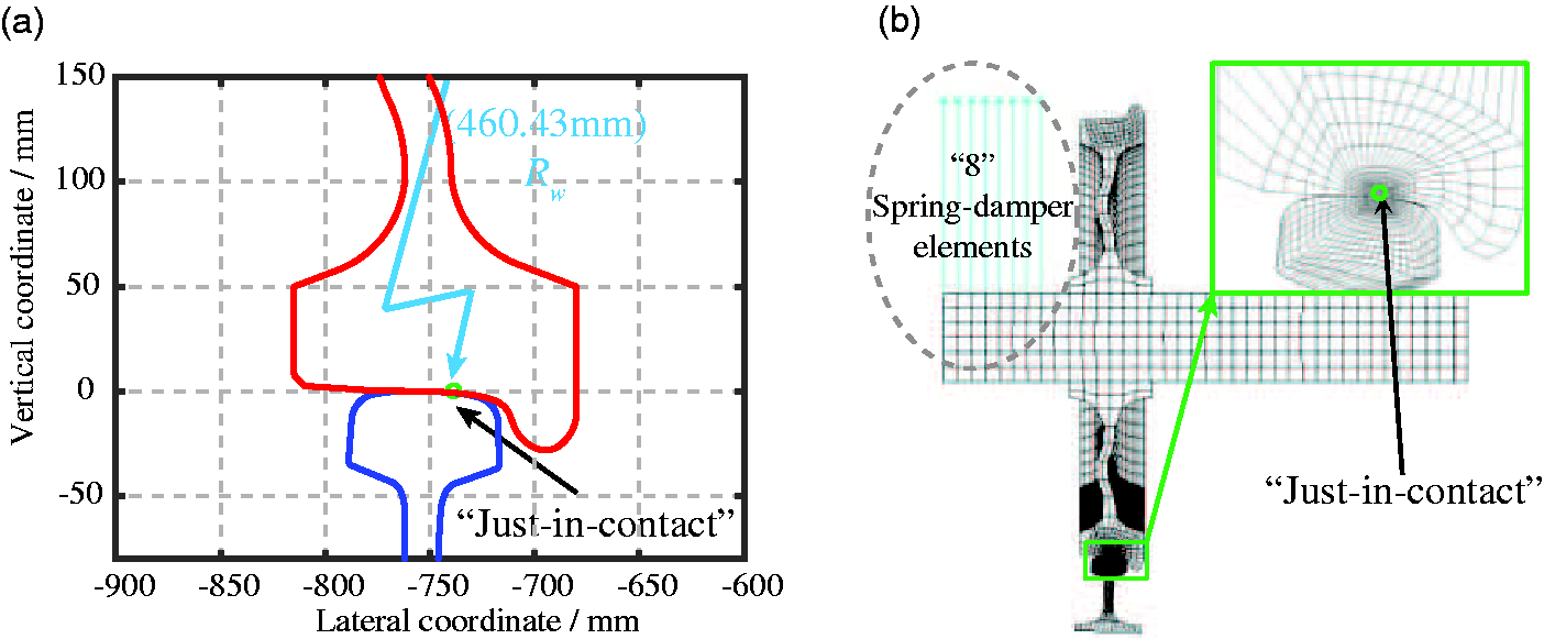
Figure 7(a) shows the results of the 2D-Geo contact analysis, through which the 2D wheel-set is positioned on the “Just-in-contact” point of the track. Depending on the lateral displacement and roll angle of the wheel-set determined by the 2D-Geo analysis, the wheel position in the 3D W/R FE model (see Figure 7(b)) has been properly adjusted. The resulting gaps or penetrations between wheel and rail can be reduced to the order of a micrometre or even less. This ensures a successful FE simulation of W/R interaction by taking advantage of the suggested options in ANSYS (see Geometrical gaps/penetrations section).

Besides, the actual rolling radius R_w corresponding to the given lateral displacements of the wheel-set can be obtained. For example, at the lateral shift of 0 mm, the exact local wheel rolling radius R_w is 460.43 mm, which is denoted by a cyan arrow as shown in Figure 7(a).

New adaptive mesh refinement

Considering that the refined potential contact area should completely encompass the actual contact area^3,22 (see Figure 8(b)), the calculated contact clearance from 2D-Geo analysis is used as the adaptive guideline for the mesh refinement of W/R interface. Here, the term of “Contact clearance” δz (see Figure 8(a)) is defined by the vertical distance between the wheel and rail for the un-deformed contact geometry. The value of the contact clearance defines the region with high susceptibility for contact to occur (also called the potential contact area). It is assumed that the most stressed point inside the contact patch coincides with the initial contact point (‘CP’ in Figure 8(a)). The origin of the mesh refinement is designated to the initial CP. The width of the refined region Δy is gradually arising with the increase of the contact clearance (see Figure 8(c) and (d)).

Figure 8.

Schematic representation of the new adaptive refining approach: (a) global view of contact clearance; (b) schematic graph of the potential and actual contact areas; (c) close-up view on the variation of contact clearance at the vicinity of initial contact points and (d) close-up view of the refined potential contact region.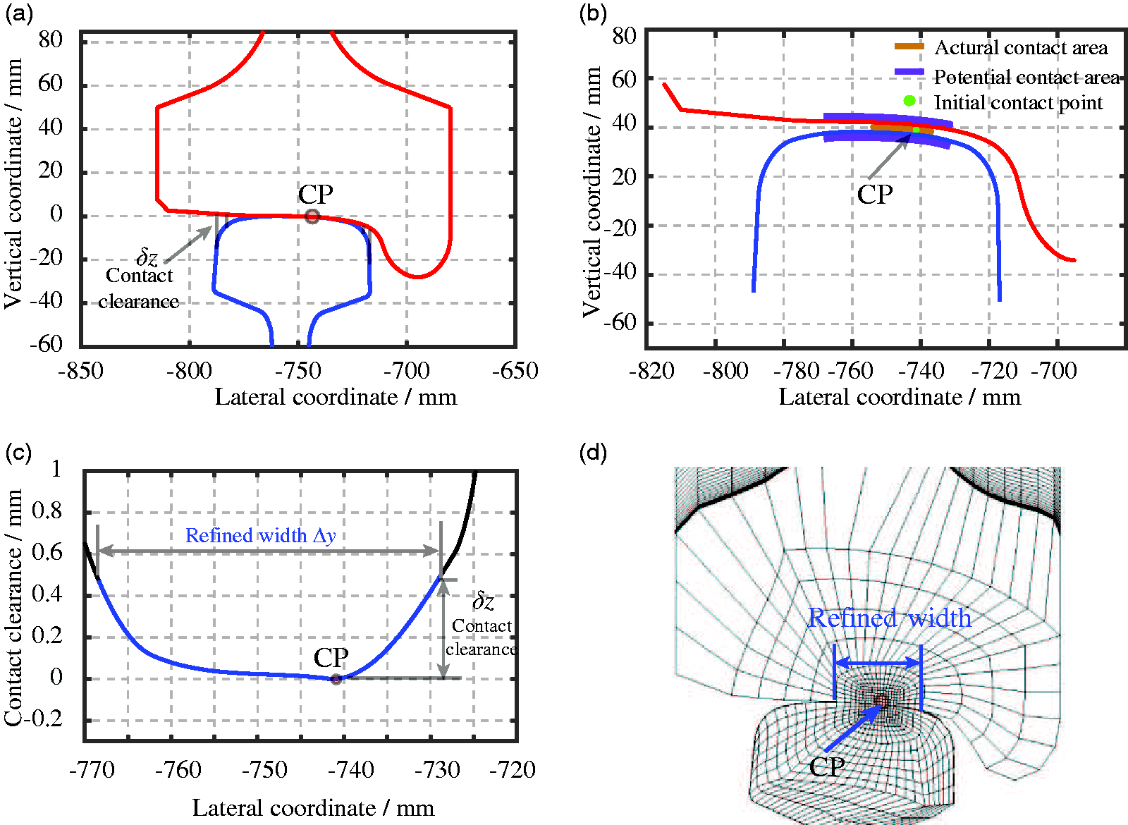

For the sake of identifying the best contact clearance, it is expected to follow a guideline as follows:

The contact clearance δz should be small enough to constrain the size of the model and thus maintain the calculation expenses into a low level.

The refined potential contact area determined by the contact clearance δz should be sufficient to encompass the resulting real contact patch obtained from the FE analysis.

Based on the selected value of the contact clearance, the mesh refinement process in these regions will be initiated. Using the proposed Nested Transition Mapped mesh refining approach,²⁹ the elements in the solution area are able to be refined as small as 1.0 mm × 1.0 mm × 1.0 mm (as shown in Figures 8(d) and 10), while for the remaining out-of-contact region (coarse mesh area), less attentions will be paid.

Figure 9.

Flexibility of the new mesh refining approach with respect to. different lateral displacements: (a) 5.5 mm; (b) 2.0 mm; (c) −3.5 mm and (d) −5.5 mm.

Figure 10.

The resulting contact pair: (a) isometric view and (b) side view.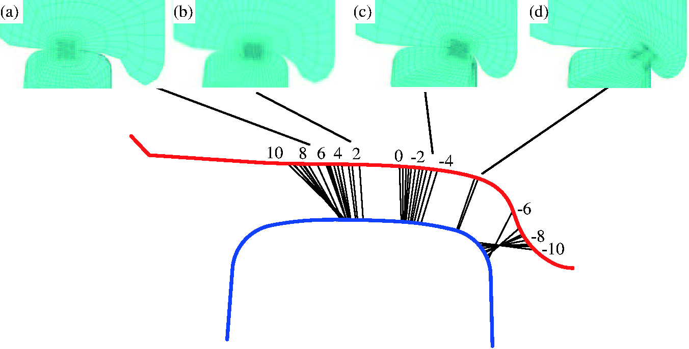

Flexibility of the new mesh refining approach

To automate the common tasks and implement the coupling strategy more efficiently, both the 2D-Geo and 3D-FE models have been coupled and parametrised using the scripting language of MATLAB and Parametric Design Language of ANSYS (APDL). The scripted and later packaged ‘eFE-CS’ modelling strategy offers great convenience and flexibility for the day-to-day analyses.

One added important feature of this adaptive mesh refining method is shown in Figure 9, where the patterns of these local mesh refinements change flexibly with respect to different lateral displacements of the wheel-set (e.g. ranging from −5.5 mm to 5.5 mm). For the cases of non-zero lateral displacements, the rails remain symmetric in relation to the track centre, while only the wheel and contact conditions vary. The variations of geometrical contact properties associated (i.e. locations and dimensions of refined potential contact areas) are predicted by a priori 2D-Geo contact analysis (see Figure 6(b)). Once the FE models (i.e. with half W/R considered) are created, they are used to study the dynamic behaviour of W/R interaction. Here, the applicability of this half W/R FE modelling approach (as shown in Figure 1) to the cases of different lateral displacements are explained as:

A complete wheel-set and two rails are considered in the 2D-Geo contact model (see Figure 6). The roll angles of the wheel resulting from the variation of lateral displacements have been explicitly taken into account.

A range of lateral displacements (i.e. (−5.5 −5.5) mm) cover most sections of railway track (e.g. tangent, large radius curves, etc.),³⁰ where the yaw angles (also called attack angle) are usually small (less than 2°³¹). Moreover, being aware that the wheel travels over a relatively short distance of 0.52 m, which is rather short in comparison to the wavelength of yaw/Klingel motion (i.e. usually in the order of 10–100 m), the variation of yaw angle would be relatively small. It is thus assumed that the neglect of yaw motion in the model presented might be acceptable.

A comprehensive model verification against CONTACT³ has been performed by the authors recently.³² For the cases of different lateral displacements (i.e. (−5.5 −5.5) mm), the model verification shows that the half W/R FE model can produce as good results as CONTACT.

In summary, the half W/R FE model enhanced with 2D-Geo contact analysis is flexible enough to be used in the cases of different lateral displacements. However, the further applicability of half W/R FE model to the sharp curves (i.e. curve radius smaller than 500 m³³), in which the yaw angle is indispensable and plays an important role, will be explained later in the Discussion: Pros and cons of ‘eFE-CS’ model section.

Resulting contact pairs

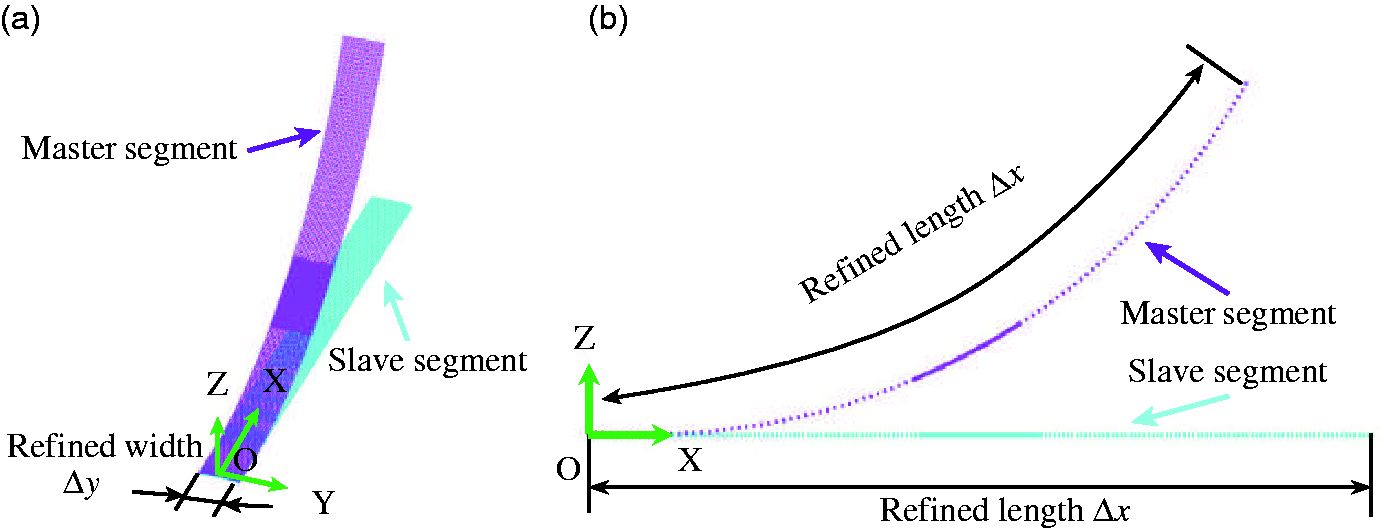
Figure 10(a) and (b) shows a contact pair, consisting of two master and slave segments for explicit FE analysis (TARGET 170 and CONTACT 173 elements for implicit FE analysis). It can be seen that the size of the potential contact area is controlled by the magnitude of the refined width Δy in the lateral direction (see Figure 8) and the refined length $Δ x$ in the longitudinal direction (see Figure 1). Here, potential contact areas are defined by the two curved rectangles on the outer layers of the W/R interfaces.

It has been reported in the literature^34,21 that contact analysis will add a significant computational cost for the overall solution, even when the ratio between the number of contact points and the number of elements is small. To limit the level of calculation expense as low as possible, the smallest and localised contacting zones are always desired to maintain the most efficient solution. Also, as discussed before, the refined potential contact areas should be large enough to encompass all the necessary contacts to maintain the accuracy of the solution. According to the coupling strategy, the refined width Δy is defined in the 2D-Geo analysis in terms of the contact clearance δz, while the refined length $Δ x$ is defined in terms of the travelling distance d. In the following section, the effects of corresponding geometrical parameters on the performance of FE simulations are studied.

FE results and discussion

To demonstrate the effectiveness of the ‘eFE-CS’ strategy, a series of FE simulations have been performed. The influence of the size of potential contact areas and the local wheel rolling radius on the performance of ‘eFE-CS’ strategy are to be analysed. As the wrongly estimated rolling radius $R_{w}^{*}$ will result in an initial slip ɛ₀ (see equation (2)), the investigation on the effect of local wheel rolling radius R_w is replaced here by the initial slip ɛ₀.

Contact clearance

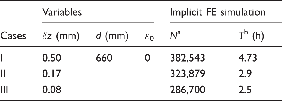
Figure 11 shows the effect of contact clearances (δz) on the FE models. Here, the contact clearance δz varies from 0.08 mm to 0.50 mm, while the other two parameters of travelling distance d and initial slip ɛ₀ are kept constant (see Table 2).

Figure 11.

Variation of refined widths with respect to different contact clearances: (a) relations between contact clearance δz and refined width Δy; (b) Case I: δz = 0.5 mm, Δy = 39.88 mm; (c) Case II: δz = 0.17 mm, Δy = 29.65 mm and (d) Case III: δz = 0.08 mm, Δy = 23.40 mm.

Table 2.

Comparison of FE models with respect to three different refined widths.

	Variables			Implicit FE simulation
Cases	δz (mm)	d (mm)	ɛ ₀	N ^a	T^b (h)
I	0.50	660	0	382,543	4.73
II	0.17			323,879	2.9
III	0.08			286,700	2.5

Number of elements in FE model.

Calculation expense.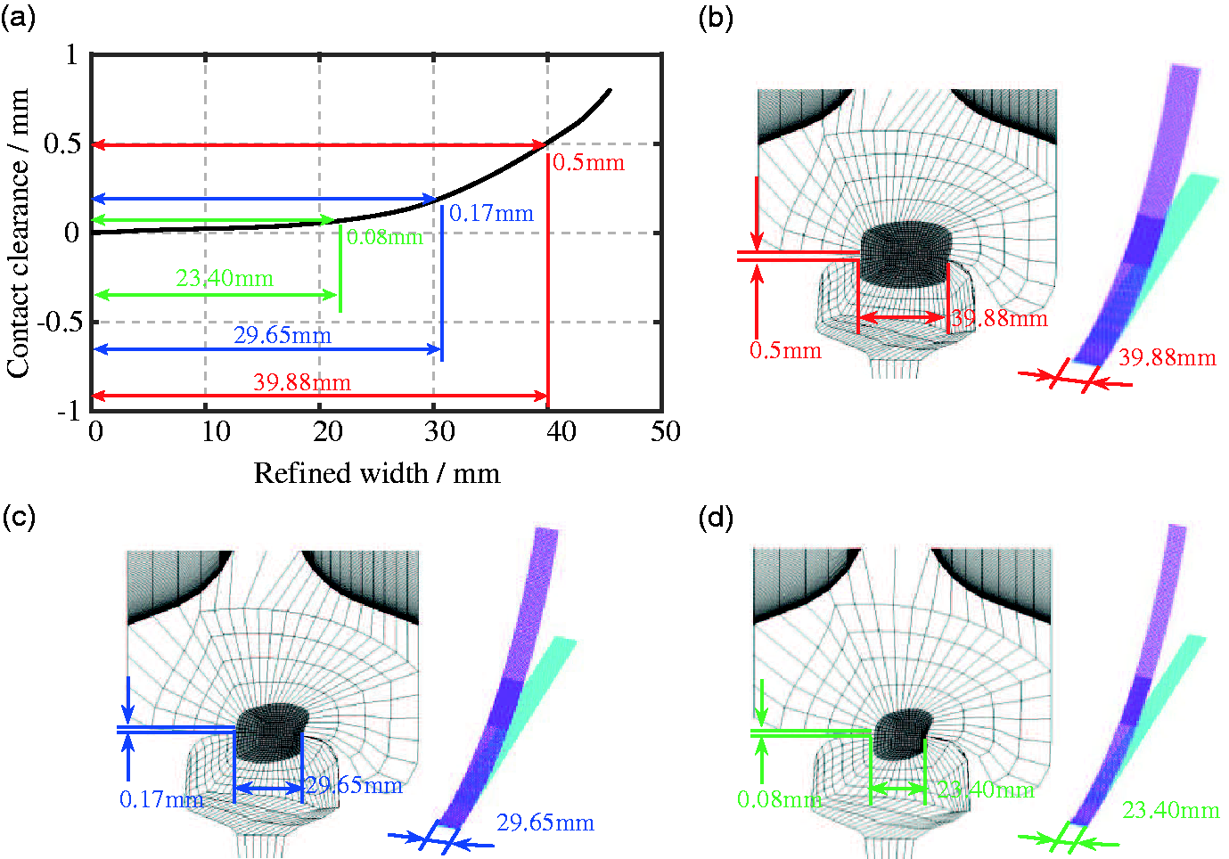

Since the actual contact areas would not vary much (i.e. the same axle load is applied in both implicit and explicit FE analyses), the effect of varying contact clearances δz on the performance of FE models would only be analysed by the implicit FE codes (i.e. no explicit analyses are performed).

Figure 12 shows the variation of normal pressure corresponding to different contact clearances. A noticeable discrepancy of the maximum contact pressure is observed between Cases I (1216 MPa) and II (1041 MPa). Such a discrepancy is explainable, since the mesh sizes of FE models at the origin of wheel rotation (not the solution area, see Figure 1) are relatively large (around 2 mm). Also, considering that W/R contact occurs at a highly stressed area (i.e. as small as 150 mm², see Ma et al.³⁵), these large mesh sizes are hardly possible to capture the stress/strain gradients accurately. It can thus readily trigger the tolerable discrepancies of the maximum contact pressure. (Notation: the contact responses extracted from the solution area, where the mesh size is as small as 1 mm, are preferred.)

Figure 12.

Variation of actual contact patches and contact pressure with respect to different refined widths: (a) Case I: δz = 0.5 mm, Δy = 39.88 mm. (b) Case II: δz = 0.17 mm, Δy = 29.65 mm and (c) Case III: δz = 0.08 mm, Δy = 23.40 mm.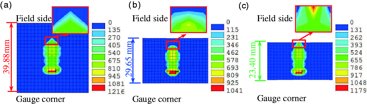

With respect to Case III ( $δ z = 0.08$ mm, Figure 12(c)), it can be observed that the refined potential contact area cannot fully cover the one simulated by the model any more. It indicates that the accuracy of contact solution might not be guaranteed, which is attributed to the underestimation of the size of refined potential contact area.

Moreover, it can be observed from Table 2 that the amount of the discretised elements as well as the calculation expense reduce significantly with the decrease of the contact clearance δz. Taking both the calculation expenses and the accuracy into account, the contact clearance of 0.17 mm appears to be a good choice for the operational conditions as described in the 2D-Geo analysis section.

To assess the applicability of the selected contact clearance (0.17 mm) to varying axle loads, two more case studies with axle load of 120 kN and 140 kN have been performed. Figure 13 shows the comparison of actual contact patches with respect to different axle loads. It can be seen that there is a steady increase in both the maximum contact pressure and the actual contact area in relation to the increasing axle loads. The width of refined potential contact areas determined by the contact clearance of 0.17 mm is robust enough to encompass all the real contact areas, which are resulting from the applied axle loads up to 40% (140 kN) higher than the normal one (100 kN).

Figure 13.

Comparison of actual contact patches and contact pressure at different axle loads: (a) 100 kN. (b) 120 kN and (c) 140 kN.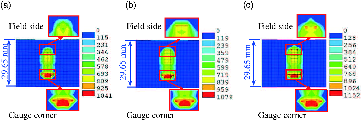

Similarly, the applicability of the selected contact clearance of 0.17 mm to the varying lateral shifts of the wheel-set (see Figure 9) has been evaluated. The results are shown in Figure 14(a) to (c). It can be seen that although the contact clearance of 0.17 mm can satisfy the case with the lateral shift of 5.5 mm (Figure 14(c)), it is insufficient for the case of −5.5 mm (Figure 14(a)), where the real contact patch tends to fall out of the refined potential contact area. Given a larger contact clearance δz of 0.35 mm, it is observed from Figure 14(d) that the refined potential contact area is able to better encompass the real contact area.

Figure 14.

Comparison of actual contact patches and contact pressure at different lateral shifts: (a) −5.5 mm (δz = 0.17 mm); (b) 0.0 mm (δz = 0.17 mm); (c) 5.5 mm (δz = 0.17 mm); and (d −5.5 mm (δz = 0.35 mm).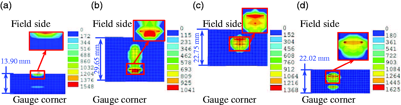

In summary, a contact clearance of 0.17 mm performs well at zero lateral displacement of the wheel-set. It is robust enough to apply in the cases of higher axle loads. One can further affirm that such a contact clearance is applicable to the case of different operational conditions (i.e. train velocities, friction coefficients, traction coefficients, etc.), since their influences on the size of real contact patches are insignificant in comparison to the increased axle loads. The applicability of contact clearance 0.17 mm to these varying operational patterns has been verified in the authors’ recent work.^32,35

However, with respect to the cases of large (e.g. δy = −5.5 mm, contact occurs between rail gauge corner and wheel flange root) lateral displacements of the wheel-set, this contact clearance of 0.17 mm is no longer suitable. A contact clearance of 0.35 mm is thus suggested based on the simulation results. It has better robustness than that of 0.17 mm, which implies that the contact clearance of 0.35 mm has wider applicability to different geometrical, loading, operational conditions of the W/R interaction.

In extreme cases (e.g. severe worn contact geometries), if the suggested contact clearance (either 0.17 mm or 0.35 mm) cannot guarantee good results, it is recommended to follow the above presented parametric study procedure to make a good decision. Normally within two (maximally three) times of targeted parametric examinations of contact clearances, the best refined width of the potential contact area can be found.

Travelling distance

Apart from the contact clearance δz, the dimensions of the potential contact area can be changed by adjusting another important parameter: travelling distance d. The dynamic behaviour of W/R interaction is studied from an initial travelling distance of 660 mm. Note that the interface parameters (such as contact stiffness and damping) are chosen as default.

Figure 15(a) shows the results of contact forces obtained from implicit-to-explicit FE analyses. It can be observed that the W/R mutual reactions are equal in magnitude and opposite in direction. Such observations are complementary to the classical contact theory as demonstrated in McMichael.³⁶

Figure 15.

(a) Responses of W/R contact forces with a travelling distance (d) of 660 mm; (b) schematic graph of the W/R interaction and (c) close-up view on the reactions at contact point CP.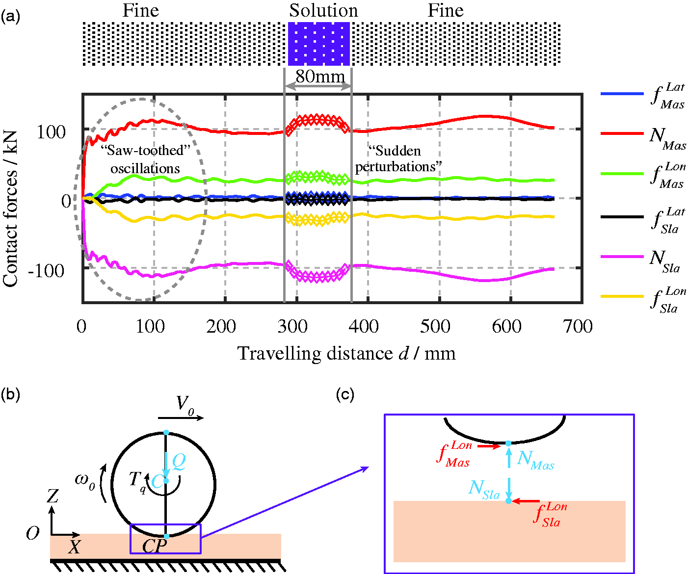

The solid lines represent the contact response in the dense meshed area, while the diamond dotted lines denote that inside the solution area. It is observed that the vertical contact forces N_Mas and N_Sla vary around the prescribed axle load (100 kN). Here, the subscripts “Mas” and “Sla” are the abbreviations of “Master” and “Slave”, which refer to the resulting contact forces on the master and slave contact interfaces, respectively. The “saw-toothed” oscillations of N_Mas and N_Sla (as denoted by the grey elliptical box) gradually decay at the first 150 mm from the starting point. These noticeable oscillations are mainly caused by the initial conditions (i.e. the applied initial train velocities, accelerations, etc.) according to the authors’ earlier research.³⁵ With the increase of initial velocities, the oscillation amplitudes will increase correspondingly.

In addition, the longitudinal frictional forces of $f_{Mas}^{Lon}$ and $f_{Sla}^{Lon}$ grow gradually to its saturation value 25 kN, which is in line with the applied traction. Due to the constrained lateral motion of the wheel-set and small contact angle between the resultant W/R contact geometries at the lateral shift of 0 mm, the lateral force components $f_{Mas}^{Lat}$ and $f_{Sla}^{Lat}$ seem to make minor contribution (varying around 0 kN). Here, the superscripts “Lon” and “Lat” are the abbreviations of “Longitudinal” and “Lateral”.

In comparison with the dense meshed region (see Figure 15(a)), all the force components exhibit a “sudden perturbation”, as the wheel rolls and approaches the vicinity of the solution area (80 mm). The causes of these “sudden perturbations” have been studied extensively and found (see supplement material)³⁵ to be the difference of the associated mesh sizes, which vary from 2 mm (the dense meshed area) to 1 mm (the solution area). For this reason, the magnitude of nodal contact stiffness 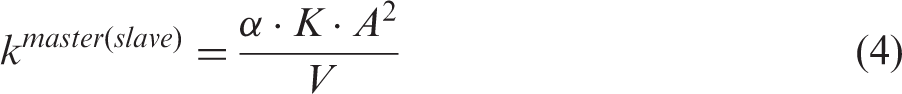$k^{master (slave)}$ , which is expressed as²¹

k^{master (slave)} = \frac{α \cdot K \cdot A^{2}}{V}

(4) is thus strongly affected. Here, α denotes the penalty scale factor, K is the bulk modulus, V and A represent the volume and face area of a contact element, respectively.

Accordingly, the change of contact stiffness manifests itself in the variation of contact forces f, which are then calculated on the basis of penalty method²¹

f = k^{master (slave)} l

(5)

Here, l is the amount of penetrations between master and slave segments.

To sum up, the variation of mesh sizes implies the “sudden perturbations” of contact forces as shown in Figure 15(a). Also, it has been reported in Ma et al.³⁵ that the problems of “sudden perturbations” can be addressed using an optimal penalty scale factor α (i.e. $α = 12.8$ ), which is determined according to the criteria of contact stability.^21,35

To investigate the sensitivity of contact solutions to the travelling distance d, five cases of travelling distance varying from 240 mm to 800 mm are selected and analysed. The information about the obtained FE models is listed in Table 3.

Table 3.

Comparison of FE models with respect to different travelling distances.

	Variables			FE models^a
Cases	δz (mm)	d (mm)	ɛ ₀	N ^b	T^c (h)
I	0.17 (best)	800	0	373,511	25.3
II		660		323,879	19.6
III		520		275,043	12.5
IV		380		225,033	7.7
V		240		176,205	4.7

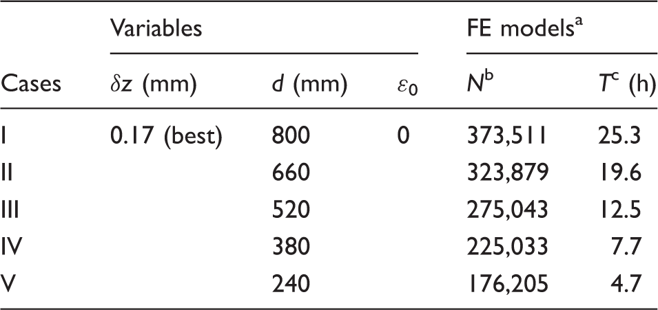
Implicit-to-explicit sequential solution.

Number of elements.

Calculation expense.

Figure 16(a) shows three of the five representative refined FE models with the travelling distance of 240, 520 and 800 mm, respectively. A close-up view on the performance of these varying travelling distances is taken by a supplemental and independent check on the resulting contact forces (as suggested by McMichael³⁶). The results shown in Figure 16(b) indicate that all the resulting vertical forces are varying around the axle load (100 kN) exerted on the wheel axle. It is clear that the oscillations of contact forces (“sudden perturbations” as depicted with diamond dotted lines) occur for all the five cases of different travelling distances.

Figure 16.

Influence of varying travelling distances on the W/R dynamic contact responses: (a) representative FE models of the different travelling distances and (b) vertical contact force with respect to different travelling distances.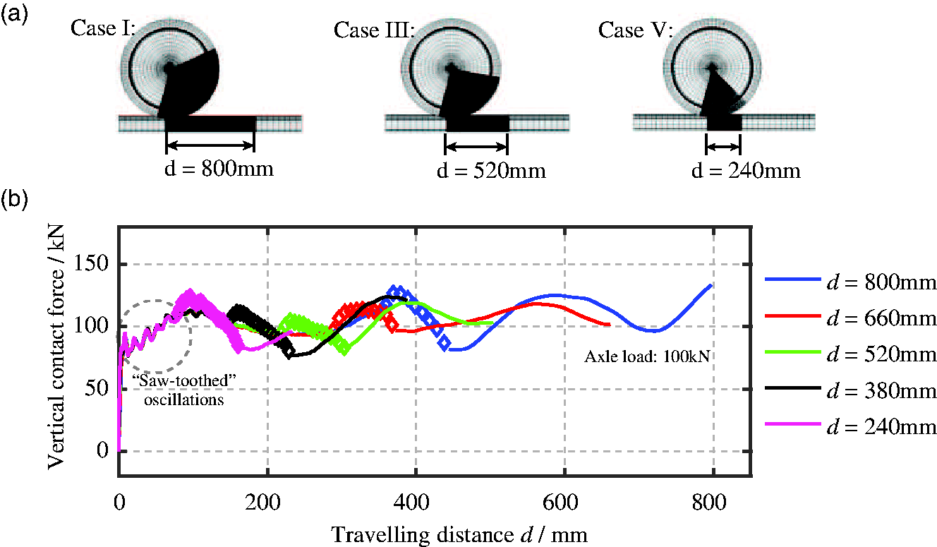

Similarly, the “saw-toothed” force oscillations, which have been explained previously, are observed in Figure 16(b). Also, it can be seen that all the FE models take around 150 mm to completely get rid of the initial contact disturbances under the specified operational conditions as shown in Table 1.

Figure 17 shows the normal contact pressure that is extracted at the instant when the wheel travels over the middle of the solution area. It can be seen that both the magnitude and the distribution of the contact pressure vary slightly with respect to different travelling distances.

Figure 17.

Effect of varying travelling distances on contact pressure.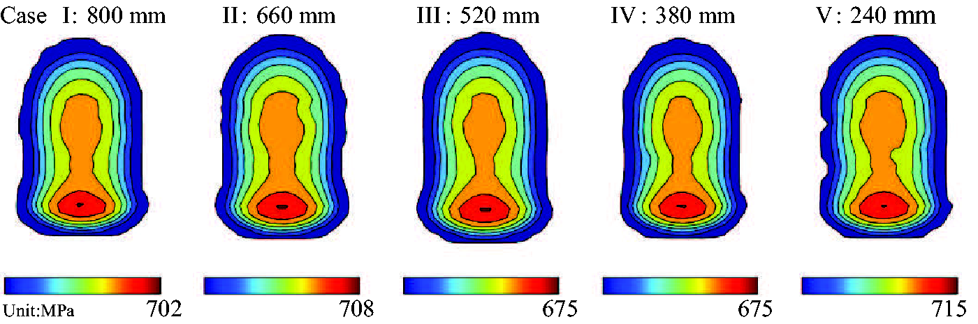

In view of the increasing calculation expense (as listed in Table 3) as well as the varying contact forces and pressures, it is practically necessary to build up a guideline/criterion to select the best travelling distance. Aiming to maintain the good compromise between the calculation efficiency and accuracy, the guideline is formulated as a recommendation:

The overall travelling distance should be kept shorter enough to save the calculation expenses.

A distance of 150 mm before the solution area should be reserved for damping out the “saw-toothed oscillations”.

Following the aforementioned guideline, the most suitable travelling distance of 520 mm is suggested. This suggested that the travelling distance d would be used for W/R contact analysis in the rest of this paper.

Initial slip

To study the influence of initial slips ɛ₀ on the dynamic performance of W/R interaction, a series of FE simulations have been performed. The contact clearance δz (0.35 mm) and travelling distance d (0.52 m) suggested are used, while the initial slips ɛ₀ vary from −0.04 to 0.13.

Figure 18 shows the variation of longitudinal frictional forces with respect to different initial slips ɛ₀. Figure 19 shows the effect of varying initial slips on the distribution of shear stresses. It is clear that both the frictional forces and the shear stresses change significantly with respect to the initial slips, which implies the unexpected initial slip ɛ₀ has a significant influence on the tangential solutions of W/R interaction.

Figure 18.

Variation of frictional forces with respect to different initial slips.

Figure 19.

Effect of varying the initial slips on the surface shear stress.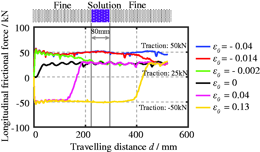

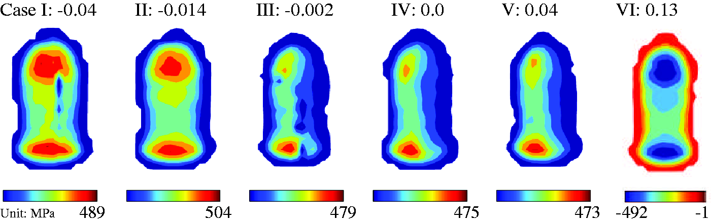
With the increase of initial slips ɛ₀ from −0.04 to −0.002 (i.e. the first three cases), the magnitude of longitudinal frictional forces tends to drop from 50 kN to 25 kN (see Figure 18). Accordingly, the distribution of shear stresses changes. For Cases I ( $ɛ_{0} = - 0.04$ ) and II ( $ɛ_{0} = - 0.014$ ), the shear stress is distributed parabolically all over the contact patch. Regarding Case III ( $ɛ_{0} = - 0.002$ ), the “hot area” of shear stress is significantly reduced. Here, “hot area” is referred to as an area, where the amplitude of the shear stress is larger than 250 MPa. Such a “hot area” is positioned at the rear part of the contact patch.

Similar patterns of shear stress distribution occur in the other two cases, Cases IV ( $ɛ_{0} = 0.0$ ) and V ( $ɛ_{0} = 0.04$ ). The reduced “hot area” of shear stress manifests itself in the small value (25 kN) of longitudinal frictional forces (see Cases III–V in Figure 18).

When the value of ɛ₀ becomes positive (i.e. Cases V ( $ɛ_{0} = 0.04$ ) and VI ( $ɛ_{0} = 0.13$ )), negative longitudinal forces (−50 kN) are observed. These negative frictional forces hold constant for a certain travelling distance or time span (i.e. the calculation time). After that, it steeply increases and then reaches a steady state, getting saturated with a positive frictional force of 25 kN. The distance/time, that the negative frictional forces hold, is highly related to the magnitude of initial slips. More specifically, the larger the value of $| ɛ_{0} |$ is, the longer distance/time the wheel has to travel so as to accomplish such conversions of frictional forces (see Figure 18).

Such phenomena could be explained by the wheel kinematics as shown in Figure 20, which depicts the relationship between the frictional forces and the slip velocities. It can be seen that the directions of frictional forces are in opposite to the ones of slip velocities. Thus, the magnitude of frictional forces changes from negative to positive in the Cases V and VI, where the initial slips are positive as opposed to the others.

Figure 20.

Schematic of the wheel kinematics: (a) negative initial slip 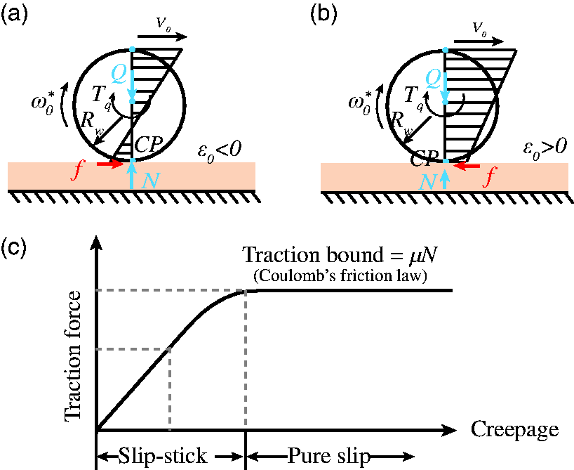$ɛ_{0} <$ 0; (b) positive initial slip $ɛ_{0} >$ 0 and (c) traction curve adapted from Esveld.²⁵

Figure 20(c) schematically shows the traction curve.²⁵ It is observed that when the magnitude of the slip (also interpreted as creep-age) exceeds certain level, the regime of full slip is entered. The frictional force thus reaches its saturation value (i.e. traction bound of 50 kN). Here, the traction bound, which amounts to the product of frictional coefficient μ and the normal load N, is determined by Coulomb’s friction law. This indicates the trend in the results of frictional forces shown in Figure 18, where all the six cases tend to converge over travelling distance/time towards a steady state of partial slip. It also implies that for the cases of non-zero initial slips, the contact statuses first fall into full slip and then approach the equilibrium state of partial slip. This state, in which the expected frictional forces is equal to the applied one of 25 kN (see equation (3)), can only be reached until the effect of the unexpected initial slip has been completely damped out.

For the case of initial slip ɛ₀ = 0 (i.e. Case IV: initial velocities applied appropriately), the accurate tangential contact solution can be obtained within a rather short travelling distance of 50 mm. If the absolute value of initial slip is small (e.g. Cases III and V), extra calculation time and travelling distances will be taken to ensure the correct solution. However, in the cases of large initial slips (e.g. Cases I, II, VI), the results of shear stress extracted from the solution area (80 mm) are inaccurate, which may lead to wrong decisions.

To summarise, using the proposed ‘eFE-CS’ approach, the local wheel rolling radius R_w can be correctly estimated. No unexpected initial slips will be introduced into the FE model. Accordingly, accurate and steady tangential solutions of W/R rolling contact problems can be guaranteed. It is thus recommended to address the issues of initial slip with the aid of this ‘eFE-CS’ strategy.

Discussion: Pros and cons of ‘eFE-CS’ model

From the results of the FE simulations presented, it can be noticed that the proposed ‘eFE-CS’ strategy is promising enough for improving the performance of FE simulations on W/R interaction. The advantages it holds can be categorised into four groups:

All the modelling challenges (see Challenges of FE analysis section), from which most of 3D-FE models often suffer, can be readily addressed. Also, a good compromise between the calculation accuracy and efficiency is maintained.

More detailed normal and tangential contact solutions than those of 2D W/R contact analysis^37,38 are generated. These stress/strain responses are expected to contribute positively on other advanced applications (e.g. prediction of wear/rolling contact fatigue, profile design/optimisation, etc.).

The dynamic effects, which are often neglected in the static or quasi-static 3D FE models¹³ (contact constrains are enforced with Lagrange Multiplier method, Arbitrary Lagrangian Eulerian method, etc.), are taken into account in the present model (Penalty method). A high degree of realism is attained.

The strategy shows good applicability to the problem of W/R interaction. As there are no special restrictions imposed upon its use, it is recommended to use for addressing other contact/impact problems (e.g. gear, bearing, metal forming, etc.) that have complex contact geometries.

Although the developed ‘eFE-CS’ model has many advantages, there is room remained to further increase its degree of realism and accuracy. For instance,

To enhance the steering capability: In the present ‘eFE-CS’ model, the steering capability of the wheel is limited, since the yaw motion is not allowed and only roll motion is considered. For this reason, it would be difficult to study the cases of W/R interaction at sharp curves (curve radius of 500 m or even small). In the future work, it is motivated to integrate several torsional control units onto the wheel for the purpose of attaining a sufficient steering capability.

To account for the accumulation of wheel passages: It is known that the degradation of W/R interface is due to cyclic contact loadings. To better predict the degradation process, the modelling of multiple wheel passages³⁹ is increasingly demanded.

To study the effect of second wheel of the axle: Using a half W/R FE model, the second wheel of the axle will have a mirrored roll angle and contact conditions, which correspond less well to the reality. As a consequence, the accuracy of the FE simulations would be adversely affected. For a more quantitative explanation in terms of how the mirrored contact conditions affect the contact solutions, rigorous verifications on the half W/R FE model against the complete wheel-set/track FE model are needed to be performed in the future work.

Conclusions

Aiming to improve the performance of FE analysis on the wheel–rail interaction, a new ‘eFE-CS’ strategy, that couples the 3D-FE model and the 2D-Geo contact model, has been presented. Prior to the 3D-FE simulations, the 2D-Geo contact analysis is performed to better define the contact properties that are in demand for FE analyses. Both the advantages and disadvantages of the developed ‘eFE-CS’ model have been discussed. Based on the simulation results and discussions, the following conclusions are drawn:

Following the coupling procedure, the convergence problems or even a failure of the FE simulations in the presence of gaps or penetrations have been addressed by correctly placing the wheel onto a position of “Just-in-contact” over the rail.

In order to avoid the issues of the redundant, insufficient or mismatched mesh refinement in the vicinity of the contact region, which will lead to either the prohibitive calculation expense or the inaccurate solution, an adaptive mesh refining technique based on the contact clearance has been proposed. Using this technique, the solution of W/R rolling frictional contact is able to be maintained with good accuracy and efficiency. The flexibility of this coupling approach has also been demonstrated by solving the cases of different contact locations due to various lateral shifts of the wheel-set.

An unexpected initial slip can be introduced by mismatching the angular and translational velocity of the wheel, owing to the wrongly estimated local wheel rolling radius. Such an initial slip can cost unnecessary calculation effort to achieve the steady frictional rolling state or even lead to wrong tangential solution of W/R interaction in extreme cases. Using the coupling strategy, the value of undesired initial slip can be easily minimised. Accordingly, the accurate and efficient FE solution can be guaranteed.

In conclusion, the proposed coupling strategy allows the proper prescription of the contact properties, which can enhance the performance of the FE analyses of W/R interaction significantly. Such a strategy is promising enough to promote the application of the FE approaches on the contact problems with more complex and irregular contact geometries (e.g. the mild or severe worn W/R interfaces, metal forming, gear, bearings, etc.).

Footnotes

Acknowledgements

The comments and suggestions from Prof. Rolf Dollevoet on the manuscript are gratefully acknowledged. Special thanks go to Dr Hongxia Zhou for critically reading this manuscript and giving helpful suggestions. The authors are also very grateful to all the reviewers for their thorough reading of the manuscript and for their constructive comments, which have helped to improve the manuscript.

Declaration of Conflicting Interests

The author(s) declared no potential conflicts of interest with respect to the research, authorship, and/or publication of this article.

Funding

The author(s) disclosed receipt of the following financial support for the research, authorship, and/or publication of this article: Yuewei Ma thanks the CSC (China Scholarship Council) for their financial support.

Supplementary Material

Supplementary material is available for this article online.

References

Huang

et al.

Methods to calculate accurate wheel/rail contact positions and static contact stress levels. Proc IMechE, Part F: J Rail and Rapid Transit 2016; 230: 138–150.

El-Ghandour

Hamper

Foster

. Coupled finite element and multibody system dynamics modeling of a three-dimensional railroad system. Proc IMechE, Part F: J Rail and Rapid Transit 2016; 230: 283–294.

Vollebregt EAH. User guide for contact, Vollebregt & Kalkers rolling and sliding contact model. VORtech, Techical Report TR09-03, version, 2013. Available at: https://www.kalkersoftware.org.

Carter

. On the action of a locomotive driving wheel. Proc R Soc London A 1926; 112: 151–157.

Harewood

McHugh

. Comparison of the implicit and explicit finite element methods using crystal plasticity. Comput Mater Sci 2007; 39: 481–494.

Sun

Lee

. Comparison of implicit and explicit finite element methods for dynamic problems. J Mater Process Technol 2000; 105: 110–118.

Wiest

Kassa

Daves

et al.

Assessment of methods for calculating contact pressure in wheel–rail/switch contact. Wear 2008; 265: 1439–1445.

Pun

Kan

Mutton

et al.

Ratcheting behaviour of high strength rail steels under bi-axial compression–torsion loadings: experiment and simulation. Int J Fatigue 2014; 66: 138–154.

Mandal

Dhanasekar

. Sub-modelling for the ratchetting failure of insulated rail joints. Int J Mech Sci 2013; 75: 110–122.

10.

Bijak-Żochowski

Marek

. Residual stress in some elasto-plastic problems of rolling contact with friction. Int J Mech Sci 1997; 39: 15–32.

11.

Telliskivi

Olofsson

Sellgren

et al.

A tool and a method for fe analysis of wheel and rail interaction, Stockholm, Sweden: Royal Institute of Technology (KTH), 2000.

12.

Ringsberg

Loo-Morrey

Josefson

et al.

Prediction of fatigue crack initiation for rolling contact fatigue. Int J Fatigue 2000; 22: 205–215.

13.

Ren

et al.

Optimal analysis on rail pre-grinding profile in high-speed railway. Jixie Gongcheng Xuebao (Chin J Mech Eng) 2012; 48: 90–97.

14.

Hughes

TJR

Taylor

Sackman

et al.

A finite element method for a class of contact-impact problems. Comput Methods Appl Mech Eng 1976; 8: 249–276.

15.

ANSYS, Inc. Ansys user’s manual: structural analysis guide, USA: ANSYS, Inc., 2013.

16.

. Introduction to the explicit finite element method for nonlinear transient dynamics, Hoboken, New Jersey, USA: John Wiley & Sons, Inc, 2012.

17.

Zhao

. The solution of frictional wheel–rail rolling contact with a 3D transient finite element model: validation and error analysis. Wear 2011; 271: 444–452.

18.

Tieu

Zhu

et al.

A 3d dynamic model to investigate wheel–rail contact under high and low adhesion. Int J Mech Sci 2014; 85: 63–75.

19.

Pletz

Daves

Ossberger

. A wheel set/crossing model regarding impact, sliding and deformation – explicit finite element approach. Wear 2012; 294: 446–456.

20.

Wen

Jin

Zhang

. Contact-impact stress analysis of rail joint region using the dynamic finite element method. Wear 2005; 258: 1301–1309.

21.

Hallquist JO. ANSYS/LS-DYNA theoretical manual. Livermore Software Technology Corporation, Livermore, California, USA, 2005.

22.

Kalker

. Three-dimensional elastic bodies in rolling contact 1990; vol. 2Germany: Springer Science & Business Media.

23.

European Committee for Standardization (CEN). EN 13715: 2006 + A1: 2010: railway applications – wheelsets and bogies – wheels – tread profile. UK: European Standard, 2006.

24.

International Union of Railways (UIC). UIC Leaflet 515-1 OR: passenger rolling stock – trailer bogies – running gear – general provisions applicable to the components of trailers bogies, 2nd ed. France: International Union of Railways, 2003.

25.

Esveld

. Modern railway track 2001; vol. 385The Netherlands: MRT-Productions Zaltbommel.

26.

Walker

. Fundamentals of physics extended, Hoboken, New Jersey, USA: John Wiley & Sons, Inc, 2010.

27.

Ma Y, Mashal AA and Markine VL. Numerical analysis of wheel-crossing interaction using a coupling strategy. In: Proceedings of the 3rd international conference on railway technology: research, development and maintenance (ed J Pombo), Cagliari, Italy, 5–8 April, pp.1–19. Stirlingshire, UK: Civil-Comp Press.

28.

Mashal

Markine

. Modelling and experimental validation of dynamic impact in 1:9 railway crossing panel. Tribol Int 2018; 118: 208–226.

29.

Ma Y and Markine VL. A numerical procedure for analysis of w/r contact using explicit finite element methods. In: CM2015: 10th international conference on contact mechanics, Colorado Springs, USA, 30 August–3 September 2015, pp.1–10.

30.

Shevtsov IY. Wheel/rail interface optimisation. PhD Thesis, Delft University of Technology, 2008.

31.

Zhang

Kong

. Effect of lateral displacement on elasto-plastic stress field in rail head. J Railway Eng Soc 1999; 16: 17–20.

32.

Markine

Mashal

et al.

Modelling verification and influence of operational patterns on tribological behaviour of wheel–rail interaction. Tribol Int 2017; 114: 264–281.

33.

Matsumoto

Sato

Tantmoto

et al.

Experimental and theoretical study on the dynamic performance of steering bogie in sharp curve. Veh Syst Dyn 1998; 29: 559–575.

34.

Benson

Hallquist

. A single surface contact algorithm for the post-buckling analysis of shell structures. Comput Meth Appl Mech Eng 1990; 78: 141–163.

35.

Markine

Mashal

et al.

Effect of wheel–rail interface parameters on contact stability in explicit finite element analysis. Proc IMechE, Part F: J Rail and Rapid Transit 2017.

36.

McMichael LD. Contact interface verification for dyna3d scenario 1: basic contact. Technical Report, Lawrence Livermore National Laboratory (LLNL), Livermore, CA, 2006.

37.

Markine

Steenbergen

MJMM

Shevtsov

. Combatting RCF on switch points by tuning elastic track properties. Wear 2011; 271: 158–167.

38.

Wan

Markine

Shevtsov

. Analysis of train/turnout vertical interaction using a fast numerical model and validation of that model. Proc IMechE, Part F: J Rail and Rapid Transit 2014; 228: 730–743.

39.

Thompson

. An investigation into rail corrugation due to micro-slip under multiple wheel/rail interactions. Wear 2005; 258: 1115–1125.

Improving the performance of finite element simulations on the wheel–rail interaction by using a coupling strategy

Abstract

Keywords

Introduction

W/R 3D-FE model

Discretised FE model

Challenges of FE analysis

Geometrical gaps/penetrations

Preload application

Mesh refinement

Coupling strategy

2D-Geo analysis

Coupled interface

“Zero” gaps/penetrations and obtained Rw

New adaptive mesh refinement

Flexibility of the new mesh refining approach

Resulting contact pairs

FE results and discussion

Contact clearance

Travelling distance

Initial slip

Discussion: Pros and cons of ‘eFE-CS’ model

Conclusions

Footnotes

Acknowledgements

Declaration of Conflicting Interests

Funding

Supplementary Material

References

“Zero” gaps/penetrations and obtained R_w