Goal oriented trajectory prediction conditioned on reachable road context

Abstract

Trajectory prediction of surrounding traffic agents is crucial for autonomous vehicles to perform collision-free and efficient planning at urban intersections. Despite interactions with neighbour objects, road layout information plays an essential role in improving prediction accuracy and enhancing the interpretability of prediction models. However, exploring reachable areas and effectively leveraging these contextual clues in predictions remain challenging. In this work, a goal-oriented trajectory prediction framework is proposed to integrate valuable road layout information. The framework leverages sparse and non-uniform map elements to represent moving intentions. For effective exploration of relevant map elements, a constrained breadth-first search is proposed, enabling simultaneous and efficient exploration across lateral and longitudinal directions by incorporating behavioural constraints. The attention mechanism and a dynamic mask are combined to focus on the most relevant map element features and predict corresponding goal points, facilitating the final trajectory prediction. This progressive narrowing of the inference space enhances both the accuracy and interpretability of the prediction model. Experimental results on the Intersection Drone Dataset and Roundabout Drone Dataset demonstrate that the proposed model achieves a 73.1% accuracy in predicting the most likely map elements, with an average displacement error below 0.75 m and a final displacement error around 1.95 m with a prediction horizon of 4 s.

Introduction

Accurate long-term trajectory prediction of surrounding traffic agents is crucial for autonomous vehicles to navigate complex driving scenarios safely, particularly at urban intersections where traffic dynamics are highly interactive and uncertain. ¹ Extensive research has focused on modelling interactions between target agents (TAs) and surrounding agents (SAs) using deep learning (DL) techniques, such as Convolutional Neural Networks (CNNs), ² Graph Neural Networks (GNNs) ³ and the Attention Mechanism (AM),^4–6 which effectively capture spatial-temporal dependencies. Concurrently, it is equally important to integrate geometric and semantic information of road layouts (RL), which can guide predictions by following lane geometry, connectivity, and other constraints influencing the TA’s manoeuvres.^7,8 However, urban intersections present unique challenges that have not been adequately addressed by existing approaches, hindering the integration of RL information into prediction backbones.

Urban intersections are usually characterised by sparse vectorised map representations, where map elements spatially overlap despite being topologically distant. This spatial-topological discrepancy poses distinct difficulties in efficient and lightweight reachable area exploration and destination-oriented context extraction.

Related work

The influence of RL maps can be evaluated by adding map-aware features as additional inputs, for example, the TA’s deviation from the lane centreline or lane markings. ⁹ Though easy to implement, this implicit feature mining approach can lead to a large and heterogeneous input vector, making it difficult for monolithic NNs to efficiently extract and abstract road-related features.

One alternative is to discretise the road scene around the TA into rasterisation images or multiple-channel grid maps in Bird-Eye-View (BEV) and apply CNNs for spatial feature extraction.^10–13 These image-like representations are intuitive and preserve local traffic scene contexts. ¹⁴ Nevertheless, they struggle with representing long-range topologies, are often storage-intensive and can be less efficient in real-time applications.^3,15,16 Besides, it is hard to realise a topology-guided feature exploration.

A more structured approach is to organise the RL map as a graph, where each node corresponds to a lane segment and edges are built based on agents’ traversability across lane segments. A lane segment is usually represented by a sequence of ordered polyline points, either from centrelines or boundaries.^15,17 This vectorised representation is sparser than image-based methods while retaining the RL topology and the map graph allows message passing along the RL topology using GNNs. ¹⁸ For example, Liang et al. ³ aggregate vehicle and lane node embeddings and apply a Graph Convolutional Network (GCN) to propagate this contextual information over the map graph. Similar techniques have been effectively applied in literature, enabling global topology information to be captured.^7,19,20

However, to reach a topologically far node, there is a risk of over-smoothing while performing multi-step message propagation along the map graph, where node features tend to become indistinguishable after multiple aggregation steps and the quality of feature representation degrades. ³ Another issue is that relating the TA to the most relevant lane nodes can be non-trivial when multiple spatially overlapping lane segments are present, potentially leading to incorrect agent-lane assignments. A wrong match might cause incorrect feature concatenation because overlapped lane nodes are close in the Euclidean space, but far from each other in the RL topology. Moreover, many existing works combine RL features with those of the TA in a black-box manner and introduce data from irrelevant RL elements, providing limited interpretability regarding how RL information informs the TA’s predicted manoeuvres.

To address these limitations, some studies have proposed two-stage approaches. ⁸ The first stage aims to identify the lanes and lane points that are relevant to the prediction, that is, that are likely to be reached within the prediction horizon, starting from the given position of the TA. These generated intermediate outputs can be interpreted as the intention of TA and are then used to guide the final prediction in the following stage.

Lane instances within a customised distance centred at the TA are usually relevant, where lane candidates are selected by a range search (RngS). With these prior selected lanes, Pan et al. ²¹ calculate their importance through MLP based on the historical and current deviations from the TA to the lane centrelines. In contrast, Luo et al. ²² and Liu et al. ²³ calculate their probability of reachable lanes by dot-product based on the TA’s historical encoding and lane encodings. With candidate lanes and their scores, AMs are usually used to fuse the encodings of the TA and of the candidate lanes, which further contributes to trajectory prediction. A significant advantage of AM over GCN is that the features of individual lanes are preserved fully, without smoothing due to message propagation. However, most existing methods derive comprehensive lane element encodings solely through a weighted sum of relevant encodings without providing explanations for the assigned weights. This can lead to the selection of features from irrelevant lane instances, as evidenced by the work of Wang et al. ²⁴ While the model may still operate effectively under these conditions, it does not ensure learning from ideal data, like the ground truth, thereby potentially compromising interpretability.

To further narrow down the attention scope, lane pieces instead of complete lanes are selected for lane encoding abstraction. To get a concise map of interest, Gómez et al. ²⁵ select relevant lanes based on the RL topology and then prune them according to the TA’s current position and an estimation of its future travel distances. Taking advantage of a graph representation of the RL, Gao et al. ²⁶ perform depth-first-search (DFS) to identify relevant lane nodes starting from the currently occupied node. In the DFS, the maximum depth is limited according to the average speed of the TA. Kim et al. ¹⁷ apply an RngS with a range of 10 m to identify potential candidate lane segments and then use DFS to extend these lane segments by searching their predecessors and successors until a predefined distance is reached. In this combination, DFS is used to extend exploration in the longitudinal direction of the lanes while RngS is used to compensate for searching in the traversal direction. Though plausible lanes are identified, redundant information is included in the reverse moving direction and the lane representation is too rigid to describe manoeuvres like lane changing.

An alternative for selecting lanes or lane pieces is to estimate the goal point of the TA within the prediction horizon. For this purpose, Gu et al. ²⁷ select sample points on the best candidate lane and then use AM to select the candidate goal point. Lu et al. ¹⁹ pre-sample anchor points in the drivable area evenly and predict their probability directly, of which the top K points are selected to do final predictions. Gilles et al. ²⁸ select the most likely lane segments before estimating goal points within the chosen lane segments.

By estimating goal points according to RL maps, moving intentions have been embodied and interpretability has been improved. However, these methods rely either on pre-sampled anchor points as candidates^19,27 or the discretisation of selected lane pieces to estimate goal points. ²⁸ These operations are storage-intensive and limit the expression ability of NNs because of restricting the outputs of NNs to a discretisation space.

Motivations and contributions

Existing goal-oriented trajectory prediction methods rely heavily on continuous lane structures to illustrate primary motion intentions,^17,22,23 such as complete lane instances, consecutive lane segments, or immediate successors. These elements originate near the current position of the TA and extend to distant locations. However, these approaches lack flexibility in identifying destinations involving lane-changing manoeuvres, as continuous lane elements inherently restrict exploration to fixed pathways.

To overcome this limitation, sparse, fragmented lane segments—sometimes even distant ones—are used to represent coarse destinations, thereby avoiding reliance on predefined continuous lane structures.

When exploring the Area of Interest (AOI), existing search strategies often struggle to balance longitudinal lane-following and lateral lane-changing exploration. For example, commonly used methods like RngS indiscriminately include lane segments within a predefined circular radius.^22,29 This approach introduces lateral redundancy, as it depends on homogeneous Euclidean distance metrics, whereas effective longitudinal exploration typically requires larger radii. Conversely, DFS leverages the map’s graph structure to facilitate efficient longitudinal exploration within a specified distance threshold. ²⁶ However, supplementary lateral exploration mechanisms are still necessary in lane-changing scenarios. Methods such as RngS or K-Nearest Neighbours (KNN) are often combined with DFS to identify neighbouring lanes,^17,25 followed by longitudinal extension of the AOI along these selected lateral segments. Unfortunately, this hybrid search framework imposes additional computational and storage burdens.

To address these identified limitations, this research focuses on map data mining for accurate, efficient and interpretable trajectory prediction at urban intersections. A systematic framework is developed, grounded in domain-specific constraints. A unified Constrained Breadth-First Search (cBFS) approach is proposed to balance longitudinal search efficiency and lateral search relevance through a simultaneous process. To prevent excessive lateral exploration, a lateral search depth constraint is proposed based on realistic vehicle manoeuvring capabilities and statistical analysis of lane-change manoeuvres, which transforms BFS into a domain-adapted tool.

Building upon this refined AOI exploration, a goal-oriented trajectory prediction framework is introduced. This framework infers the moving intentions of TAs by scoring lane segments that the TA will reach in the AOI and subsequently estimating potential goal points, progressively narrowing down the search space.

Rather than propagating information across all reachable elements within AOI, AM is employed to establish a direct supervisory link between the traffic context and TA coarse intentions. This is achieved by estimating the most relevant map element and undergoing explicit training on ground-truth destination elements. However, cBFS may fail to identify an adequate number of map elements in specific edge cases, such as at map boundaries or when TAs operate off-road. To address these cases, a dynamic map mask is introduced that assigns a zero score to vacant positions in the AOI. This effectively excludes the influence of irrelevant map elements, enhances adaptability to both on-road and off-road agents, and stabilises the training process.

Subsequently, a goal estimation is performed based on context mining results from the map elements within the AOI. Unlike existing works that either pre-sample goal candidates across drivable areas or rely on the fusion of scenario features without explicit grounding in map elements,^30,31 the potential goal point is generated by focusing on the most influential map elements. This approach reduces the impact of less relevant map elements, an aspect often neglected in related studies.

The novel contributions of this paper are as follows:

• (1) A novel goal-oriented trajectory prediction framework is proposed. This framework leverages fragmented map elements to represent coarse moving destinations and employs a flexible map element mask to exclude the influence of less relevant elements and enhance the adaptability to TAs not following RLs, thereby ensuring stable performance.

• (2) A unified AOI exploration method, denoted as cBFS, is proposed based on BFS. cBFS incorporates behavioural lane-change constraints to facilitate effective and efficient simultaneous longitudinal and lateral exploration with lightweight storage. This mechanism eliminates the need for separate lateral/longitudinal search algorithms and ensures balanced and efficient exploration aligned with real-world driving constraints.

This work is significant to the intelligent transportation and autonomous driving communities because:

• (1) It provides an approach to efficiently mine road scene and interaction information, enhancing the prediction accuracy.

• (2) The interpretability of the prediction is improved by systematically refining the inference space from coarse map elements to goal points. The probabilities associated with the top map elements and their corresponding goal points provide insight into the model's understanding of moving intentions and subsequent destinations.

• (3) The proposed RL map exploration method can be adjusted with customised accumulated distance and lane-changing limitations, and thus can be generalised in various scenarios.

In the rest of this paper, Section ‘Methodology’ presents the methodologies to get data ready for model inputs. In Section ‘Prediction model,’ the goal-oriented trajectory prediction model is proposed. Experiments and results are reported and discussed in Section ‘Experiment evaluation’, followed by the conclusions drawn in Section ‘Conclusions’.

Methodology

The problem of trajectory prediction in this paper is formulated as determining the future trajectories of a TA conditioned on its positional data and corresponding useful scenario information (including neighbours and RL maps) at each discrete time step $t$ over a fixed-size historical horizon. Given observations $\mathit{X}$ in the form of past statuses and scenario info of the TA, the prediction model seeks to provide its future trajectory. In this research, the TA includes cars, buses and bicycles in urban scenarios, consisting of cross intersections and a roundabout.

Inputs and outputs

Formally, a set of observable features $\mathit{X}$ and a set of target outputs $\hat{\mathit{Y}}$ to be predicted are considered. It is assumed that all features can be accessed simultaneously at each time step and that historical measurements with a sequence length of $h+1$ are available, where $h$ is a fixed time horizon. Let ${\mathcal{T}}_{\mathrm{hist}}=\{0,\dots ,h\}$ and, for $k\in {\mathcal{T}}_{\mathrm{hist}}$ , the value of the TA’s status $k$ time steps earlier is denoted by ${\mathit{X}}^{(t-k)}$ . Similarly, define ${\mathcal{T}}_{\mathrm{pred}}=\{0,\dots ,f\}$ and, for $k\in {\mathcal{T}}_{\mathrm{pred}}$ , denote the value of output time steps in the future by ${\hat{\mathit{Y}}}^{(t+k)}$ . It is proposed to use a DL-based model, in which a regression function $F$ is trained such that the predicted outputs $\hat{\mathit{Y}}=F\left(\mathit{X}\right)$ match the actual values $\mathit{Y}$ as closely as possible.

The inputs to the model are a set of track histories and surrounding traffic information of the TA:

$$\mathit{X}=\left[\begin{array}{cccc}{\mathit{X}}^{(t-h)},\hfill & \dots ,\hfill & {\mathit{X}}^{(t-1)},\hfill & {\mathit{X}}^{\left(t\right)}\hfill \end{array}\right],$$

(1)

And at a time instant $t$ , for the TA, the following features are defined in ${\mathit{X}}^{\left(t\right)}$ :

• TA’s information $\mathit{TA}$ , including absolute position in the $x$ and $y$ direction with a local Cartesian coordinate and velocities in the $x$ and $y$ directions, denoted by $p_x$ , $p_y$ , $v_x$ and $v_y$ respectively,

• SAs’ information $\mathit{SA}$ , defined in equation (5) of Section ‘Neighbour information’,

• Map information $M_{\mathrm{cnl}}$ , defined in equation (6) of Section ‘Map information’,

  $${\mathit{X}}^{\left(t\right)}=[\mathit{T}{\mathit{A}}^{\left(t\right)},\mathit{S}{\mathit{A}}^{\left(t\right)},{\mathit{M}}_{\mathrm{cnl}}^{(t)}].$$

  (2)

Though velocity information has been implicitly included in the position values as a constant time interval is applied, the velocity values are used as additional inputs to the model input.

The output of the model is the predicted positions over the prediction horizon:

$$\hat{\mathit{Y}}=\left[\begin{array}{ccc}{\hat{\mathit{Y}}}^{(t+1)},\hfill & \dots ,\hfill & {\hat{\mathit{Y}}}^{(t+f)}\hfill \end{array}\right],$$

(3)

and at each time frame $t$ ,

$${\hat{\mathit{Y}}}^{\left(t\right)}=[{p_x}^{\left(t\right)},{p_y}^{\left(t\right)}]$$

(4)

represents the $x$ and $y$ coordinates at the time $t$ of the TA being predicted.

Neighbour information

It is common to arrange SAs in a grid which is centred at the TA and aligned to the TA’s moving direction. However, this rectangular grid shape does not conform to the actual road layout and is more expensive in storage in case it needs to be extended to cover SAs that do not move in the same direction as the TA, like in intersections. Considering this limitation, SAs in this research are identified by a range search and any surrounding agent within a range of 60 m is considered an SA.

This includes both static and kinetic objects and makes it more adaptable to complex traffic environments.

SAs’ information at the time $t$ is stored as below:

$$\mathit{S}{\mathit{A}}^{(t)}=\left[\begin{array}{c}{p_x}_1^{(t)},{p_y}_1^{(t)},{v_x}_1^{(t)},{v_y}_1^{(t)},\dots \hfill \\ \multicolumn{1}{c}{{p_x}_k^{(t)},{p_y}_k^{(t)},{v_x}_k^{(t)},{v_y}_k^{(t)},\dots }\\ \multicolumn{1}{c}{{p_x}_n^{(t)},{p_y}_n^{(t)},{v_x}_n^{(t)},{v_y}_n^{(t)}}\end{array}\right],$$

(5)

where $k\in [1,n]$ and $n$ denotes the maximum number of SAs. This is a fixed-size vector and the features of individual SAs are grouped together. The maximum number of SAs is set to be 15. ²⁹ If an SA is absent in the vector, zeros are filled instead.

Map information

This work focuses on urban intersections. Road layout and geometric information are provided in the Lanelet2 format. ³² In this representation, an atomic map element, like a piece of lane segment, is called a lanelet and is defined by sequential points of its two boundaries. These boundary points can be low-density, which contributes to a sparse and storage-efficient description. Totally, three interactions from the inD dataset (Intersections Drone Dataset) ³³ and one roundabout from the rounD dataset (Roundabouts Drone Dataset) ³⁴ are included.

Map data representation

For a more compact representation and easier extraction of map element features, the centrelines of lanelets are used instead of their boundaries in the description of road topologies and geometries. The centrelines are calculated by searching for maximal disks along the lanelets, which produces robust and smooth outputs.^35,36 An illustration of Lanelet2 maps of the target scenarios used in this research is shown in Figure 1.

Figure 1.

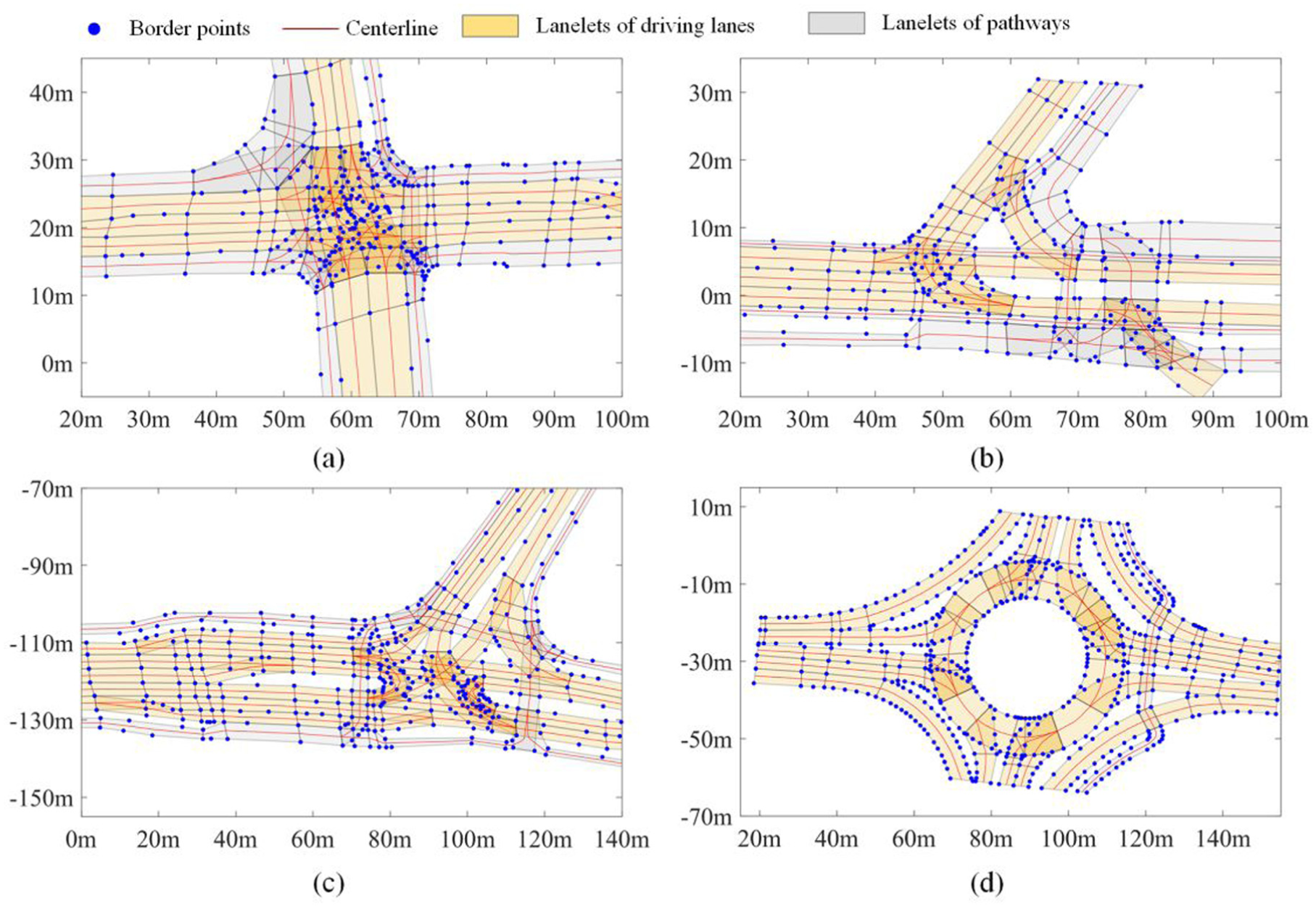
The target intersections are formatted in Lanelet2. Boundary points of lanelets are marked in blue and their centrelines are depicted in red. Lanes are represented by connected lanelets. Driving lanes and pathways are shown in light yellow and grey, respectively.

The centreline of a lanelet consists of several ordered centre points. To facilitate the application of CNN-based map feature extraction in Section ‘Map element feature encoder’, each centreline is down-sampled from a dense point representation and is composed of 18 centre points, the sequence of which is aligned with the driving direction.

With these definitions, the map $M_{\mathrm{cnl}}$ is an assembly of all lanelet centrelines in the target scenario, each consisting of multiple centre points represented by their coordinates:

$${\mathit{M}}_{\mathrm{cnl}}=[\mathrm{cn}{l}_1,\mathrm{cn}{l}_2,\dots ,\mathrm{cn}{l}_i,\dots ,\mathrm{cn}{l}_m],$$

(6)

where $i\in [0,m]$ and $\mathrm{cn}{l}_i$ represents the centreline of the $i\mathrm{th}$ map element. $m$ denotes the number of the map elements and its value is 600 in this work, determined by the total number of map elements exported from the Lanelet2 maps of all four target scenarios.

Constrained breadth-first search

In the identification of potential map elements that the TA might travel through, cBFS is proposed to limit the searching distance and the search in the traversal direction.

cBFS extends to the children, left and right neighbours according to the RL, starting from the map element occupied by the TA. During cBFS, the search depth is constrained to travel distances. To realise this, the distance from the current position to the last centre point of the reachable lanelet is accumulated, and once the cumulated distance $d_{\mathrm{cum}}$ exceeds the predefined limit, cBFS is terminated.

The distance limit $d_{\mathrm{cum}\mathrm{\_}\max }$ is defined as follows:

$$d_{\mathrm{cum}\mathrm{\_}\max }=v_{\mathrm{limit}}·t_{\mathrm{pred}}·N,$$

(7)

where $v_{\mathrm{limit}}$ is the speed limit in the scenario (13.9 m/s), $t_{\mathrm{pred}}$ is the duration of the prediction horizon and $N$ is a redundancy factor considering potential over-speeding. The value of $N$ is determined in Section ‘Results of cBFS’ based on speed distribution analysis in the target scenarios.

This longitudinal searching ensures a deep enough exploration to cover potential map elements while saving storage space compared to the DFS. ²⁶ In addition, compared to methods that extract the whole driving lane, this approach includes lane-changing manoeuvres.

While BFS inherently supports topology-aware traversal, unconstrained lateral expansion leads to excessive exploration and degraded AOI relevance. Thereby, the maximum exploration depth along the traversal direction (left and right neighbours) is constrained by a maximum number of lane changes (LC): $N_{\mathrm{LC}\mathrm{\_}\max }$ . This is grounded in the empirical observation that TAs exhibit limited lane-change capability within a 4 s prediction horizon. The value of $N_{\mathrm{LC}\mathrm{\_}\max }$ is determined in Section ‘Results of cBFS’, considering the feasible number of lane changes in the prediction horizon.

Through these two search limitations, the BFS is constrained in both the longitudinal distance and traversal depth. The pipeline of cBFS is shown in Table 1.

Table 1.

The pipeline of cBFS.

Algorithm 1 Map element exploration based on cBFS
Data: • A graph for map elements ${\mathit{G}}_{\mathrm{map}}$ : a Struct: map elements are stored in rows and indexed by their row locations ( ${\mathrm{idx}}_{\mathrm{elem}}$ ) in the Struct. Each row contains the row locations of the children, left and right neighbours and the corresponding map element length $l_{\mathrm{elem}}$ . • Maximum accumulated distance $d_{\mathrm{cum}\mathrm{\_}\max }$ and the maximum number of allowed lane-changing manoeuvres $N_{\mathrm{LC}\mathrm{\_}\max }$ .
Input: • The index of the map element $\mathrm{id}{x}_{\mathrm{elem}\mathrm{\_}\mathrm{strt}}$ , where the cBFS starts
Initialization: • Mark all map elements as unvisited: $\mathit{V}\left[\mathrm{id}{x}_{\mathrm{elem}}\right]=0$ . • Create an empty set ${\mathit{M}}_{\mathrm{reachable}}=\left[\right]$ to store indexes of all reachable map elements. • Initialise a queue ${\mathit{Q}}_{\mathrm{cand}}$ to store candidate map elements with initial values: $[\mathrm{id}{x}_{\mathrm{elem}\mathrm{\_}\mathrm{strt}},d_{\mathrm{cum}}=0,N_{\mathrm{LC}}=0]$ . • Mark the start map element as visited: $\mathit{V}\left[\mathrm{id}{x}_{\mathrm{elem}\mathrm{\_}\mathrm{strt}}\right]=1$ .
1 Perform cBFS: 2 while ${\mathit{Q}}_{\mathrm{cand}}$ is not empty: 3 Dequeue the first element in ${\mathit{Q}}_{\mathrm{cand}}$ : 4 $[\mathrm{id}{x}_{\mathrm{elem}\mathrm{\_}\mathrm{curr}},d_{\mathrm{cum}},N_{\mathrm{LC}}]$ . 5 Add $\mathrm{id}{x}_{\mathrm{elem}\mathrm{\_}\mathrm{curr}}$ into ${\mathit{M}}_{\mathrm{reachable}}$ . 6 Retrieve children as candidate map elements in ${\mathit{G}}_{\mathrm{map}}$ , along with their lengths $l_{\mathrm{elem}}$ . if $N_{\mathrm{LC}}<N_{\mathrm{LC}\mathrm{\_}\max }$ : 7 Retrieve left and right neighbours as candidate map 8 elements in ${\mathit{G}}_{\mathrm{map}}$ , along with their lengths $l_{\mathrm{elem}}$ . Update the $N_{\mathrm{LC}}$ : $N_{\mathrm{LC}}=N_{\mathrm{LC}}+1$ . 9 end 10 11 for candidate map elements: Compute the accumulated distance as: 12 $d_{\mathrm{cum}}=d_{\mathrm{cum}}+l_{\mathrm{elem}}$ . 13 if $\mathit{V}\left[\mathrm{id}{x}_{\mathrm{elem}}\right]=0$ and $d_{\mathrm{cum}}<d_{\mathrm{cum}\mathrm{\_}\max }$ 14 Enqueue $[\mathrm{id}{x}_{\mathrm{elem}\mathrm{\_}\mathrm{cand}},d_{\mathrm{cum}},N_{\mathrm{LC}}]$ . 15 Mark the candidate as visited: $\mathit{V}\left[\mathrm{id}{x}_{\mathrm{elem}\mathrm{\_}\mathrm{cand}}\right]=0$ . end end end
16 Return: ${\mathit{M}}_{\mathrm{reachable}}$

Attention mechanism

AM operates based on the target and source matrices. Each vector $t_i$ in the target matrix ${\mathit{T}}_{\mathrm{attn}}=[t_1,t_2,\dots t_{\mathrm{tn}}]$ will attend to all vectors in the source matrix ${\mathit{S}}_{\mathrm{attn}}=[s_1,s_2,\dots s_{\mathrm{sn}}]$ and create a comprehensive encoding vector. In the application, these two matrices will be converted into the query, key and value matrices.

The query matrix is generated from ${\mathit{T}}_{\mathrm{attn}}$ :

$${\mathit{Q}}_{\mathrm{attn}}={\mathit{T}}_{\mathrm{attn}}{\mathit{W}}^Q=[q^1,\dots ,q^{\mathrm{tn}-1},q^{\mathrm{tn}}],$$

(8)

where $\mathrm{tn}$ is the number of query vectors, ${\mathit{W}}^Q$ is the learnable parameter performing linear projection to get the query vectors and is shared among all vectors in ${\mathit{T}}_{\mathrm{attn}}$ .

The key and value matrices are generated similarly by:

$${\mathit{K}}_{\mathrm{attn}}={\mathit{S}}_{\mathrm{attn}}{\mathit{W}}^K=[k^1,\dots ,k^{\mathrm{sn}-1},k^{\mathrm{sn}}],$$

(9)

$${\mathit{V}}_{\mathrm{attn}}={\mathit{S}}_{\mathrm{attn}}{\mathit{W}}^V=[v^1,\dots ,v^{\mathrm{sn}-1},v^{\mathrm{sn}}],$$

(10)

where $\mathrm{sn}$ is the number of vectors, ${\mathit{W}}^K$ and ${\mathit{W}}^V$ are learnable parameters performing linear projection to get the key and value vectors and are shared among vectors in ${\mathit{S}}_{\mathrm{attn}}$ .

The scaled dot product is used to calculate the correlation score ${\mathit{A}}_{\mathrm{attn}}$ between the query and key vectors: ³⁷

$${\mathit{A}}_{\mathrm{attn}}=M_{\mathrm{attn}}({\mathit{Q}}_{\mathrm{attn}},{\mathit{K}}_{\mathrm{attn}})=\mathrm{softmax}\left(\frac{{\mathit{Q}}_{\mathrm{attn}}{\mathit{K}}_{\mathrm{attn}}^T}{\sqrt{d_k}}\right)$$

(11)

where $M_{\mathrm{attn}}(·)$ is the Matrix-matrix operation, $d_k$ is the dimension of the query vector.

The attention context is a weighted sum based on the query, key and value vectors:

$${\mathit{H}}_{\mathrm{attn}}=\mathrm{Attn}({\mathit{Q}}_{\mathrm{attn}},{\mathit{K}}_{\mathrm{attn}},{\mathit{V}}_{\mathrm{attn}})={\mathit{A}}_{\mathrm{attn}}·{\mathit{V}}_{\mathrm{attn}}.$$

(12)

AM can be classified into self-attention and cross-attention. If the target matrix ${\mathit{T}}_{\mathrm{attn}}$ and source matrix ${\mathit{S}}_{\mathrm{attn}}$ are different, then it is cross-attention. If the target matrix ${\mathit{T}}_{\mathrm{attn}}$ and source matrix ${\mathit{S}}_{\mathrm{attn}}$ are the same, it is self-attention. ^38,39

Prediction model

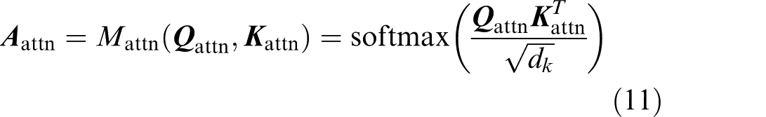
Contrary to many existing frameworks for intent or behaviour prediction, which can be modelled as classification problems, the aim of this research is to predict future positions for the TA across a prediction horizon, which is intrinsically a regression problem. The proposed model is shown in Figure 2.

Figure 2.

An LSTM-based encoder-decoder backbone is used to process the historical trajectories and generate the predictions. The SAs are identified by a range search and their historical trajectories, as well as that of the TA, are embedded by the LSTM. With these trajectory encodings, an AM-based Interaction encoder is used to mine interaction clues between the TA and SAs. The reachable map elements are abstracted by 1D convolution. The most likely map element that the TA will reach is identified by AM in the map element estimation module and the corresponding map feature encoding is extracted, as well as the encoding of AOI. Another AM-based goal point estimation module is then applied to fuse the scene context encodings, including the map and interaction encodings, and estimate the final goal. At last, LSTM is used to generate the final predictions with a concatenation of goal point encoding and the current state.

Trajectory encoder

The historical track of each agent (including the TA and SAs) is encoded by using an LSTM encoder. This module is widely applied in extracting features of sequential inputs.^37,38,40 At any time instant $t$ , a sequence of $h$ time steps of the trajectory history are passed through the encoder. The LSTM states for each agent are updated frame by frame over the $h$ past frames. The LSTM weights are shared across the sequences of all agents. The final LSTM state for each agent $i$ can be expected to encode the motion status of that agent. The sequential inputs are:

$${\mathit{D}}_i=\left[\begin{array}{cccc}{\mathit{D}}_i^{(t-h)},\hfill & \dots ,\hfill & {\mathit{D}}_i^{(t-1)},\hfill & {\mathit{D}}_i^{\left(t\right)}\hfill \end{array}\right].$$

(13)

At any time instant $t$ ,

$${\mathit{D}}_i^{\left(t\right)}=[{p_x}_i^{\left(t\right)},{p_y}_i^{\left(t\right)},{v_x}_i^{\left(t\right)},{v_y}_i^{\left(t\right)}],$$

(14)

$${\mathit{h}}_{\mathrm{hist}}^i,{\mathit{c}}_{\mathrm{hist}}^i=\mathrm{LSTM}({\mathit{D}}_i,({\mathit{h}}_{\mathrm{hidden}},{\mathit{h}}_{\mathrm{cell}})),$$

(15)

where ${\mathit{h}}_{\mathrm{hist}}^i$ and ${\mathit{c}}_{\mathrm{hist}}^i$ are the final hidden state and cell state of the LSTM, respectively. They have the same shape with a hidden size of $D_{\mathrm{LSTM}}$ . ${\mathit{h}}_{\mathrm{hidden}}$ and ${\mathit{h}}_{\mathrm{cell}}$ are the initialisation value of the LSTM hidden and cell states, which are vectors of zeros. In the equation, $i$ is the index of the agents where 0 for the TA and positive integers for SAs.

In the neighbour interaction encoder, self-attention will be used to mine interaction information among the TA and SAs, as shown in Section ‘Neighbour interaction encoder’. To keep the consistency, the same LSTM encoder is shared among the TA and SAs.

Neighbour interaction encoder

AM is used to mine the interaction between the TA and SAs. Self-attention is used; thus, the target and source matrices are designed to be the same and to include historical encodings of both the TA and SAs. In this case, the TA learns not only from the SAs’ encoding but also from itself. ⁴¹ Besides, the interaction among SAs could also be learned.

The agent interaction attention context is represented by:

$${\mathit{H}}_{\mathrm{nbr}}=\mathrm{Attn}({\mathit{H}}_{\mathrm{hist}}{\mathit{W}}_{\mathrm{hist}}^Q,{\mathit{H}}_{\mathrm{hist}}{\mathit{W}}_{\mathrm{hist}}^K,{\mathit{H}}_{\mathrm{hist}}{\mathit{W}}_{\mathrm{hist}}^V),$$

(16)

where ${\mathit{H}}_{\mathrm{nbr}}$ is the generated agent-agent attention context with a length of $n+1$ , ${\mathit{H}}_{\mathrm{hist}}$ is the aggregation of ${\mathit{h}}_{\mathrm{hist}}^i$ for both TA and SAs with a length of $n+1$ , and ${\mathit{W}}_{\mathrm{hist}}^Q$ , ${\mathit{W}}_{\mathrm{hist}}^K$ , and ${\mathit{W}}_{\mathrm{hist}}^V$ are learnable parameters performing linear projection.

TA’s encoding is appended after the aggregation of SAs’ encodings; thus the last element of ${\mathit{H}}_{\mathrm{nbr}}$ corresponds to the TA’s encoding fused with neighbour interaction context, denoted as ${\mathit{h}}_{\mathrm{nbrCtx}}$ .

In the source matrix, the neighbours are stored in a position-invariant way and their orders will not influence the attention results. To avoid training instability, encodings of zeros in the source matrix are used when SAs are absent.

Map element feature encoder

The map element feature encoder aims to extract geometry information, such as curvature, length and direction, by processing the original map element centre points.

A group of 1D convolution (1D Conv) layers and max-pooling layers are used to produce an implicit representation of the map element features. 1D Conv is usually used in encoding sequential data, such as past trajectories of agents^18,19 and ordered lane points, ¹⁷ and is also reported as efficient and lightweight. The map element feature encoder is illustrated in Figure 3. A group of 1D Conv and max pooling layers are shared among all map elements. By this map element feature encoder, the presentation of each map element is converted from a sequence of centrepoints to an array of high-dimensional features.

Figure 3.

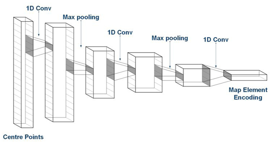
The map element feature encoder. Three layers of 1D Conv and two layers of max pooling are used to convert the centre points’ coordinates to a high-dimensional map element encoding.

The input is the map element feature matrix ${\mathit{M}}_{\mathrm{cnl}}$ with shape $(m,D_{\mathrm{pos}},n_{\mathrm{cpt}})$ , where $m$ denotes the number of map elements, $D_{\mathrm{pos}}$ denotes the dimension of centre point features ( $x$ and $y$ coordinates), and is the number of centre points in a single map element, which is 18 in this research.

The map element features are computed as:

$${\mathit{M}}_{\mathrm{conv}\mathrm{\_}1}=\mathrm{maxPl}\left(\mathrm{Conv}\mathrm{\_}1\left({\mathit{M}}_{\mathrm{cnl}}\right)\right),$$

(17)

$${\mathit{M}}_{\mathrm{conv}\mathrm{\_}2}=\mathrm{maxPl}\left(\mathrm{Conv}\mathrm{\_}2\left({\mathit{M}}_{\mathrm{conv}\mathrm{\_}1}\right)\right),$$

(18)

$${\mathit{M}}_{\mathrm{sce}}=\mathrm{Conv}\mathrm{\_}3\left({\mathit{M}}_{\mathrm{conv}\mathrm{\_}2}\right),$$

(19)

where $\mathrm{Conv}\_i\in \{1,2,3\}$ denotes 1D convolution layers and $\mathrm{maxPl}(·)$ represents the max pooling operation. Each 1D Conv layer uses a kernel size of 3, followed by a max-pooling layer with a kernel size of 2. All 1D Conv layers are followed by Leaky ReLU activation, omitted from equations for brevity. In addition, no padding is used in 1D Conv layers. Shapes of map element features after each layer are summarised in Table 2 below, which is also aligned with the illustration in Figure 3.

Table 2.

Shape of outputs after each layer in the map element feature encoder.

Layers	Shape of output
Input	$(m,2,18)$
1D Conv_1	$(m,D_{\mathrm{conv}\mathrm{\_}1},18)$
Max Pooling	$(m,D_{\mathrm{conv}\mathrm{\_}1},8)$
1D Conv_2	$(m,D_{\mathrm{conv}\mathrm{\_}2},6)$
Max Pooling	$(m,D_{\mathrm{conv}\mathrm{\_}2},3)$
1D Conv_3	$(m,D_{\mathrm{conv}\mathrm{\_}2},1)$

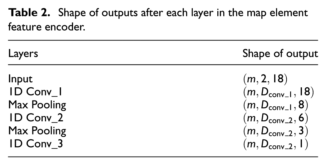
In Table 2, $D_{\mathrm{conv}\mathrm{\_}1}$ , $D_{\mathrm{conv}\mathrm{\_}2}$ and $D_{\mathrm{conv}\mathrm{\_}3}$ stand for channel dimensions of three 1D Conv layers, respectively.

Most likely map element estimator

The most likely (ML) map element to cover the final point of the trajectory is selected based on the co-relationship calculated by the TA’s historical encoding and map element feature encodings through cross-attention. This is inspired by LAformer, ²³ while the scene representation and module details are different. Rather than just generating a comprehensive map-aware encoding, the attention scores between the TA and map elements are first computed.

The map element selection is jointly determined by historical status and interactions with SAs. Practically, the TA’s historical encoding is first concatenated with the neighbour interaction encoding:

$${\mathit{h}}_{\mathrm{mQ}}=\mathrm{cat}({\mathit{h}}_{\mathrm{hist}}^0,{\mathit{h}}_{\mathrm{nbrCtx}}),$$

(20)

This joint encoding serves as the query vector, with the key-value pairs derived from map element feature encodings. The agent-map attention context is formulated as:

$${\mathit{A}}_{\mathrm{attnM}}=\mathrm{Attn}({\mathit{h}}_{\mathrm{mQ}}{\mathit{W}}_{\mathrm{map}}^Q,{\mathit{M}}_{\mathrm{sce}}{\mathit{W}}_{\mathrm{map}}^K),$$

(21)

where ${\mathit{W}}_{\mathrm{map}}^Q$ and ${\mathit{W}}_{\mathrm{map}}^K$ are learnable parameters performing linear projection.

The map element with the highest attention score is selected as the most likely map element and its map element encoding is therefore extracted, denoted as ${\mathit{M}}_{\mathrm{sce}}^{\mathrm{ML}}$ , for goal point estimation (seen in Section ‘Goal point estimator’).

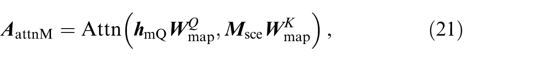
Additionally, a comprehensive context is derived from the AOI through:

$${\mathit{h}}_{\mathrm{AOI}}={\mathit{A}}_{\mathrm{attnM}}·{\mathit{M}}_{\mathrm{sce}}{\mathit{W}}_{\mathrm{map}}^V,$$

(22)

where ${\mathit{W}}_{\mathrm{map}}^V$ represents the learnable parameters for linear projection to generate value vectors and ${\mathit{h}}_{\mathrm{AOI}}$ denotes a fused encoding integrating map element features within the AOI, with a hidden size of $D_{\mathrm{mapAttn}}$ .

Map element features from all scenarios are aggregated into ${\mathit{M}}_{\mathrm{sce}}$ . Without distinguishing map elements across scenarios or considering reachability, the TA may inappropriately reference all elements in the container to compute weights, potentially misleading learning and causing ambiguity for DL-based models. Additionally, cBFS can identify insufficient map elements in the AOI due to edge cases, for example, at the margin of the map. To handle these cases, a dynamic map mask is introduced.

In detail, features of map elements within the AOI, explored via cBFS, are extracted from ${\mathit{M}}_{\mathrm{sce}}$ and are stored in ${\mathit{M}}_{\mathrm{sce}\mathrm{\_}\mathrm{AOI}}$ . Let $m_{\mathrm{AOI}}$ denote the maximum number of map elements allowed in the AOI. If fewer than $m_{\mathrm{AOI}}$ elements are extracted via cBFS, dummy map elements of zero-value features are appended to ensure matrix completeness of ${\mathit{M}}_{\mathrm{sce}\mathrm{\_}\mathrm{AOI}}$ . A local mask is then created to flag these dummy map elements in AOI:

$$\mathit{Mas}{\mathit{k}}_{\mathrm{AOI}}\left[i\right]\in {\{0,1\}}^{1\times m_{\mathrm{AOI}}}.$$

(23)

where $\mathit{Mas}{\mathit{k}}_{\mathrm{AOI}}$ assigns 1 to all dummy elements. Based on experimental validation, $m_{\mathrm{AOI}}$ is set to be 40 to balance data coverage and computational efficiency.

During the attention process in equation (21), logits for map elements in AOI are computed via the dot product. Prior to Softmax normalisation, logits corresponding to masked map elements are set to a negligible constant, for example, −9e15, ensuring their probabilities effectively become zero after Softmax, thus restricting selection to valid AOI elements.

For edge cases where no valid AOI elements are detected, the dummy element’s logit is set to a large value (e.g., 100). This forces the dummy element to receive a score of 1 with all others scoring 0, resolving ambiguity. This is particularly useful for cases like bicycles that may not adhere to lane structures and no map elements are matched, which has been neglected by published works based on Argoverse since only vehicles’ trajectories are predicted. Practically, bicycle map element encodings are zero-padded, as they often operate outside predefined road structures. Our approach can identify these cases and predict a trajectory accordingly.

Goal point estimator

The potential goal point of the prediction is closely related to scene context, which includes both map information ( ${\mathit{h}}_{\mathrm{AOI}}$ , ${\mathit{M}}_{\mathrm{sce}}^{\mathrm{ML}}$ ) and interactions between neighbouring agents ( ${\mathit{h}}_{\mathrm{nbrCtx}}$ ). To fuse these two context sources, they are aggregated into a single matrix to form an integrated context representation ${\mathit{H}}_{\mathrm{sce}}$ . Subsequently, an additional AM is employed:

$${\mathit{h}}_{\mathrm{endpt}}=\mathrm{Attn}({\mathit{h}}_{\mathrm{hist}}{\mathit{W}}_{\mathrm{sce}}^Q,{\mathit{H}}_{\mathrm{sce}}{\mathit{W}}_{\mathrm{sce}}^K,{\mathit{H}}_{\mathrm{sce}}{\mathit{W}}_{\mathrm{sce}}^V),$$

(24)

where ${\mathit{W}}_{\mathrm{sce}}^Q$ , ${\mathit{W}}_{\mathrm{sce}}^K$ and ${\mathit{W}}_{\mathrm{sce}}^V$ are learnable parameters performing linear projection. The resulting ${\mathit{h}}_{\mathrm{endpt}}$ can be interpreted as an endpoint encoding that integrates both map information and neighbouring interaction cues, with a hidden size of $D_{\mathrm{goalAttn}}$ .

By grounding goals in interpretable map elements, misguidance from over-reliance on single-lane centreline data can be avoided, and coarse learning from sets of less relevant scenario contexts can be prevented.

Finally, one FC layer is used to map the high-dimensional features to the goal point coordinates ${\mathit{P}}_{\mathrm{goal}}$ :

$${\mathit{P}}_{\mathrm{goal}}=\mathrm{FC}(\mathrm{cat}({\mathit{h}}_{\mathrm{hist}}^0,{\mathit{h}}_{\mathrm{endpt}})).$$

(25)

Trajectory decoder

An LSTM decoder is used to generate the future trajectories of the TA. At any time $t$ , the decoder generates the future trajectories over the subsequent $f$ time steps. At each prediction time step, the inputs comprise ${\mathit{D}}_0^{\left(0\right)}$ and ${\mathit{h}}_{\mathrm{endpt}}$ , and the hidden and cell states of the LSTM in the decoder are initialised by the outputs of the trajectory encoder:

$${\mathit{h}}_{\mathrm{pred}}^t,{\mathit{c}}_{\mathrm{pred}}^t=\mathrm{LSTM}(\mathrm{cat}({\mathit{D}}_0^{\left(0\right)},{\mathit{h}}_{\mathrm{endpt}}),({\mathit{h}}_{\mathrm{hist}}^0,{\mathit{c}}_{\mathrm{hist}}^0)).$$

(26)

Then the MLP is used to output the deterministic coordinate at time $t$ :

$${\hat{\mathit{Y}}}^{\left(t\right)}=\mathrm{MLP}\left({\mathit{h}}_{\mathrm{pred}}^t\right).$$

(27)

Notably, the estimated goal point coordinate ${\mathit{P}}_{\mathrm{goal}}$ is excluded from the input of the LSTM decoder; instead, ${\mathit{h}}_{\mathrm{endpt}}$ is used for its richer contextual information compared to a 2D coordinate. However, ${\mathit{P}}_{\mathrm{goal}}$ is incorporated into the loss function to guide model training.

Training loss function

In the prediction structure, two intermediate outputs are generated: the most likely reachable map element and the potential goal point. These two outputs are highly related to the manoeuvre intention and an accuracy prediction improves the explanability of the prediction model. Thus, a comprehensive loss function is established to evaluate these two outputs, as well as the overall trajectory prediction accuracy.

The mean square error (MSE) is used to calculate the regression loss of trajectory points during training:

$$\mathrm{MSE}=\frac{1}{p}\sum _{i=1}^p[{(x_{t+i}-x_{t+i}^{\mathrm{gt}})}^2+{(y_{t+i}-y_{t+i}^{\mathrm{gt}})}^2].$$

(28)

The goal point estimation loss is calculated as the deviation from the goal estimation to its ground truth:

$$S{E}_{\mathrm{goal}}=[{(x_{\mathrm{goal}}-x_{t+p}^{\mathrm{gt}})}^2+{(y_{\mathrm{goal}}-y_{t+p}^{\mathrm{gt}})}^2].$$

(29)

The map element matching is a classification task. The negative log-likelihood (NLL) loss is used to calculate the matching loss:

$$\mathrm{NL}{L}_{\mathrm{map}}=-{\log }_2(\sum _{i=0}^m{\mathit{A}}_{\mathrm{attn}}^i·{\mathit{Mask}}_{\mathrm{map}\mathrm{\_}\mathrm{gt}}^i),$$

(30)

where $\mathit{Mas}{\mathit{k}}_{\mathrm{map}\mathrm{\_}\mathrm{gt}}$ is an array of binary values and the ground truth is set to be one and others zero.

To address the spatial overlap issue of map elements in intersection and roundabout scenarios, a matching algorithm based on trajectory-complete lane similarity is used to accurately associate trajectory points with map elements by identifying the target driving lane. Since the prediction of bicycles does not rely on map elements, for a fair comparison, the NLL excludes the results of map element matching of bicycles.

The final loss function during training is as follows:

$$\mathrm{loss}=\alpha \mathrm{MSE}+\beta S{E}_{\mathrm{goal}}+\gamma \mathrm{NL}{L}_{\mathrm{map}},$$

(31)

where $\alpha =1$ , $\beta =1$ and $\gamma =1$ to match the scale of these three costs into the same order of magnitude.

Experiment evaluation

Numerical experiments have been conducted on the inD dataset ³³ and the rounD dataset. ³⁴ The inD dataset contains four unsignalised intersections and three of them (Bendplatz, Heckstrasse and Neukoellner) are used in this research, including one four-arm intersection and two T-junctions. One additional roundabout from the rounD dataset is selected to supplement samples with varying RLs and TA dynamics.

Data description

Agent data are split into training, validation and testing sets. To minimise the imbalance of the manoeuvre patterns (going through, turning left and turning right), data samples are split according to agent types and manoeuvre patterns. More specifically, with a selected agent type and a chosen manoeuvre, 80% of agent data are sliced into the training set, 10% to the validation set and 10% to the testing set. This configuration is similar to those used in works of Geng et al.^42,43 Detailed statistics of samples are shown in Table 3.

Table 3.

Statistics of samples extracted from the inD and rounD datasets.

Agent Class	Mnvr	Intxn A			Intxn B			Intxn C			Intxn D
		Trng	Valid	Tstg	Trng	Valid	Tstg	Trng	Valid	Tstg	Trng	Valid	Tstg
Cars	GTH	536	67	67	436	55	56	1106	138	138	72	9	9
	TL	372	47	48	87	11	12	136	17	17	17	3	2
	TR	310	39	40	80	10	11	178	22	23	21	3	2
Trucks	GTH	22	2	3	11	1	2	45	6	7	23	3	3
	TL	3	0	1	7	1	1	28	3	4	3	1	1
	TR	4	0	1	8	1	1	38	5	5	4	1	1
Bicycles	GTH	201	25	25	17	2	3	23	3	4	1	0	1
	TL	65	8	8	1	1	1	7	1	3	0	0	0
	TR	59	7	8	2	1	1	8	2	2	0	0	0
Overall		1572	195	201	649	83	88	1569	197	203	141	20	17

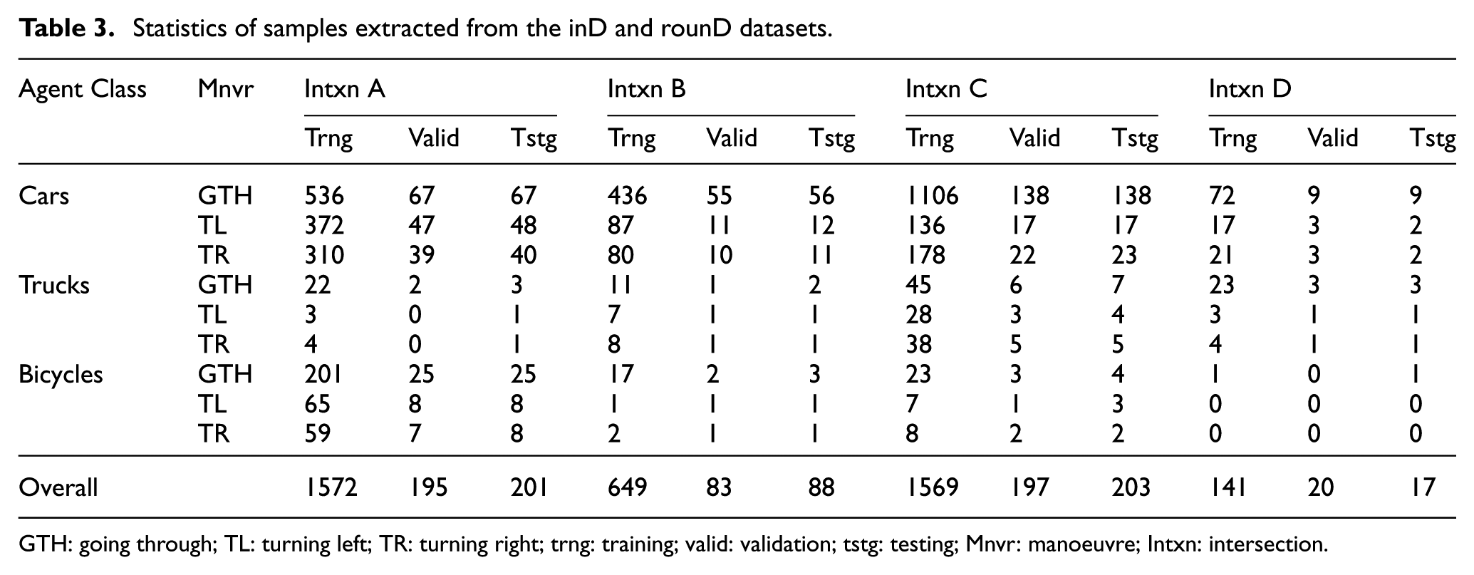
GTH: going through; TL: turning left; TR: turning right; trng: training; valid: validation; tstg: testing; Mnvr: manoeuvre; Intxn: intersection.

Evaluation metrics

Two widely used measures of prediction effectiveness are employed for performance evaluation. Lower values indicate better prediction performance.

Final Displacement Error (FDE) ⁴⁴ : This metric calculates the L2 distance between the predicted trajectory endpoint and the ground truth endpoint:

$$\mathrm{FDE}=\frac{\sum _{i=1}^N\sqrt{{(x_{t+p}-x_{t+p}^{\mathrm{gt}})}^2+{(y_{t+p}-y_{t+p}^{\mathrm{gt}})}^2}}{N},$$

(32)

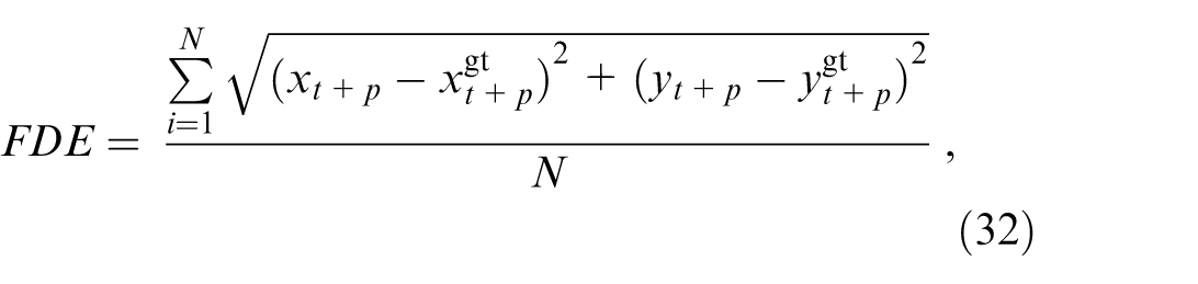
where $x_{t+p}$ and $y_{t+p}$ represent the predicted 2D position coordinates of a TA at the last time step $t+f$ of the prediction horizon. The superscript $\mathrm{gt}$ represents that the data are from the ground truth; otherwise, from the prediction.

The final trajectory prediction point is related to the TA’s driving intention, so it is important to evaluate its accuracy. ⁴⁴

Average Displacement Error (ADE) ⁴⁴ : It is used to measure the overall distance deviation of the predicted trajectory to the ground truth:

$$\mathrm{ADE}=\frac{\sum _{i=1}^N\sum _{t=1}^p\sqrt{{(x_{t+i}-x_{t+i}^{\mathrm{gt}})}^2+{(y_{t+i}-y_{t+i}^{\mathrm{gt}})}^2}}{N·p},$$

(33)

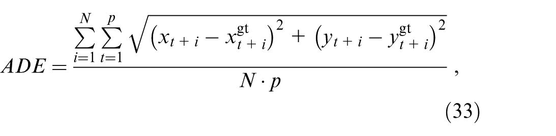
where $x_{t+i}$ , $y_{t+i}$ represent the predicted trajectory point at the timestep $t+i$ .

Implementation details

In this research, the prediction model is aimed at performing trajectory prediction up to 4 s with an observation of the past 2 s, denoted as $t_{\mathrm{pred}}$ and $t_{\mathrm{hist}}$ respectively. The data in the inD are recorded at 25 Hz. For training purposes, these data are down-sampled to 5 Hz, resulting in a length of 11 in the historical data and a length of 20 in the prediction.

The model is implemented using PyTorch. In the model training, Adam is used as the optimiser, with a batch size of 128 and an initial learning rate of 0.001, respectively. The proposed method is trained for 40 epochs, and the learning rate is multiplied by 0.7 every 8 epochs. To reduce the overfitting, the dropout rate is set to be 0.3. The training is deployed on the Nvidia GPU A100 within a High-Performance-Computing (HPC) platform.

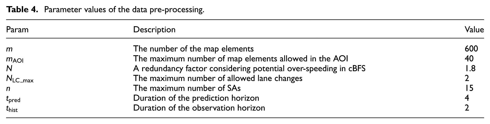
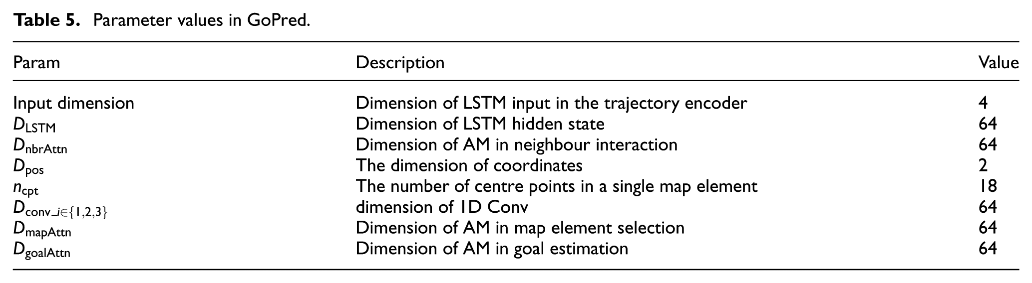
The general settings and the dimensions of layers in key modules are represented in Tables 4 and 5.

Table 4.

Parameter values of the data pre-processing.

Param	Description	Value
$m$	The number of the map elements	600
$m_{\mathrm{AOI}}$	The maximum number of map elements allowed in the AOI	40
$N$	A redundancy factor considering potential over-speeding in cBFS	1.8
$N_{\mathrm{LC}\mathrm{\_}\max }$	The maximum number of allowed lane changes	2
$n$	The maximum number of SAs	15
$t_{\mathrm{pred}}$	Duration of the prediction horizon	4
$t_{\mathrm{hist}}$	Duration of the observation horizon	2

Table 5.

Parameter values in GoPred.

Param	Description	Value
Input dimension	Dimension of LSTM input in the trajectory encoder	4
$D_{\mathrm{LSTM}}$	Dimension of LSTM hidden state	64
$D_{\mathrm{nbrAttn}}$	Dimension of AM in neighbour interaction	64
$D_{\mathrm{pos}}$	The dimension of coordinates	2
$n_{\mathrm{cpt}}$	The number of centre points in a single map element	18
$D_{\mathrm{conv}\mathrm{\_}i\in \{1,2,3\}}$	dimension of 1D Conv	64
$D_{\mathrm{mapAttn}}$	Dimension of AM in map element selection	64
$D_{\mathrm{goalAttn}}$	Dimension of AM in goal estimation	64

Results of cBFS

The cBFS produces a set of potential destination map elements and the top-K hit rates, which indicate positional identification of ground truth map elements within the top K results, are used for performance evaluation. The higher the hit rate is, the better the performance of exploration. Besides, missing rates (MR) are used for evaluation, which stand for the proportion of destination map elements unidentified in the search results. Alongside the proposed cBFS, DFS and intuitive range searching (RngS) are evaluated, given that they are widely used in applications.^8,29,45 In the performance analysis, the maximum number of stored map elements is set to 90 to show the complete searching results of the algorithms, while it is set to 40 in the DL application for lightweight storage. The cBFS and DFS search reachable map elements along the RL while the RngS collects the map elements within a radius in a homogeneous way.

In equation (7), a redundancy factor $N$ should be pre-defined prior to conducting cBFS. To determine a reasonable value for $N$ , kernel density estimation (KDE) was performed to analyse the speed distributions of cars, buses, and bicycles. The resulting speed profiles are presented in Figure 4. To ensure coverage of 99.99% of real-world cases, $N$ in equation (7) is set to be 1.8.

Figure 4.

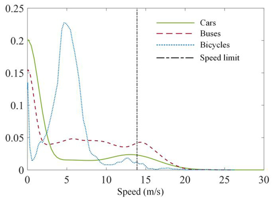
The speed distribution of cars, trucks and bicycles. The speed limit of the scenarios is 13.9 m/s and is marked as a black dash-dotted line. For all three traffic agents, there is a small peak near the speed limit, indicating that traffic agents tend to move around the speed limit. Besides, over-speeding cannot be ignored.

The second hyperparameter for cBFS is the maximum number of allowed lane changes, denoted as $N_{\mathrm{LC}\mathrm{\_}\max }$ . Performing multiple lane changes within a short timeframe, for example, 4 s, can degrade ride comfort, increase driver workload and lead to a manoeuvre deviating from normal driving conditions.

To investigate the feasibility of such manoeuvres within the prediction horizon, simulations were conducted in CarSim. The speed range is set to 20 to 60 km/h, aligning with urban driving scenarios. Within a 4 s trajectory prediction horizon, a single lane change involves a lateral displacement of 3.5 m, a distance matching the typical width of driving lanes as referenced in literature. ⁴⁶ Individual lane change paths are generated using quintic polynomial curves to ensure smooth transitions between lane centres during constant velocity travel. Results for lateral acceleration $a_{\mathrm{lat}}$ and yaw rate $\omega$ are summarised in Table 6.

Table 6.

Simulation results of vehicle dynamics under multiple lane changes.

Numberof lanechanges	Speed(km/h)	Extreme values		Final states at 4 s
		$a_{\mathrm{lat}}$ (m/s2)	$\omega$ (°/s)	$a_{\mathrm{lat}}$ (m/s2)	$\omega$ (°/s)
1	20	0.082	8.080	0.051	6.771
	30	0.110	7.372	0.043	4.466
	40	0.123	6.247	0.033	2.787
	50	0.126	5.160	0.031	1.871
	60	0.130	4.371	0.028	1.196
2	20	0.181	17.967	0.156	17.534
	30	0.222	14.233	0.111	10.350
	40	0.248	12.252	0.089	6.663
	50	0.255	10.207	0.080	3.394
	60	0.259	8.682	0.069	2.789
3	20	0.252	23.394	0.277	23.078
	30	0.316	20.275	0.230	18.217
	40	0.361	17.885	0.194	12.416
	50	0.377	15.150	0.166	8.254
	60	0.384	12.971	0.136	5.236

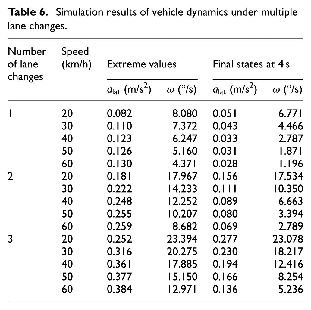
Lateral acceleration and yaw rate are key indicators of ride comfort and manoeuvre stability. Simulation results reveal critical dynamics limitations associated with increasing lane change number within 4 s. At low speeds (≤30 km/h), 2 to 3 consecutive lane changes produce yaw rates exceeding 15 °/s, such as 17.967 °/s for 2 lane changes at 20 km/h and 20.275 °/s for 3 lane changes at 30 km/h. These yaw rate values far surpass the 8 °/s threshold observed in naturalistic driving with an average value of 1.4 °/s, ⁴⁷ indicating aggressive manoeuvring inconsistent with human driving norms. At higher speeds (≥50 km/h), lateral acceleration becomes the constraining factor. For instance, the 3-lane-change mobility at 50 km/h generates peak lateral acceleration of 0.377 g and large yaw rates of 15.15 °/s, approaching the 0.4 g comfort limit defined by Bosetti et al. ⁴⁷ and surpassing the naturalistic driving threshold of 8 °/s. Notably, final states at 4 s show non-zero yaw rates and lateral accelerations for 3-lane changes, for example, 8.25 °/s and 0.166 g at 50 km/h, confirming incomplete manoeuvre execution within the defined prediction horizon. In contrast, two-lane changes maintained lateral acceleration below 0.3 g across all speeds and had final states with smaller residual dynamics.

Theoretical justification for the two-lane change constraint is further reinforced by scenario behavioural statistics. In the analysis, a lane change manoeuvre is defined as the TA transitions to either a direct neighbour of its current lane segment or a successor of the direct neighbour of its current lane segment, as shown in Figure 5.

Figure 5.

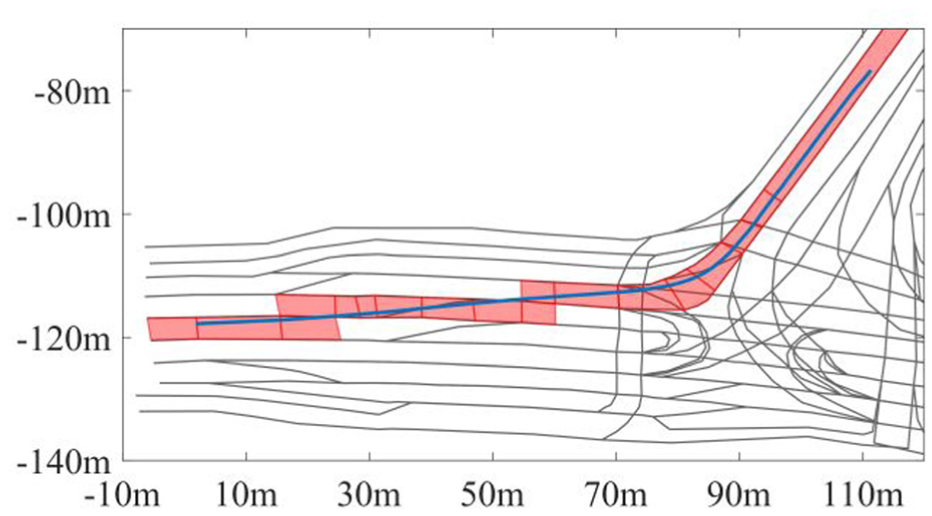
An example of an agent executing two lane changes in Intxn C. The trajectory direction is from right to left.

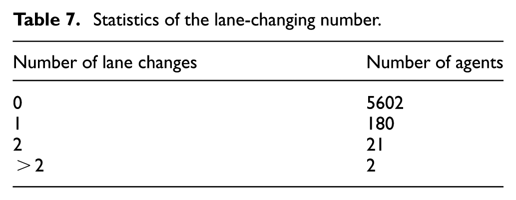
Note that there are edge cases that travel across the road to perform a parking manoeuvre. They perform more than two lane changes within the prediction horizon. These cases are excluded from the dataset, as they fall outside the scope of the target prediction manoeuvres. The statistics of lane-changing numbers are provided in Table 7.

Table 7.

Statistics of the lane-changing number.

Number of lane changes	Number of agents
0	5602
1	180
2	21
>2	2

Based on the analysis of lane-changing manoeuvres of cars and trucks in the inD dataset and the simulation results based on Carism, $N_{\mathrm{LC}\mathrm{\_}\max }$ is set to be 2, considering the feasible number of lane changes within the prediction horizon of 4 s.

The results of the top 40 hit rates are shown in Table 8. Across all scenarios, cBFS demonstrates balanced performance characteristics. In Intxn A, cBFS achieves a hit rate reaching 0.996 at the top 40 elements with the minimal MR of 0.003, outperforming both DFS and RngS. DFS exhibits strong initial performance with 0.926 at the top 10 elements, but plateaus at 0.928. This is because DFS searches with a deep depth before switching to another direction. Though this is aligned with the truth that vehicles keep going straight most of the time due to the simplicity of the intersection arm topology, it fails to identify destination map elements promptly due to lane changing. In Intxn B, cBFS maintains 0.998 hit rates at the top 40 elements with a negligible MR of 0.001. In a more complex scenario, like Intxn C, where more lanes exist in one driving direction, LC actions exist with a higher possibility. This scenario highlights cBFS’s performance, achieving a top 40 hit rate of 0.965 while DFS only achieves 0.922. Intxn D further demonstrates cBFS adaptability to road topology variation like roundabouts, where it reaches 0.996 hit rates by the top 20 elements, outperforming DFS delayed convergence. In all four scenarios, the performance of RngS varies a lot, with top 40 hit rates ranging from 0.439 to 0.871. This is because it cannot extend along the lane direction and includes too many map elements in the lane traversal directions, demonstrating poor adaptability to road layout variance.

Table 8.

The results of the top-K hit rate.

		Top-K Hit Rate				MR(Top 90)
		5	10	20	40
Intxn A	RngS	0.462	0.605	0.691	0.743	0.070
	DFS	0.823	0.926	0.927	0.928	0.050
	cBFS	0.867	0.933	0.983	0.996	0.003
Intxn B	RngS	0.504	0.594	0.656	0.732	0.142
	DFS	0.679	0.780	0.915	0.930	0.001
	cBFS	0.684	0.785	0.921	0.998	0.001
Intxn C	RngS	0.213	0.291	0.356	0.439	0.372
	DFS	0.438	0.692	0.788	0.922	0.033
	cBFS	0.481	0.686	0.855	0.965	0.022
Intxn D	RngS	0.217	0.274	0.510	0.871	0
	DFS	0.598	0.771	0.782	0.996	0.004
	cBFS	0.492	0.885	0.996	0.996	0.004

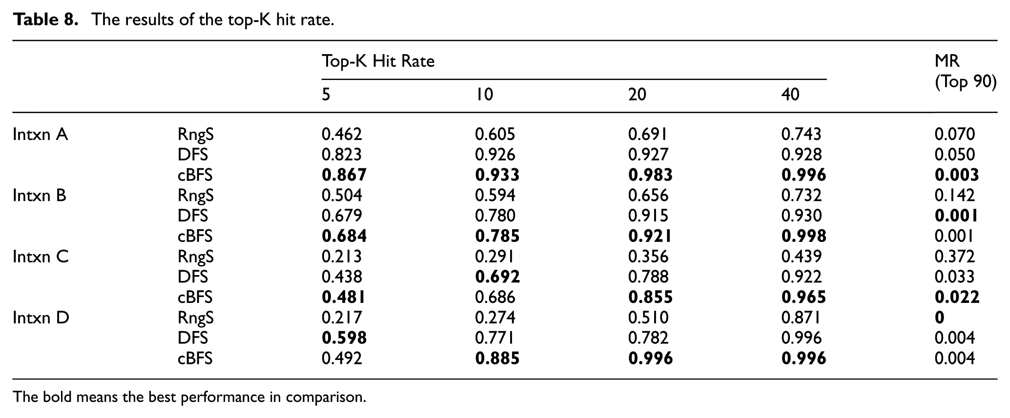
The bold means the best performance in comparison.

The detailed distributions of ranking hit rates at Intxn C and Intxn D are illustrated in Figure 6(a) and (b), respectively. The results reveal that DFS identifies ground truth map elements earlier in rankings but struggles with topological variations. As Figure 6(b) shows, DFS’s unidirectional deep search fails to detect the ground truth destination in early stages in the multi-entrance and multi-exit roundabout, with a secondary hit rate peak around position 25. In comparison, through searching on the longitudinal and lateral directions consecutively, cBFS can successfully identify ground truth during forward exploration and produces a more fluent ranking hit rate distribution. Additionally, RngS consistently shows dispersed hit rate distributions with delayed peaks, confirming its unoriented search mechanism inefficiency.

Figure 6.

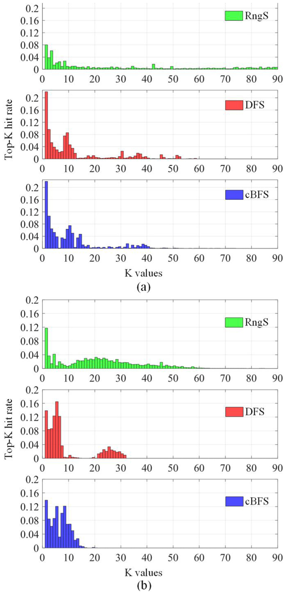
The top 90 ranking hit rate distributions at Intxn C and D are illustrated in (a) and (b), respectively.

In terms of time efficiency, cBFS, DFS, and RngS require 113.0 s, 106.6 s, and 430.6 s, respectively, to complete AOI exploration across all four scenarios on a device equipped with an Intel Core i7-8700K CPU and 24 GB of memory. cBFS is efficient and exhibits performance comparable to DFS. Although RngS is theoretically efficient due to its unidirectional search mechanism, it performs 3,880,200 operations, substantially more than the 73,216 operations of both cBFS and DFS. The large number of operations for RngS arises because it searches the AOI trajectory on a point-by-point basis, whereas cBFS and DFS perform exploration processing only when occupied map elements change between consecutive trajectory points.

Trajectory prediction results

To validate the efficacy of the proposed GoPred, it is compared to some representative models based on the data described in Section ‘Data description’. These include the vanilla LSTM, mCS-LSTM and GA-LSTM. The vanilla LSTM method uses an encoder-decoder structure, which is widely used and reported.^49,50 The encoder and decoder are set to be the same as those in Sections ‘Trajectory encoder’ and ‘Trajectory Decoder’ and they rely solely on TA’s historical status. mCS-LSTM is modified from CS-LSTM which encodes the neighbour interaction through convolutional social pooling (CSP). ² The manoeuvre probability module is eliminated from CS-LSTM since unimodal prediction is deployed in this work. GA-LSTM is a variation of the proposed method that shares most of the configuration. The neighbour interaction is encoded by AM, the same as GoPred, and the encoding of the estimated goal point is used to supplement the input of the decoder. The difference is that the interaction between the map and the TA is mined by a GCN. This GCN-based map mining module is inspired by the lane convolution operator laneGCN ³ and a stack of multi-scale GCNs are used. Specifically, aggregation steps of 1, 2, 4 and 8 are deployed respectively with the same configuration of GCN and the results of these individual aggregations are fused to generate the final map-aware encoding and to supplement the input of the goal point estimation. This multi-scale GCN is used to reach topologically far-side map elements.

To ensure fairness in comparison, the hidden sizes of all models are kept consistent. Refer to Table 5 for details. Each model is trained 10 times and the average performances are shown in Table 9. Metrics of ADE and FDE are calculated, alongside the number of learnable parameters (#Param), inference latency and giga floating-point operations (GFLOPs).

Table 9.

Prediction results.

	#Param	Latency(ms)	GFLOPs	ADE				FDE
				car	bus	bicycle	overall	car	bus	bicycle	overall
Vanilla LSTM	35,458	0.55	0.009	1.035	1.044	0.824	1.007	2.794	2.781	2.198	2.712
mCS-LSTM	114,962	1.43	0.024	0.890	0.906	0.723	0.868	2.296	2.264	1.846	2.233
GA-LSTM	159,748	25.11	0.042	0.817	0.838	0.624	0.792	2.203	2.192	1.580	2.117
GoPred	146,954	9.93	0.099	0.761	0.803	0.611	0.743	2.011	2.047	1.495	1.943

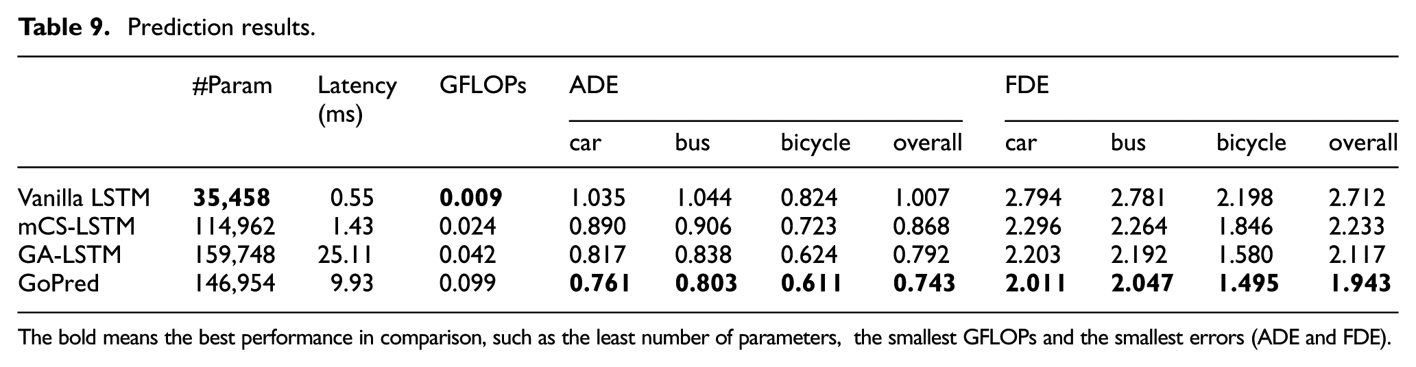
The bold means the best performance in comparison, such as the least number of parameters, the smallest GFLOPs and the smallest errors (ADE and FDE).

Overall, the proposed GoPred achieves better performance than the others in terms of ADE and FDE. Specifically, when information from the SAs and RL is fused, the ADE and FDE are reduced by 26.2% and 28.4% respectively, compared to the baseline vanilla LSTM.

As shown in the comparison of mCS-LSTM and vanilla LSTM, neighbour interaction can improve the prediction accuracy. Improvements of 13.8% and 17.7% on ADE and FDE are reported in the comparison. Further prediction error reduction is achieved by supplementing RL information, as shown in the results of GA-LSTM and GoPred. By comparison, the AM is better at mining the relation between the TA and RL information. The ADE and FDE are reduced by 6.2% and 8.2% when AM is used compared to GCN in GA-LSTM.

Figure 7 illustrates displacement error (DE) evolution over the prediction horizon. As expected, prediction errors exhibit a general upward trend with increasing horizon length. Notably, GA-LSTM outperforms GoPred marginally for prediction horizons under 2 seconds. This discrepancy can be attributed to their architectural differences. GCN-based RL mining strategy in GA-LSTM prioritises local map element interactions, for example, immediate predecessors and neighbours. Though the multi-step message propagation strategy can reach topologically distant lane segments, their features become blurred during aggregation. Feature degradation from distant nodes in GCN is inevitable, which makes GCN focus more on local RL information and thereby provide better prediction performance in the short horizon as TA typically does not travel far. In contrast, the focus of GoPred is on potential destination inference and therefore provides better long-horizon performance.

Figure 7.

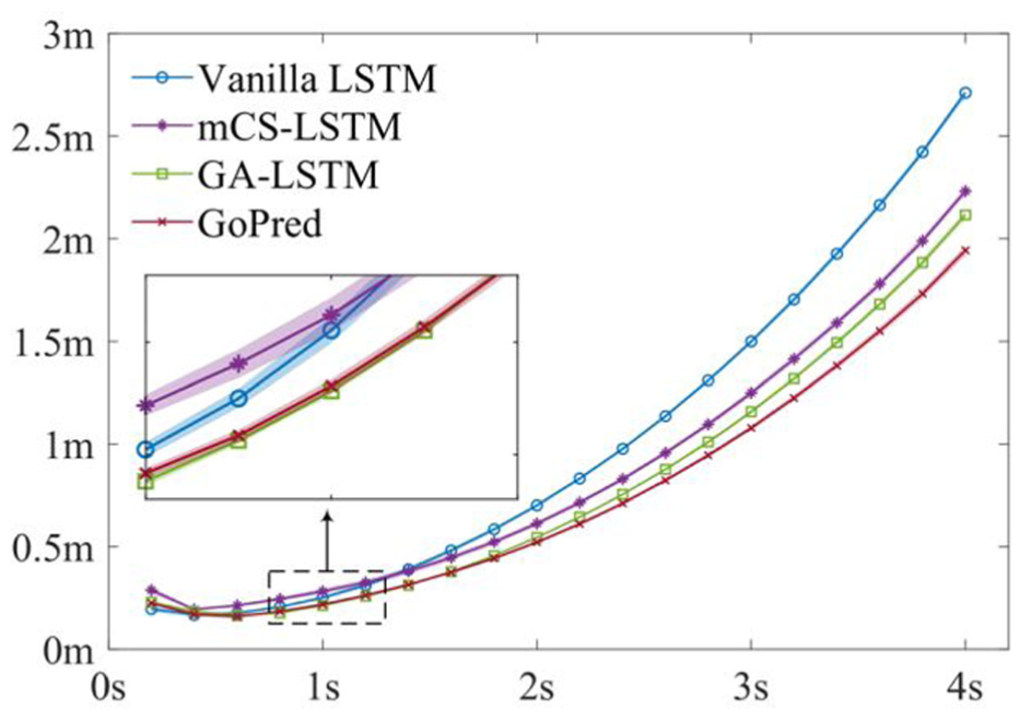
The DEs across the prediction accuracy. They increase with the growth of the prediction horizon. The minimum DE is not achieved at the closest prediction horizon (0.2 s) but at the second (0.4 s).

An observation is that the minimum DE does not occur at the shortest horizon (0.2 s), likely due to stop-and-go manoeuvres introducing noise in low-speed trajectory data, e.g., from inherent data drift in the original dataset. Despite such noise at low speeds, no additional filtering was applied, as predictions remained within acceptable accuracy thresholds.

GFLOPs were measured with a batch size of 16, mimicking the traffic scenario where 16 TAs are around the AV. ²⁹ This metric evaluates the computational complexity. In terms of computational efficiency, the vanilla LSTM achieves optimal performance, owing to its highly compact architecture that excludes additional neighbour or map interaction inputs. This minimal design results in a parameter size of 35.458 K. Conversely, GoPred exhibits the highest GFLOPs, as high as 0.098, with its computational overhead primarily attributed to the map element feature encoder and the downstream most likely map element estimator. The convolutional layers introduce a large number of learnable parameters, significantly increasing operational complexity and resulting in a 0.057 GFLOPs increment compared to GA-LSTM. Although GA-LSTM also incorporates RL processing, its computational demands remain moderate. Its GCN module processes RL data through MLPs and graph convolution operations, both of which feature low inherent complexity. While GA-LSTM demonstrates greater efficiency than GoPred, it exhibits limited long-term prediction performance.

Though having a higher complexity than other methods in this research, GoPred is still a lightweight model, compared to other dedicated models which normally have a parameter size larger than 200,000 and GFLOPs over 0.4. ²⁹

The inference latency of various models was evaluated on a single RTX 6000 GPU, with results presented in Table 9. Vanilla LSTM and mCS-LSTM demonstrate minimal latency at 0.55 ms and 1.43 ms, consistent with their low computational complexity and compact architecture. Notably, GoPred exhibits a latency of 9.93 ms despite its higher computational load of 0.099 GFLOPs. In contrast, GA-LSTM shows substantially elevated latency of 25.11 ms even with a lower theoretical complexity of 0.042 GFLOPs. This 15.18 ms difference between the two models presents a discrepancy that arises from the GCN-based map feature extraction module in GA-LSTM. This multi-layer component employs sparse matrix storage for graph adjacency representations, introducing inherent computational inefficiencies on GPU architectures. The sequential neighbourhood aggregation in GCN layers further increase latency by limiting parallelisation. In contrast, GoPred utilises compact storage by arranging key map elements within the AOI, minimising computations through focusing relevant map elements and executing efficient matrix operations.

The evaluation of map element estimation accuracy hinges on two metrics: per-rank hit rate and top-K (K = 5) hit rate. These metrics quantify the likelihood of the ground truth appearing at specific rank positions (first, second, …, fifth) and the probability that the ground truth is included in the top five predicted ranks, respectively.

As presented in Table 10, the estimation process successfully places the ground truth at the first rank with a 73.1% success rate. This result underscores a substantial degree of accuracy in initial guesses.

Table 10.

Per-rank hit rates of map element estimation.

First	Second	Third	Fourth	Fifth	top_5	w/ nbr
0.731	0.156	0.057	0.020	0.009	0.972	0.901

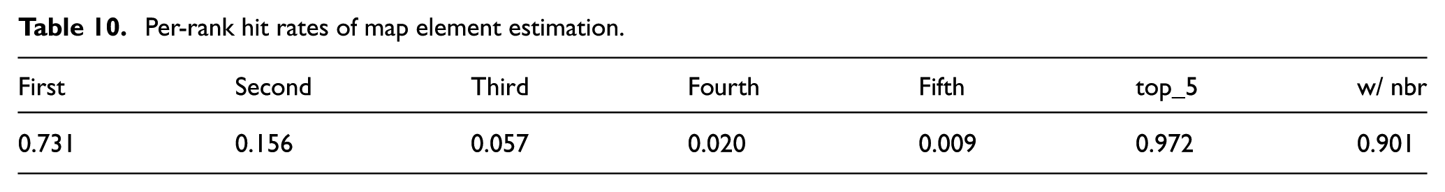
Though there is a notable decline in confidence from the first to the second rank, the top-5 hit rate remains high at 97.2%, indicating that a large majority of the ground truth elements are captured within the first five predictions. This reflects a broad enclosure of potential correct predictions.

An additional metric assesses the probability that the estimation aligns with either the first prediction or the direct neighbours of the first prediction, including the immediate successor, predecessor, right and left neighbours. The result is represented in the last column in Table 10. The value reaches 90.1%, indicating an accurate prediction. This metric is particularly critical for evaluating the map element estimation performance since it is vague to assign a deterministic map element to the TA while it is transitioning between two adjacent map elements.

To better demonstrate the prediction performance of the proposed method, the visualisation results of prediction at specific intersections are illustrated, as shown in Figure 8. As illustrated, the most likely map element estimator effectively identifies the most relevant map elements inside AOI. When the TA approaches the intersection, the estimator generates confidence scores for associated map elements, quantifying uncertainties in moving intentions. Notably, TA reaches the most probable map elements at the end of the prediction horizon, though not exactly, validating the module’s effectiveness. Furthermore, the goal point prediction is softly constrained by the most likely map element and shows alignment with the ground truth endpoint. Both the map element estimation and goal point prediction progressively reveal the TA's movement intentions, facilitating enhanced interpretability of the prediction model. The consistency between map element estimation and goal prediction further confirms the model's effectiveness in narrowing the inference space and inferring movement intentions.

Figure 8.

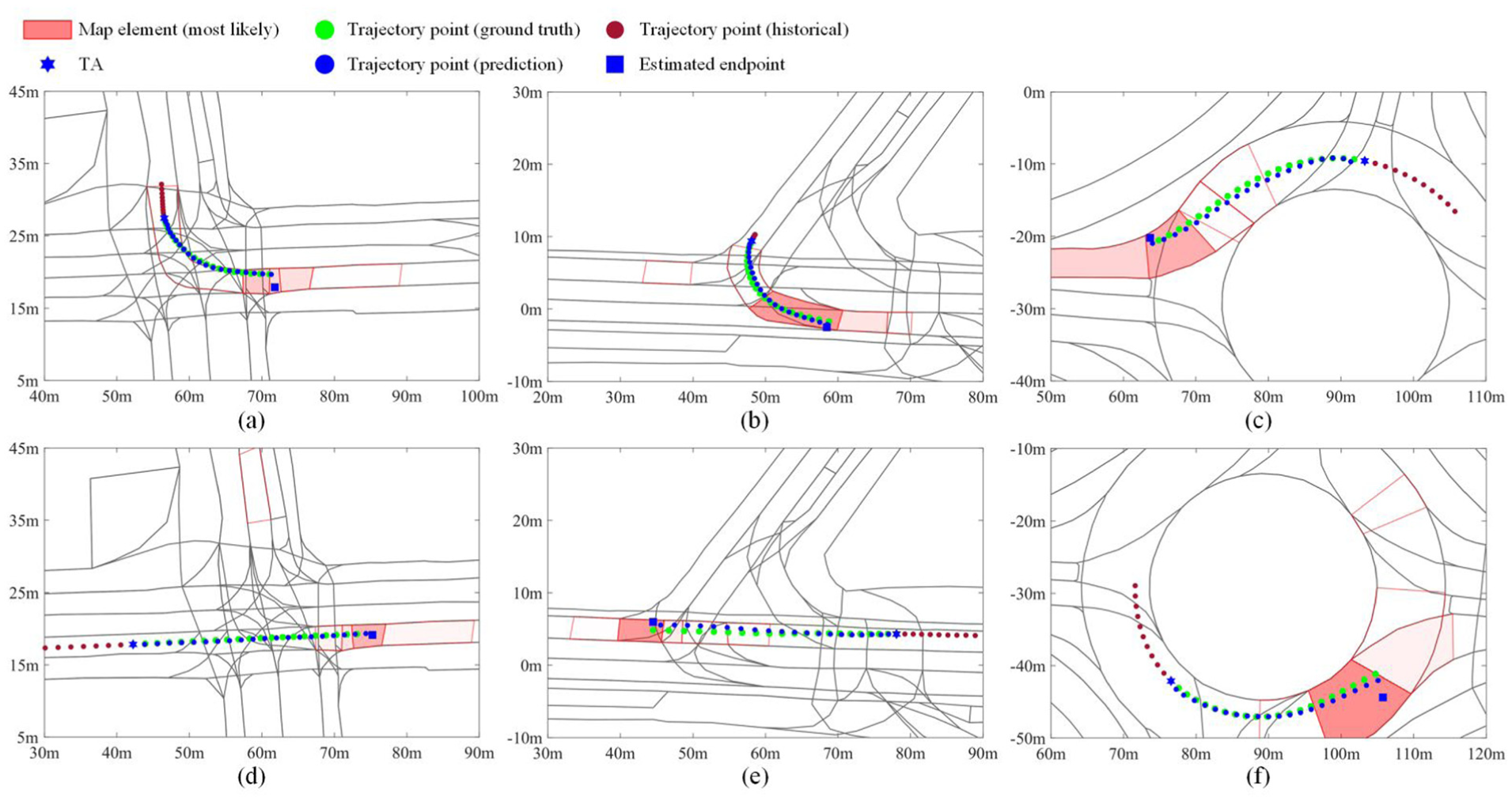
The prediction results of the proposed method. The top five most likely map elements are plotted in red with transparency. The higher the opacity, the higher the possibility. The estimated goal points are plotted as blue square markers. The waypoints of the historical trajectory, predicted trajectory and ground truth are represented by red, blue and green, respectively.

To provide a detailed illustration of how the prediction model estimates TA intention within intersections, a left turn case is selected, as shown in Figure 9. As the TA approaches the intersection, cBFS first identifies reachable map elements (Figure 9(a)), with initial most-likely map element predictions indicating a lane-keeping manoeuvre (Figure 9(d)). Upon nearing the intersection entrance, the TA decelerates to prepare for turning while avoiding collisions with SAs. At this stage, the estimated map elements suggest three potential manoeuvres: left U-turn, continuation to a proximal map element on the current lane or right lane change. Due to reduced speed, close side map elements are paid attention to.

Figure 9.

An example of TA executing a left-turn manoeuvre at the intersection. The top row demonstrates map elements inside AOI as grey polygons, with ground truth map elements highlighted in blue to represent the actual intention of the selected sample. The bottom row illustrates the trajectory prediction results. The waypoints of the historical trajectory, predicted trajectory and ground truth are represented by red, blue and green, respectively. Meanwhile, SAs are marked as red hexagons alongside their historical positions, providing context for the dynamic traffic environment around the TA.

As the TA enters the intersection, cBFS dynamically narrows the reachable map elements to those on the left-turn lane. Consequently, a high-confidence score is assigned to the left-turn lane map element, establishing a coarse-grained destination. Across all three sub-scenarios in Figure 9, corresponding goal points are predicted in alignment with the most likely map elements. These goal points not only align spatially with their associated map elements but also provide finer-grained localisation of the TA's intention, particularly valuable given the extended length of map elements.

Ablation experiments

This section investigates the significance of critical components in trajectory prediction models. GoPred progressively narrows the search space by exploring AOI and scoring corresponding map elements. It then generates a comprehensive goal encoding by integrating AOI encoding and neighbourhood interaction encoding, which further facilitates the prediction.

In GoPred, neighbour interaction encoding plays a vital role in estimating the most likely map elements and goal points. The estimated map elements help constrain potential goal generation and contribute to forming informative goal encodings. To further examine their impact on trajectory prediction, ablation experiments were conducted by removing relevant modules from the prediction backbone. Performance was evaluated using map element estimation accuracy, goal estimation deviation, ADE and FDE.

The ablation results show that the model with all modules in position achieved optimal ADE and FDE performance, as it simultaneously incorporates map information and neighbour interactions, as shown in Test 1 of Table 11. When map information was excluded, as shown in Test 2, the model relied on supplementary neighbour interactions to estimate potential goals. This omission increased goal prediction errors, leading to 13.7% and 12.3% rises in ADE and FDE, respectively. Excluding neighbour interactions caused the largest performance degradation. As shown in Test 3, first rank hit rate dropped by 3.1%, while ADE and FDE surged by 16.3% and 19.2%. This highlights strong interactions between TAs and SAs at urban intersections, which significantly influence decision-making and motion. In Test 4, the goal encoding was replaced by the map element encoding in the trajectory decoder input. The results showed that map element encoding can facilitate the trajectory prediction, while the comprehensive goal encoding provides better guidance for trajectory generation.

Table 11.

Results of ablation experiments.

	Nbr Enc	Map Enc	End Enc	Map Elem Pred Accu			Goal Devi	ADE	FDE
				First	top_5	w/nbr
1	✓	✓	✓	0.731	0.972	0.901	2.959	0.743	1.943
2	✓	✗	✓	-	-	-	3.607	0.845	2.182
3	✗	✓	✓	0.709	0.967	0.886	3.781	0.864	2.317
4	✓	✓	✗	0.691	0.959	0.878	-	0.807	2.086

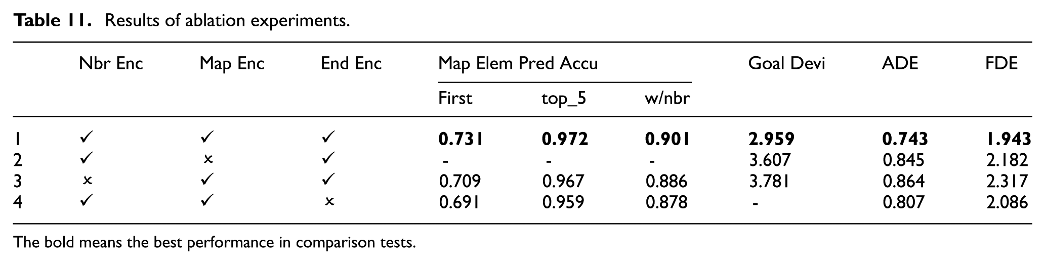
The bold means the best performance in comparison tests.

GoPred progressively narrows down the search space. The TA’s moving intention can be explicitly illustrated by the most likely map element that the TA will reach and the estimated goal point. Accurate estimation of these two parts relies on specific constraints in the training process. In Table 12, the results of map element matching accuracy and goal deviation from the estimation to the ground truth, as well as ADE and FDE, are shown when different combinations of loss functions are used in the model training.

Table 12.

Results while different loss functions are used.

	Goal loss	Map matching loss	MSE	Map Elem Pred Accu			Goal Devi	ADE	FDE
				First	top_5	w/nbr
1	✓	✓	✓	0.731	0.972	0.901	2.959	0.743	1.943
2	✗	✓	✓	0.728	0.972	0.899	21.133	0.764	2.006
3	✓	✗	✓	0.073	0.334	0.182	3.185	0.795	2.068
4	✗	✗	✓	0.005	0.123	0.050	21.130	0.796	2.099

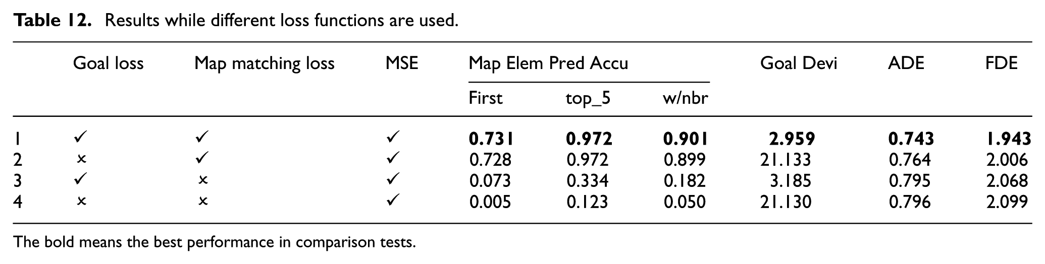
The bold means the best performance in comparison tests.

In Test 3, it is obvious that excluding the map element matching loss leads to a remarkable increase in map element estimation error, the matching accuracy of which is as low as 7.3%. The ADE and FDE increase by 2.8% and 6.4%, respectively. Though the goal estimator still functions, it uses encodings of less relevant map elements, thereby degrading the performance. In Test 2, the goal point estimation loss is omitted. The model still focuses on proper map elements within the AOI. However, without the goal estimation loss, the encodings of map elements and neighbour interactions are not fused optimally, leading to a decrease in the prediction accuracy compared to the model that employs all three loss components. In Test 4, only MSE loss is used during training. Though the model still achieves acceptable prediction accuracy by learning from dynamic scene context, the performance degrades and the interpretability declines because the motion intention is not clear, with first rank hit rate being as low as 0.5% and the goal deviation being as large as 21.13 m.

Conclusions

The research presents a goal-oriented trajectory prediction framework for urban intersections, characterised by low latency and lightweight architecture. Leveraging fragmented map elements, the model enhances prediction accuracy and interpretability by progressively narrowing the inference space and focusing on the most influential map elements. Experimental results have shown that:

• (1) By incorporating behavioural constraints, the proposed cBFS can uniformly explore AOI in both longitudinal and lateral directions and reflect real-world driving dynamics. It can provide robust performance across diverse road scenarios, handle topological variations, achieve minimal missing rates and maintain computational efficiency.

• (2) The prediction model accurately identifies map elements that the TA is likely to reach, enhancing prediction accuracy.

Prediction interpretability is improved by estimating agents’ intentions through the most relevant map elements and grounding corresponding goal points based on this information. This approach provides valuable insights into the model’s understanding of movement intentions and subsequent destinations.

The flexibility of cBFS in setting search limitations along both longitudinal and lateral lanes allows adaptation to diverse application scenarios. The proposed goal-oriented prediction model can fuse both RL and SA information, making it suitable for various scenes and agent classes.

To further validate the framework’s generalisation ability, future work will augment it by incorporating additional scenarios through data merging with datasets such as highD and Argoverse. This will introduce variability in scenarios, enabling further exploration of adaptive capabilities.

Additionally, the proposed prediction model can be extended to better account for prediction uncertainties. Accurate trajectory predictions facilitate risk assessment and trajectory planning, while uncertainty-aware predictions better accommodate ambiguous intentions and perceptual noise.

A straightforward refinement of the proposed framework to address uncertainty is training the model to output trajectories with a Gaussian distribution. Additionally, the estimated top K most likely map elements indicate driving intentions and can serve as initial prediction proposals. Multiple trajectories may thus be generated from these probabilistic intermediate outputs, enabling multi-modal prediction. This approach mitigates the risk of uni-modal predictions learning average manoeuvres across diverse driving intentions.

Uncertainty-aware trajectory prediction supports obstacle avoidance in trajectory planning. However, handling the uncertainty is still an open challenge. In multi-modal prediction, the prediction with the highest probability is not guaranteed to have the least prediction errors. Adopting predictions from all modals often results in overly conservative plans due to overreacting to low-probability branches, while relying solely on the most probable modal can lead to collisions due to overconfidence. Consequently, the practical implications of prediction outcomes in planning tasks require further exploration.