
Abstract
Visual perception plays an important role in autonomous driving. One of the primary tasks is object detection and identification. Since the vision sensor is rich in color and texture information, it can quickly and accurately identify various road information. The commonly used technique is based on extracting and calculating various features of the image. The recent development of deep learning-based method has better reliability and processing speed and has a greater advantage in recognizing complex elements. For depth estimation, vision sensor is also used for ranging due to their small size and low cost. Monocular camera uses image data from a single viewpoint as input to estimate object depth. In contrast, stereo vision is based on parallax and matching feature points of different views, and the application of Deep learning also further improves the accuracy. In addition, Simultaneous Location and Mapping (SLAM) can establish a model of the road environment, thus helping the vehicle perceive the surrounding environment and complete the tasks. In this paper, we introduce and compare various methods of object detection and identification, then explain the development of depth estimation and compare various methods based on monocular, stereo, and RGB-D sensors, next review and compare various methods of SLAM, and finally summarize the current problems and present the future development trends of vision technologies.
Introduction
Environmental perception is one of the most important functions of autonomous driving. The performance of autonomous driving technology is directly influenced by the effectiveness of environmental perception, including factors such as accuracy, resilience to variations in lighting and shadow noise, adaptability to various road conditions, and the ability to function in adverse weather situations. The commonly used sensors in autonomous driving include ultrasonic radar, millimeter wave radar, LiDAR, vision sensors, etc. Although global position technology, such as GPS, BeiDou, GLONASS, etc., is relatively mature and capable of all-weather positioning, there are problems such as signal blocking or even loss, low update frequency, and positioning accuracy in environments such as urban buildings and tunnels. Odometer positioning has the advantages of fast update frequency and high short-term accuracy, but the cumulative error over the long term is large. Although LiDAR has high accuracy, there are several disadvantages, such as large size, high cost, and weather-dependent. Tesla and several companies, such as Mobileye, Apollo, and MAXIEYE, use vision sensors for environmental perception. The application of vision sensors in autonomous driving is based on cameras with advanced artificial intelligence algorithms that facilitate object detection and image processing to analyze obstacles and drivable areas, thus ensuring that the vehicle reaches its destination safely. 1 Visual images are extremely informative compared with other sensors, especially color images. They contain not only the distance information of the object but also the color, texture, and depth information, thus enabling simultaneous lane line detection, vehicle detection, pedestrian detection, traffic sign detection through signal detection, etc. Also, there is no interference between cameras on different vehicles. The vision sensor can also achieve simultaneous localization and map building (SLAM). The vision information is obtained from real-time camera images, providing information that does not depend on a priori knowledge and has a strong ability to adapt to the environment.
The main applications of vision-environmental perception in autonomous driving are object detection and identification, depth estimation and SLAM. Vision sensors can be divided into three broad categories according to how the camera works: monocular, stereo, and RGB-D. The monocular camera has only one camera, and the stereo camera has multiple cameras. RGB-D is more complex and carries several different cameras that can read the distance of each pixel from the camera, in addition to being able to capture color images. Moreover, the integration of vision sensors with machine learning, deep learning, and other artificial intelligence can achieve better detection results. 2 In this paper, we will discuss the following three aspects.
(1) Vision-based object detection and identification, including traditional methods and methods based on deep learning;
(2) Depth estimation based on monocular, Stereo, RGB-D and the application of deep learning;
(3) Monocular SLAM, Stereo SLAM, and RGB-D SLAM.
Object detection and identification
Traditional object detection and identification methods
In autonomous driving, identifying road elements such as roads, vehicles, and pedestrians and then making different decisions are the foundation for the safe driving of vehicles. The workflow of object detection and identification is shown in Figure 1. The image acquisition is made by cameras that take pictures of the surrounding environment around the vehicle body. Tesla 3 uses a combination of wide-angle, medium-focal length, and telephoto cameras. The wide-angle camera has a viewing angle of about 150° and is responsible for recognizing a large range of objects in the near area. The medium focal length camera has a view angle of about 50° and is responsible for recognizing lane lines, vehicles, pedestrians, traffic lights, and other information. The view angle of the long-focus camera is only about 35°, but the recognition distance can reach 200–250 m. It is used to recognize distant pedestrians, vehicles, road signs, and other information and collect road information more comprehensively through the combination of multiple cameras.
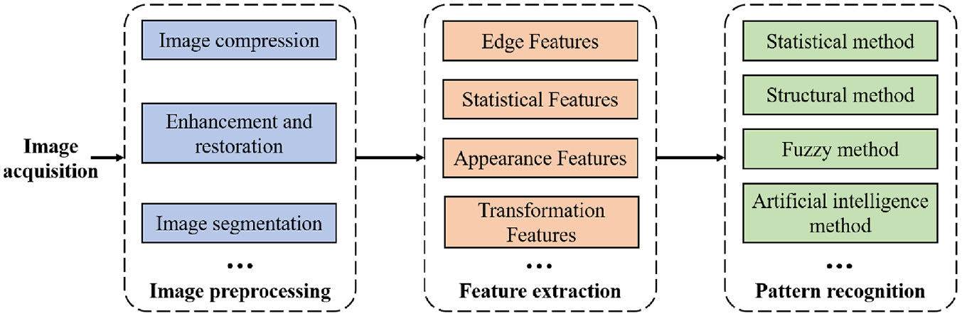
Object detection and identification process, including image acquisition, image preprocessing, image feature extraction, image pattern recognition, etc.
Image preprocessing eliminates irrelevant information from images, keeps useful information, enhances the detectability of relevant information, and simplifies data, thus improving the reliability of feature extraction, image segmentation, matching, and recognition. This process mainly includes image compression, image enhancement and recovery, image segmentation, etc.
(1) Image compression can reduce the processing time and the memory size required. Currently, image compression methods include discrete Fourier transform compression, 4 discrete cosine transform compression, 5 NTT (Number Theory Transformation) compression, 6 neural network compression, 7 wavelet transform compression, 8 and so on. Among them, wavelet transform is more widely used because of its high compression ratio, fast compression speed, and strong anti-interference capability. Furthermore, the grayscale image can compress the color image consisting of Red, Green and Blue channels acquired by the vision sensor into a grayscale map that is represented by grayscale values only. In this way, the distribution and characteristics of color and brightness of the image can be fully reflected, and the processing time is reduced. The common methods for grayscale images include the fractional method, the maximum method, and the average method.
(2) Image enhancement and recovery are used to improve image quality, remove noise, and improve image clarity. Image enhancement techniques are mainly divided into the spatial domain method and the frequency domain method. The spatial domain method9–11 is mainly used to directly compute pixel grayscale values in the null domain, such as image grayscale transform, histogram correction, image null domain smoothing and sharpening, pseudo-color processing, etc. The frequency domain method is used to compute transformation values in some transformation domains of the image, such as the Fourier transformation. 12
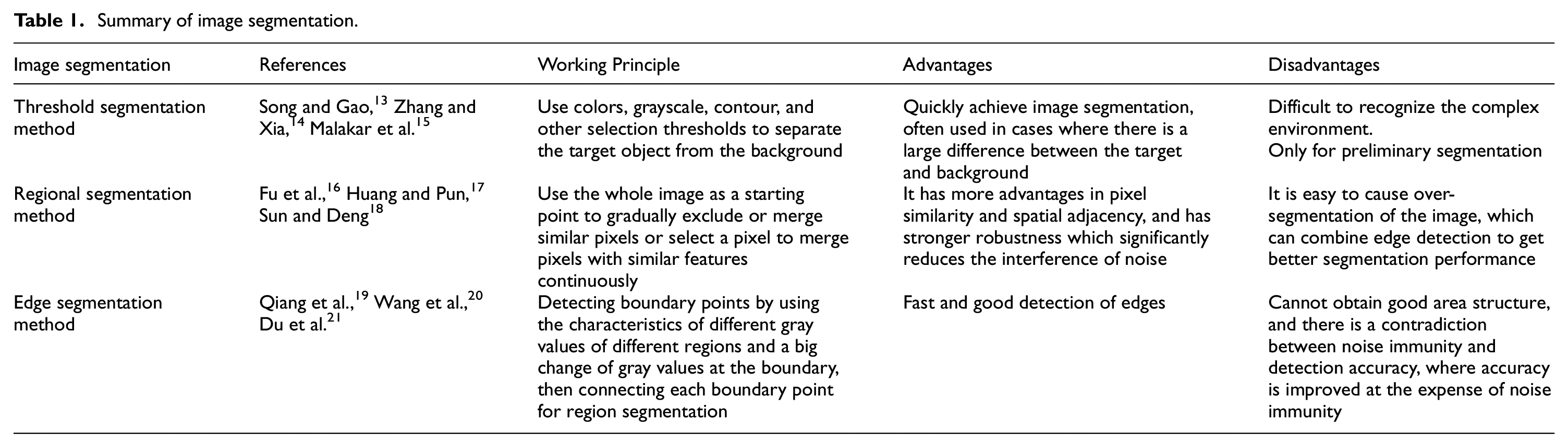
(3) Image segmentation divides an image into several specific regions with unique properties and then extracts the target. This method is a prerequisite for image recognition, and its performance directly affects the quality of image recognition. The main image segmentation methods are threshold segmentation, region segmentation, edge segmentation, and specific theoretical segmentation methods such as mathematical morphology-based, neural network-based, genetic algorithm based, etc. Several major image segmentations are summarized in Table 1 and their segmentation results are shown in Figure 2.
Summary of image segmentation.
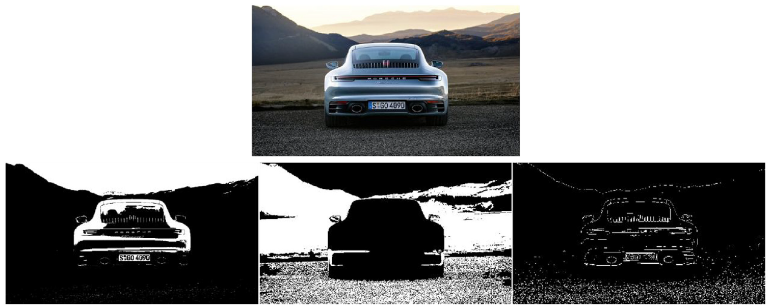
The top is the original image, and the bottom is the image after threshold, region, and edge segmentation, respectively.
The difficulties of image preprocessing include the road information in images with poor quality, which will further deteriorate after grayscale conversion. For example, characters in license plates are easily distorted or lost in preprocessing, and most of the current methods are still lossy compression, therefore, better compression and enhancement of image processing are necessary. Dubé 22 proposed compression by substring enumeration (CSE) to process images by preserving the binary data field for the degradation of performance during grayscale conversion of color images. Qi et al. 23 proposed a JPEG-LS compression algorithm with high compression reliability and low complexity and easy hardware implementation. Sugimoto and Imaizumi 24 proposed a lossless enhancement method that guarantees reversibility while enhancing brightness contrast saturation, and the enhancement level was variable to adjust the visual effect flexibly. In addition, due to illumination, road information is likely to be excessively gray or bright, and binarization processing under such conditions should be discussed on a case-by-case basis, corresponding to special segmentation thresholds. Moreover, due to the complex background and rich edge information in the image, it will not only increase the difficulty of identification, but also cause misjudgment of the system. So the method of handling this information is also one of the difficulties.
It is necessary to extract the required features and calculate the feature values based on image segmentation in order to complete the identification of objects in images. The key to vehicle identification lies in quickly extracting features and achieving accurate matching. The main features are shown below.
(1) Edge Features
The detection operators for edge features include Canny operator, 25 Prewitt operator, 26 Sobel operator, 27 Laplacian operator, 28 etc. The Canny operator has good resistance to noises and uses two different thresholds to detect strong and weak edges, respectively, which performs even better for detecting objects with blurred boundaries. The Roberts operator is better for images with steep low noise, but the extracted edges are coarse, so the edge positioning is not very accurate. The Sobel and Prewitt operators are better for images with noise and gradual changes in grayscale value and are more accurate for edge positioning. The Laplacian operator locates the step edge points in the image accurately but is very sensitive to noise and easily loses orientation information resulting in discontinuous detected edges.
(2) Appearance Features
Appearance features mainly include edges, contours, texture, dispersion, and topological characteristics of the image. Chopra and Alexeev 29 obtained the Gray-level co-occurrence matrix (GLCM) by computing the grayscale image and then calculated the partial eigenvalues of the matrix to represent the texture features of the image. Li, 30 Wang and Liu 31 completed the terrain classification by combining the geometric classifier and color classifier. Real-time ground information can be obtained with continuously updating the 3D data of the terrain surface collected by the vehicle driving.
(3) Statistical Features
Statistical features mainly include histogram features, statistical features (such as mean, variance, energy, entropy, etc.), and statistical features describing pixel correlation (such as autocorrelation coefficient and covariance). Seo et al. 32 performed stereo matching by extracting the vehicle taillight center point from the left camera and right camera, and detected the vehicle ahead using directional gradient histogram features.
(4) Transformation Coefficient Features
It includes the Fourier transformation, Hough transformation, Wavelet transformation, Gabor transformation, Hadamard transformation, K-L transformation, etc. Niu et al. 33 used an improved Hough transformation to extract small line segments of the lane. It identifies lanes by clustering small line segments using a density-based clustering algorithm with noise and by curve fitting. The experimental results show that the detection is better than the linear algorithm and is robust to noise.
(5) Other Features
Images include pixel grayscale values, RGB, HSI, and spectral values. Researchers in Sravan et al. 34 proposed a vehicle detection method based on color intensity separation, which uses intensity information to filter the Region of Interest (ROI) of light changes, shadows, and clutter background, and then detects vehicles based on the color intensity difference between vehicles and their surroundings. Anandhalli and Baligar 35 converted RGB video frames captured by RGB-D to color gamut images, whose noise can be reduced or eliminated for each frame. This method distinguishes the color characteristics of vehicles more accurately and achieves tracking of vehicles.
The difficulty of image feature extraction is that in practical situations objects may blend into the background and be difficult to be recognized due to background interference, or only a part of the object is visible due to occlusion. To solve this, Kurbatova and Pavlovskaya 36 proposed a method for detecting partially occluded road information by first performing contour segmentation based on the HSV color space, then calculating element values for each line segment and comparing them with a threshold value, and removing shadows with a gamma correction method. Enze and Miura 37 proposed a method to separate the target and noise by detecting the moving target from the difference of continuous images by the difference obtained by subtraction of the current frame and the previous frame, then automatically calculating the threshold value by Otsu’s Threshold Method, and finally by brightness histogram and digitized images for noise removal. Huang et al. 38 proposed an interference removal method combining feature extraction and function fitting, which is achieved by extracting the statistics and spatial location of the stripe noise, and then coarse and fine-processing the image in two steps.
Pattern recognition is performed based on the extracted features, which compares the object of interest with existing known patterns to determine its category. Pattern recognition methods can be divided into different categories based on the features used, for example, shape features, color features, texture features, etc. Based on the recognition methods used, it can be divided into statistical pattern recognition, 39 structural pattern recognition, 40 fuzzy pattern recognition, 41 neural network pattern recognition, 42 etc. Among them, the principle of statistical pattern recognition is to use a given finite number of sample sets to divide the d-dimensional feature space into c regions, each region corresponding to each class, by learning algorithms under the condition of known statistical model of the research object or known discriminant function class according to certain criteria. The main methods include the discriminant function method, k-nearest neighbor classification method, nonlinear mapping method, etc. Fuzzy pattern recognition is a method to represent a specific category or object to be identified by a fuzzy set. It greatly improves the pattern recognition capability based on fuzzy mathematics and is one of the most promising fields of application. However, pattern recognition currently suffers from undetected or incorrect detection due to the lack of effectively extracted feature points as well as the original object’s perspective change, deformation, and shape difference between individuals.
The current difficulties in pattern recognition include the selection and formal representation of features and the difficulty of establishing classification rules. In recent years, advances in classifiers have greatly improved the classification performance, but the computation of these methods is still complex and there are still difficulties in classifying large sample sets. In addition, the development of deep learning has given a new direction to pattern recognition by constantly adapting to new samples without losing the classification performance of the original trained samples, which makes the neural network-based methods gradually outperform other methods in terms of performance.
In general, the development of traditional object identification is mainly based on different features to optimize detection methods. Among them, Haar is widely used due to its fast extraction speed, its ability to express information about multiple edge changes of the object, and its fast computation using integral maps. The detection process requires framing the position as well as the size of the object in the image. In order to find the candidate frame, it is necessary to traverse the image from left to right and from top to bottom. The multi-scale search is performed by scaling a set of image sizes to obtain an image pyramid. This sliding window based region selection strategy is not targeted, so traditional object identification methods generally suffer from window redundancy and because of their weak features, a detector needs to be trained for each class, which is time consuming and has a large overall computational effort. Hand-designed features are also not very robust to changes in diversity and are more limited in their ability to express shallow-level features. In addition, it may cause information loss when solving each sliding window. However, by removing the areas that are not the desired objects through Selective Search or EdgeBox based on color clustering and edge clustering, the detection accuracy can be improved to some extent and the identification time can be reduced. It should be noted that traditional detection methods tend to saturate the detection performance as the amount of data increases, unlike deep learning methods, which get better and better when more and more data are distributed to match the actual scene. However, one advantage of the traditional approach is that the hierarchy is simple and thus easy to debug, which is suitable for cases with fewer data.
Due to the complexity of the road environment, vehicles must rely not only on a single forward-facing camera but also on the surrounding view. Blind spots have led to many car accidents, so detecting pedestrians and vehicles in blind spots is critical. Surround-view cameras or panoramic video monitoring (AVM) systems, as shown in Figure 3, stitch together images from all directions of the car and identify road signs, curbs, and nearby vehicles, making it easy for drivers to look around, thereby reducing the number of car accidents. In addition, BEV (Bird’s Eye View) can better conduct 3D detection so as to realize automatic driving. 43
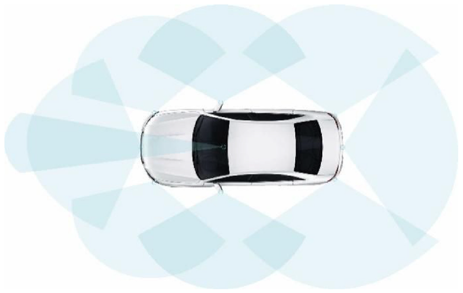
Surround-view cameras.
Fujitsu’s Wrap Around View 44 provides a real-time updated view on the basis of splicing the panoramic view together. The driver can select the best view for different situations, including the “third-party” view and images of the vehicle itself and its surroundings. Su et al. 45 further developed 3D AVM based on 2D AMV, which can expand the visual coverage, thus helping the driver to determine the collision distance with another vehicle on narrow roads and improving driving safety. Tesla’s vision system adopts three cameras in the front of the car, one in the rear, and two in the side rear and side front, respectively, to achieve a total of eight cameras for accurate blind zone monitoring and target-ranging functions. In general, these solutions can be divided into 2D surround-view camera systems and 3D surround-view camera systems. The former provides a traditional flat bird’s eye view of the vehicle’s surroundings on the cockpit display. The latter displays the vehicle and its surroundings in a spherical 3D representation so that the desired view can be obtained from any angle around the vehicle. Therefore, this method is more effective for perimeter surveillance.
The main techniques used in Surround View Cameras include image correction, top view transformation, image matching, image fusion, etc. The images captured by the Fisheye Lens are distorted and therefore require calibration and correction. The most commonly used calibration method for Surround View Cameras is the Zhang Zhengyou calibration method, 46 which yields stable results and is easy to use. The direct linear transformation method 47 uses the one-to-one correspondence between multiple 3D point coordinates and pixel coordinates to compute a linear system of equations to obtain the camera model. However, this method does not consider the nonlinear distortion of the camera lens, so the accuracy is not high. Therefore, Tang et al. 48 proposed an improved Tsai calibration method. This method first solves the linear relationship between pixel coordinates using the direct linear transformation method, and then takes this linear relationship as the initial value, combined with the lateral and radial distortion of the lens. It uses an optimization algorithm to optimize the internal and external parameters of the camera, which solves the low accuracy problem of the direct linear transformation method. However, Tsai method cannot calibrate all the external parameters through one plane, which is unstable for nonlinear operation results, so Scaramuzza et al. proposed an omni directional calibration method. 49 It uses a polynomial to approximate the way to solve the internal and external parameters of this lens based on the information of the corner points of the calibration module and the mathematical model by the conversion relationship between the world coordinate system, the fisheye lens coordinate system and the planar imaging coordinate system. The frequently used fisheye correction algorithms can be divided into projection model-based correction methods and 2D and 3D space-based correction methods. Since the final rendering of the panoramic monitoring is a top view, the corrected map must first be transformed into a top view, mainly based on camera parameters and based on the projection matrix. Philion and Fidler 50 proposed a Lift, Splat, Shoot three-step approach, which first generates 3D features from 2D image features (Lift), then transforms the 3D features into a BEV feature map (Splat), and finally performs relevant task operations on the BEV feature map (Shoot). In addition, they compared the importance of each view. Li et al. 51 further proposed BEVDepth, which adds depth information to the top view. In 2020, Carion et al. 52 proposed DETR3D, which feeds multi-scale features into 2D to 3D Feature Transformation to perform panoramic segmentation. Although DETR3D merges multiple features from two adjacent views in the overlapping region, it still suffers from insufficient feature aggregation. 53 Therefore, in 2022 Liu et al. 54 transformed the circumferential features into 3D domains by encoding the 3D coordinates from the camera transformation matrix. The detection effect is greatly improved.
The image stitching methods include SIFT-based stitching methods 55 and SURF-based stitching methods 56 which are improved based on SIFT. The SIFT (Scale Invariant Feature Transform) method first finds the extreme points, delete the points with small influence, and then uses the Hessian matrix to delete the edge points to calculate the description information of the feature points. Then, the feature points in each image are compared, and the points with similar features are considered as the same position for stitching. In Liu, 57 the quality of the panoramic view is enhanced by using six Fisheye Lens, improving the SIFT algorithm for image matching, and improving the fading-in and fading-out algorithm for better image fusion. The SURF (Speeded Up Robust Features) method uses Haar wavelet response and image integration when calculating the descriptive information of feature points, thus collecting feature information quickly and improving the accuracy of feature point matching simultaneously.
Deep learning-based object detection and identification
Compared with traditional object detection and identification, deep learning requires training based on a large dataset but brings better performance. Traditional object identification methods do feature extraction and classifier design separately and then combine them together. In contrast, deep learning has more powerful feature learning and feature representation capabilities by learning the database and mapping relationships to process the information captured by the camera into a vector space for recognition through neural networks. The object detection and identification model is shown in Figure 4. The “Backbone” in the figure refers to the convolutional neural network for feature extraction that has been pre-trained on a large dataset and has pre-trained parameters. The “Neck” represents some network layers used to collect feature maps in different stages. The “Head” represents the type and location of bounding boxes.
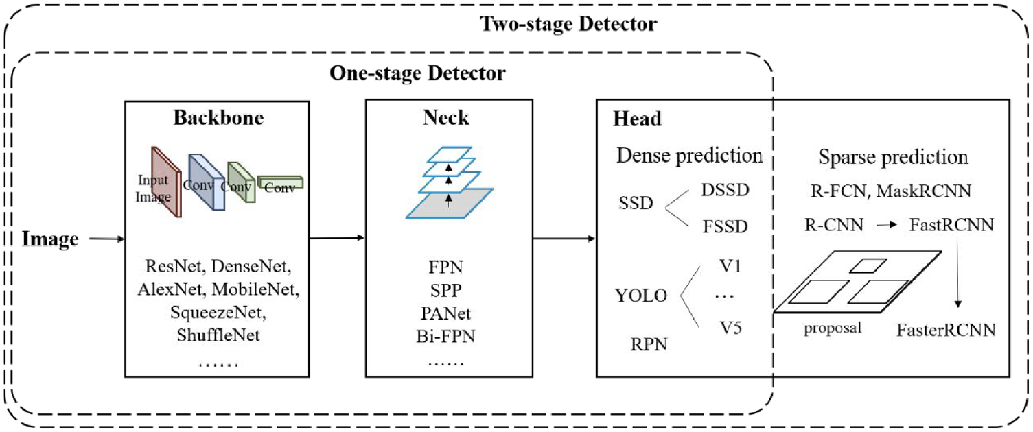
Object detection and identification module, mainly including Backbone, Neck, and Head.
For the “Backbone,” AlexNet 58 was the first application of deep learning technology to large-scale image classification. Compared to other deep learning networks, AlexNet used five layers of convolutional layers and three layers of fully connected layers, the activation function replaced sigmoid with ReLU, and Dropout is used in the first two layers, that is, randomly deactivating some cells to reduce the overfitting problem. The object identification error rate reaches 17%. However, most of the previous CNN-based methods suffer from the large storage space required, computational inefficiency, and the size of the perceptual region is limited by the pixel block size. Therefore, in 2014, Long et al. 59 proposed a full convolutional neural network (FCN) to implement pixel-level segmentation using a deep convolutional neural network approach. It can accept input images of arbitrary size and avoids the problems of double computation and space wastage due to the use of neighborhoods. In response to the long-standing lack of knowledge about the intrinsic mechanisms of these models, Zeiler and Fergus 60 proposed a ZFNet to visualize the features learned by a CNN through deconvolution for object identification, while adjusting the size and step size of the AlexNet filter to achieve an error rate of 11.7%. In 2015, Szegedy et al. 61 proposed GoogLeNet using a Network in the network (NiN) based network, the Inception module is shown in Figure 5. By extracting information in parallel through convolutional and max-pooling layers of different sizes, the 1 × 1 convolutional layer can significantly reduce the number of parameters, decrease the model complexity, and reduce the identification error rate to 6.7%.
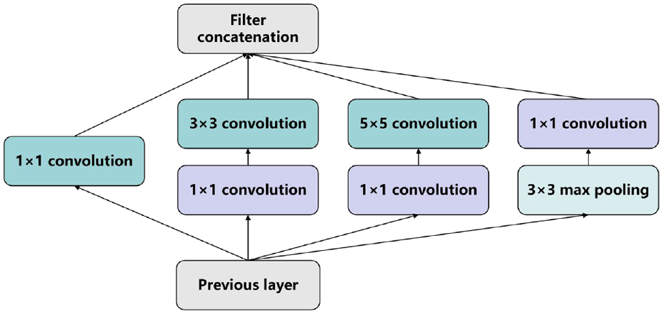
Inception module.
In 2016, Saini and Rawat 62 proposed ResNet to solve the gradient vanishing problem during backpropagation. It improves the efficiency of information propagation by adding directly connected edges to the nonlinear convolutional layers to reduce the error rate to 3.6% and increases the network depth to hundreds of layers, so it can train deep networks without adding a classification network in the middle to provide additional gradients like GoogLeNet. For the problem that the same target may be misjudged as different targets due to the use of only local signals in the prediction of large targets and that small targets may be ignored, Noh et al. 63 proposed DeconvNet. This method adopted an inverse process opposite to the forward pass process and introduced deconvolution and anti-pooling layers to reduce the feature map to the original size and achieve the segmentation after the mirroring process. Google 64 proposed Deeplab V2 with an ASPP structure based on Deeplab V1, which can pool the original feature maps at different scales and then fuse the results of each scale to achieve better identification results. However, in traditional convolutional neural networks, when information about the input or gradient passes through many layers, it may disappear when it reaches the end of the network. In 2017, DenseNet 65 developed based on ResNet, introduced a direct connection between any two layers with the same elemental graph size, such that L connections were increased to L(L + 1)/2 connections, as shown in Figure 6, where H(i) includes Batch Normalization (BN), ReLU, Pooling, and Convolution (Conv). The traditional feedforward architecture can be considered as an algorithm with a state that is passed layer by layer and therefore does not need to relearn redundant feature maps. One of the major advantages of DenseNet is that it improves the flow of information and gradients throughout the network, making it easier to train. Each layer can access the gradients directly from the loss function and the original input signal, which both drastically reduces the number of parameters in the network and alleviates the problem of gradient vanishing to some extent, and enhances the transmission of features of its structure. And in the same year, Xie et al. 66 proposed ResNeXt, which continues ResNet and Inception and adds residual connectivity. Chen et al. 67 proposed Deeplab V3, which optimized DeeplabV2. The Atrous Spatial Pyramid pooling (ASPP) structure in Chen et al. 64 introduced tandem multi-scale null convolution and used the Batch Normalization method to improve the segmentation accuracy, thus allowing better object identification.
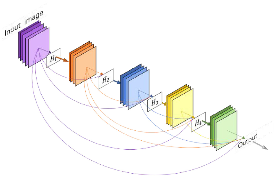
A 5-layer DenseNet.
Although the performance of these network models has been greatly improved, the scale and speed of operation are not suitable for practical applications such as autonomous driving. Therefore, MobileNet proposed in Howard et al. 68 reduces the computational cost to 1/8–1/9 by replacing the standard convolution with a depth-separable convolution and splitting the standard convolution into one depth convolution and one point-by-point convolution. ShuffleNet proposed in Zhang et al. 69 uses grouped convolution to reduce the number of training parameters. Ma et al. 70 improved ShuffleNet by dividing the input feature map into two branches and finally connecting branches and merging them with Channel Shuffle, which resulted in better identification. In 2020, Wang et al. 71 by inserting an ELU function as an activation function based on MobileNet, the disappearance of the gradient in the linear part can be alleviated, and the nonlinear part is more robust to noise caused by input changes. Although many network structures are reducing the computational effort by various methods, similar feature maps still exist, and on the other hand, these similar feature maps are also valuable to be utilized. For this problem Han et al. 72 proposed GhostNet, which first performed a convolutional operation on the input feature map and then performed a series of simple linear operations to generate the feature map. Thus, it reduces the number of parameters and computations while achieving the performance of traditional convolutional layers. However, deep convolutional networks suffer from the loss of output spatial resolution due to the pooling layer. The mixed extraction of many different features results in less accurate information processing, such as boundaries. Takikawa et al. 73 proposed a dual-stream (shape stream and classical stream) CNN that processes information in parallel and Gated Convolutional Layer (GCL) that allows classical streams and shape streams to interact in the middle layer for better identification. On the other hand, most lightweight networks have a relatively simple body structure, which leads to low system performance. In response to this, in 2021 LDSNet 74 proposed LDSNet, which introduced a feature selection module (FSM). This enables to improve the accuracy of the system image recognition while maintaining the lightweight. To meet the requirements of high accuracy, high real-time and low number of parameters for lane detection algorithms in industrial practice, Wang and Li 75 used UNet as the main structure of the network and applied MoblieNet to the network coding process to ensure the accurate extraction of lane information. To enable real-time vehicle target detection for smartphones in 2022 Sun et al. 76 proposed NanoDet. It removes most of the convolutional layers and uses depth-separable convolution to further improve the computational speed of the detector. Two-stage detectors are always not efficient due to their multi-stage nature, while one-stage detectors have a balance of speed and accuracy but are difficult to apply in practice due to their large size. Therefore, in 2022 Shi et al. 77 proposed DPNET. Their backbone includes a stem and a set of ASBs (Attention-based Shuffle Block), resulting in parallel structure of low-resolution path and high- resolution path, while combining a self-attentive mechanism to improve the target detection of dual-path structure. In Kang et al., 78 Domain-specific Lightweight Network (DLNet) was proposed to reduce the number of parameters and running time for object detection by training objects with higher frequency for better application in feature intelligence applications.
For “Head,” there are usually two groups of object detection algorithms, namely two-stage object detection algorithm and one-stage object detection algorithm. The former group of algorithms first generates a series of candidate frames as samples and then classifies the samples using a convolutional neural network, which has better detection accuracy and localization precision. The latter group of algorithms does not generate candidate frames. Instead, it directly transforms the target frame localization problem into a regression problem, and the algorithm is faster. The two-stage object detection algorithms include mainly RCNN series. RCNN is first proposed in Long et al., 59 which first uses Selective Search to search for regions where objects may be present, then inputs these regions into AlexNet with the same size to obtain feature vectors, and finally uses SVM for classification to obtain detection results. However, RCNN has the problem of extracting features for the same region several times, so He et al. 79 proposes SPP-Net. In the feature extraction stage, it directly extracts features for a whole image to get the feature map, which avoids repeated extraction and thus improves the operation speed of the algorithm. Then, region proposals are found in the feature map, and the fixed feature vectors are extracted by spatial pyramid pooling, which greatly improves the operation speed. The Fast R-CNN proposed by Girshick and Fast 80 introduces an ROI pooling layer, the feature map output by Selective Search is ROI Pooling to get the feature vector, and softmax is used instead of SVM to classify the class of ROI compared to SPPNet. Ren et al. 81 proposed Faster R-CNN using Region Proposal Networks instead of Selective search. It goes through the feature map (from the convolutional layer) with a set of windows of different aspect ratios and sizes and uses these windows as candidate regions for classification and object localization. The object recognition speed and accuracy are greatly improved. However, the faster R-CNN is not shared after ROI pooling, so Dai et al. 82 used the full convolutional network to create shared convolution of the layers after ROI and convolve only one feature map, and the detection efficiency is further improved.
One-stage object detection algorithms include YOLO and SSD. YOLO (You Only Look Once), which treats object detection as a regression problem and uses the entire image as input to train the model. Therefore, it can detect the information of the whole picture rather than the partial picture information detected by the sliding window. Although this approach decreases accuracy, but can greatly improve the detection speed. In 2015, Redmon et al. 83 proposed YOLOv1, as shown in Figure 7. It first splits the input image into a grid of cells and then marks the position of the object with a boundary box. If the center of the bounding box falls within a cell, this cell is responsible for predicting this object. However, when there are multiple objects whose centers fall in a single cell, the object may not be detected, or the accuracy of the detection is reduced. To solve this problem, Redmon and Farhadi 84 proposed YOLOv2, which removed the final fully connected layer from YOLOv1 and used convolution and anchor boxes to predict the bounding boxes. The identification rate and speed were improved. Redmon and Farhadi 85 proposed YOLOv3 to further improve the model by improving the single-label classification of YOLOv2 to multi-label classification and removing the pooling layer, using all convolutional layers for downsampling, and improving the network’s ability to characterize the data by deepening the network and the use of FPNs. However, there are still difficulties in running in real-time. So Bochkovskiy et al. 86 proposed YOLOv4 that split the channel into two parts, with one part performing the computation of convolution and then concatting the other part together, thus reducing the computation and being able to guarantee accuracy. YOLOv5 proposed in Zhu et al. 87 is more flexible and has four network models, but the performance is not as good as YOLOv4.
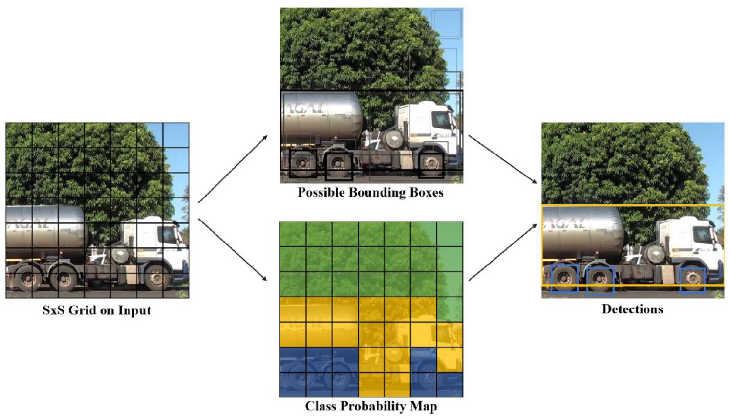
YOLO schematic 88 identifies the objects falling in each cell by dividing the image into a network of cells.
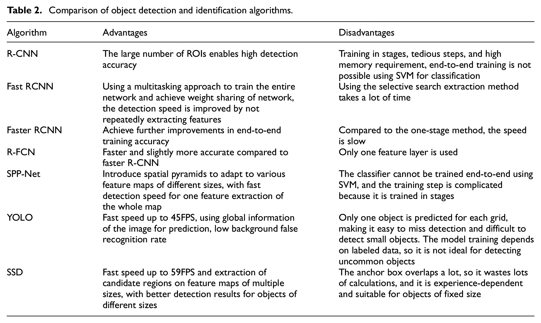
SSD (Single Shot MultiBox Detector) was proposed by Liu et al. 89 Unlike Yolo which does detection after a fully connected layer, SSD uses CNN to perform detection directly and employs a multi-scale feature map. Large-scale feature maps (near-input feature maps) can be used to detect small objects, while small-scale feature maps (near-output feature maps) are used to detect large objects, which makes SSD better than Yolo in terms of accuracy. Lin et al. 90 argues that there are only a few objects in many detection areas of the picture, which leads to unbalanced training sample categories and the poor performance of a one-stage object, so they propose RetinaNet based on Cross Entropy loss. When the classification error is low, a lower weight is given. The detection performance is improved by giving higher weights for the loss when the classification error is higher. Comparison of several algorithms is shown in Table 2.
Comparison of object detection and identification algorithms.
Take Tesla as an example, the main input of the system is from cameras at eight different locations. Due to the different camera locations and poses, the image of each camera is first projected onto a virtual camera at a fixed location and pose. ResNet was then used for multi-object identification and preliminary feature extraction, and Tesla used a bi-directional feature pyramid (BiFPN), 91 which combines interlayer feature fusion with multi-resolution prediction and enables easy and fast multi-scale feature fusion. Tesla uses the Transformer self-attention mechanism to combine the camera location information and cross-learning of the features seen by each camera to integrate the images from eight cameras into a complete 360-degree, highly compressed and abstracted information. After that, introduce the timeline from the continuous video and use LSTM, which is a recurrent neural network to obtain various environmental information for auto driving.
For autonomous driving tasks, such as the detection of roads and signal light recognition, Tesla uses HydraNet 92 which has different network components for subtasks, as in Figure 8, where there is a commonly shared backbone, which splits into branches in the head. The use of feature sharing reduces repetitive convolutional computations, while the backbone network can be fixed after fine-tuning, and only the parameters of the detection head need to be trained, resulting in a significant improvement in efficiency and the ability to decouple specific tasks from the backbone.
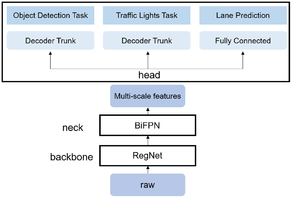
Multi-task learning HydraNets.
Depth estimation
In autonomous driving systems, the proper distance is extremely important to ensure the safe driving of the car, so it requires depth estimation from the images. The goal of depth estimation is to obtain the distance to the object and finally acquire a depth map that provides depth information for a series of tasks such as 3D reconstruction, SLAM, and decision-making. The current mainstream distance measurement methods in the market are monocular, stereo, and RGB-D camera-based.
Traditional monocular depth estimation methods
For fixed monocular cameras and objects, since the depth information cannot be measured directly, therefore, monocular depth estimation is to recognize first and then measure the distance. First, the identification is made by image matching, and then distance estimation is done based on the size of the objects in the database. Since the comparison with the established sample database is required in both the identification and estimation stages, it lacks self-learning function and the perception results are limited by the database, and the unmarked objects are generally ignored, which causes the problem that uncommon objects cannot be recognized. However, for monocular depth estimation applied to autonomous driving the objects are mainly known objects such as vehicles and pedestrians, so the geometric relationship method, 93 data regression modeling method 94 and Inverse Perspective Mapping (IPM) 95 can be used, and SFM(Structure From Motion)-based monocular depth estimation can be achieved by the motion of vehicles. Currently, monocular cameras are gradually becoming the mainstream technology for visual ranging due to their low cost, fast detection speed, and ability to identify specific obstacle types, high algorithm maturity and accurate recognition.
The geometric relationship method uses the pinhole camera imaging principle. It uses light propagation along a straight line to project objects in the three-dimensional world onto a two-dimensional imaging plane, as shown in Figure 9. The vehicle distance can be calculated by the equation in the figure. However, it is required that the optical axis of the camera must be parallel to the horizontal ground, which is difficult to guarantee in practice. Yang et al, 96 Guan et al. 97 improved this by considering the yaw angle of the camera, and the distance measurement is more accurate.
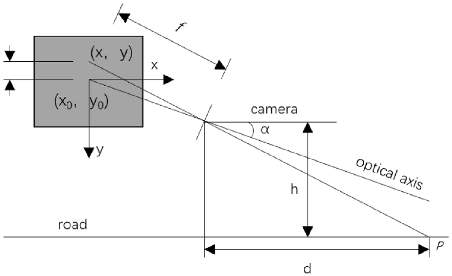
Geometric ranging model, α is the camera pitch angle, h is the camera height, and the projection point of the body p point in the phase plane is (x, y).
The data regression modeling method measures the distance by fitting a function to obtain a nonlinear relationship between the pixel distance and the actual distance. Inverse Perspective Mapping is widely used not only in monocular ranging but also in Around View Cameras. By converting the perspective view into bird’s eye view, as shown in Figure 10. Since BEV has a linear scale relationship with the real road plane, the actual vehicle distance can be calculated based on the pixel distance in the inverse perspective transformed view by calibrating the scale factor, which is simple and easy to implement.
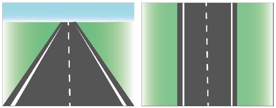
Transformation of the original view of the driveway into BEV through Inverse Perspective Mapping (right).
However, the pitch and yaw motion of the car is not considered, and the presence of pitch angle will make the inverse perspective transformed top view unable to recover the parallelism of the actual road top view, thus producing a large-ranging error. Liu et al. 98 proposed a distance measurement model based on variable parameter inverse perspective transformation, which dynamically compensates for the pitch angle of the camera, with a vehicle ranging error within 5% for different road environments and high robustness in real-time. However, it is impossible to calculate the pitch angle of the camera on unstructured roads without lane lines and clear road boundaries. A pitch angle estimation method without cumulative error is proposed in, Li et al. 99 which uses the Harris corner algorithm and the pyramid Lucas-Kanade method to detect the feature points between adjacent frames of the camera. Its camera rotation matrix and translation vector are solved by feature point matching and pairwise geometric constraints, and parameter optimization is performed using the Gauss-Newton method. Then, the pitch angle rate is decomposed from the rotation matrix, and the pitch angle is calculated from the translation vector.
Structure From Motion (SFM) is to determine the spatial geometric relationship of an object from a 2D image sequence by using mathematical theories such as multi-view geometry optimization to recover the 3D structure by camera movement. SFM is convenient and flexible but encounters scene and motion degradation problems in image sequence acquisition. According to the topology of image addition order in the process, it can be classified as incremental/sequential SFM, global SFM, hybrid SFM, and hierarchical SFM. Besides, there are semantic SFM and deep learning-based SFM. The comparison of different depth estimates and different SFMs is shown in Table 3.
Summary of the main depth estimates and different SFMs.
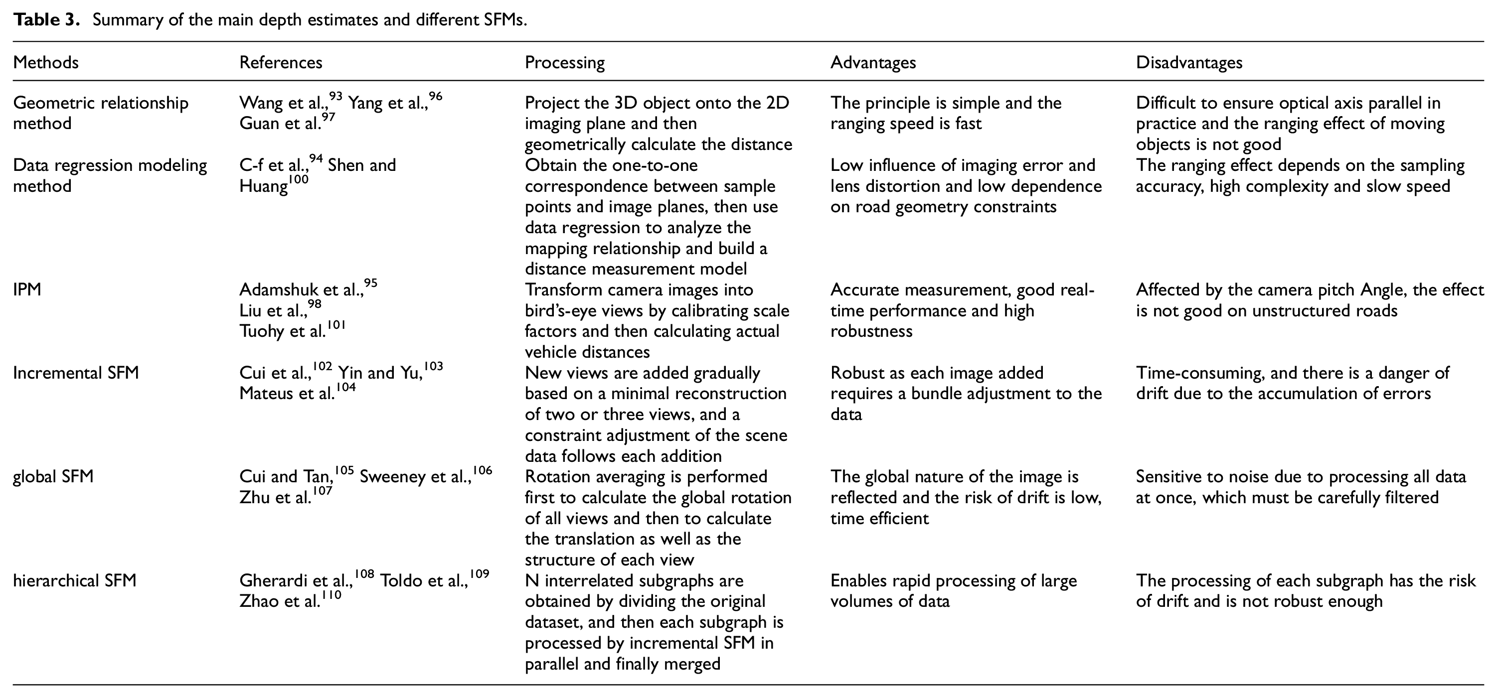
On the other hand, hybrid SFM 111 combines the advantages of incremental SFM and global SFM and is gradually becoming a trend. The pipeline can be summarized as a global estimation of a camera rotation matrix, incremental calculation of the camera center, and community-based rotation averaging method for global sensitive problems. Compared with hybrid SFM, PSFM 112 grouped the cameras into many clusters and was superior in large-scale scenes and high-precision reconstruction. Vijayanarasimhan et al. 113 proposed SFM-Net to estimate the depth and pose of each frame using the photometric consistency principle. Based on this, Zhou et al. 114 proposed SFMLearner with the addition of optical flow, scene flow, and 3D point cloud to estimate depth.
Monocular camera has a high proximity recognition rate, so it is widely used in front collision warning systems (FCWS). But its environmental adaptability is poor, and the camera shakes due to bumps when the vehicle is moving. In Feng, 115 a comparison experiment of three scenarios, stationary, slow-moving, and braking, resulted in taking the arithmetic mean of TTC as the alarm threshold, which can effectively circumvent abnormal situations such as camera shake and thus can be applied to more complex ranges. Bougharriou et al. 116 adopted a combination of vanishing point detection, lane line extraction, and 3D spatial vehicle detection to achieve distance measurement. However, the distance error increases significantly in the case of insufficient illumination and severe obstacle occlusion in front. In Ma et al., 117 it is proposed that the absolute scale and attitude of the system are estimated using monocular Visual Odometry combined with the GPS road surface characteristics and geometrics prior to detecting and ranging the object in front of the vehicle and that the localization of the camera itself and the object can be achieved using the 3D shape change of the object.
Deep learning-based monocular depth estimation
The performance of monocular depth estimation based on deep learning methods has improved significantly in the past few years. Compared with traditional depth estimation methods, its input is the original image captured and the output is a depth map with each pixel value on it corresponding to the scene depth of the input image. Deep learning-based monocular depth estimation algorithms are divided into supervised and unsupervised learning. Supervised learning is able to recover scale information from the structure of individual images and scenes with high accuracy because they train the network directly with ground truth depth values but require datasets such as KITTI, Open Image, Kinetics, JFT-300M, etc. Since depth data is difficult to obtain, a large number of algorithms are currently based on unsupervised models.
Earlier studies used Markov Random Field (MRF) to learn the mapping relationship between input image features and output depth, but the relationship between RGB images and depth needs to be artificially assumed. The model is difficult to simulate the real-world mapping relationship, and therefore the prediction accuracy is limited. In 2014, Eigen et al. 118 proposed to convolve and downsample the image in multiple layers to obtain descriptive features of the whole scene and used them to predict the global depth. Then, the local information of the predicted image is refined by a second branching network, where the global depth will be used as input to the local branch to assist in the prediction of the local depth. In 2015, Eigen and Fergus 119 proposed a unified multi-scale network framework based on the above work. The framework uses a deeper base network, VGG, and uses a third fine-scale network to add detailed information further to improve the resolution for better depth estimation. In 2016, Bao and Wang 120 compared the performance of different convolutional neural network models for vehicle detection, and then adjusted the ZF model for vehicle-specific environments and selected the lower part of the image to compress the detection area to further improve the detection speed and localization accuracy. But it needs to measure at a specific distance and there are limitations in measuring with the vehicle as the reference. In 2018, Fu et al. 121 proposed the DORN framework based on the problem of inherent ordered relations existing between depths. They divided the continuous depth values into discrete intervals and then used fully connected layers to decode and inflated the convolution for feature extraction and distance measurement and the detection effect was significantly improved. In the same year, Wang et al. 122 considered the high accuracy but high cost of LiDAR to convert the input image into point cloud data similar to that generated by LiDAR, and then used an algorithm of point cloud and image fusion to detect and measure the distance to improve the depth information representation. In addition due to the problem of loss of geometric information in the projection process of the image leading to a decrease in the accuracy of detection, Qin et al. 123 proposed MonoGRNet. They obtained the visual features of the object by ROIAlign and then used these features to predict the depth of the 3D center of the object, reducing the uncertainty of the 3D rotation in the perspective transformation. Considering the difficulty of the number of planes and the order of the planes to be regressed in the output feature vector, Liu et al. 124 proposed PlaneNet to implement a segmented reconstruction of the planar depth map from a single RGB image. In 2019, Barabanau et al. 125 improved it by proposing MonoGRNetV2 to extend the centroids to multiple key points and use 3D CAD object models for depth estimation. Kim and Kum 126 proposed BEV-IPM to convert the image from a perspective view to BEV. In the BEV view, the Bottom Box (the contact part between the object and the road surface) is detected based on the YOLO network. Then its distance is accurately estimated using the Box predicted by the neural network. Previous work was more on pixel-level prediction in the discrete domain, Xu et al. 127 proposed a multi-scale feature map using the output of a convolutional neural network based on the depth estimation of two resolutions, and then predicted the depth maps of different resolutions after fusion by continuous MRF. Kundu et al. 128 proposed 3D-RCNN, which first uses PCA to downscale the parameter space and then generates 2D images and depth maps based on each targetlow-dimensional model parameter predicted by the R-CNN. Nevertheless, CNNs can handle global information better only when at lower spatial resolutions. The key to the effectiveness of monocular depth estimation enhancement is that sufficient global analysis should be performed on the output values. Therefore, in 2020 Bhat et al. 129 proposed the AdaBins structure as shown in Figure 11, which combines CNN and transformer. Using the excellent global information processing capability of the transformer, combined with the local feature processing capability of CNN, the accuracy of depth estimation is greatly improved.
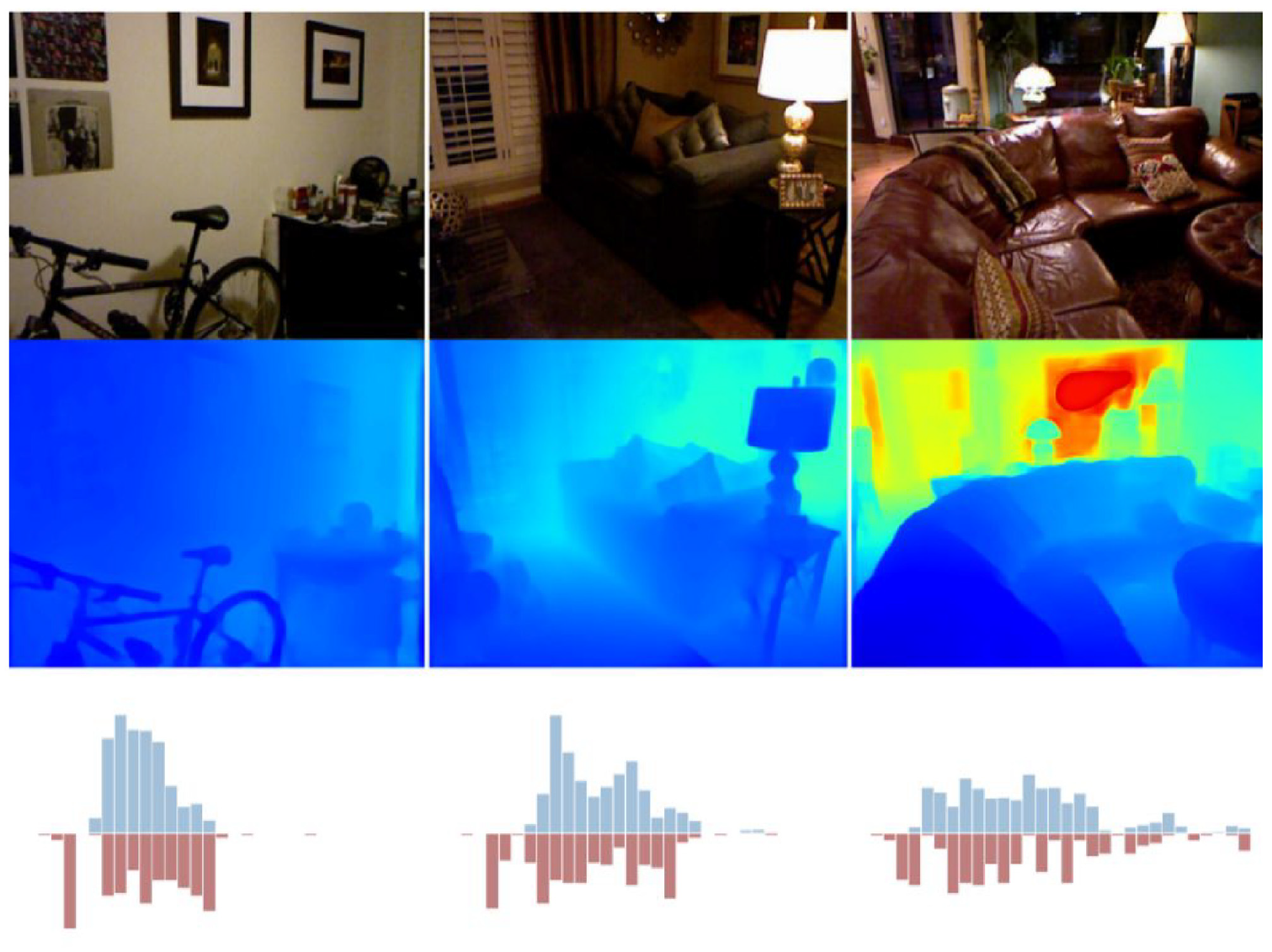
AdaBins 129 top is original. The middle is the depth map, and the bottom is the histogram of depth values of the ground truth and predicted adaptive depth.
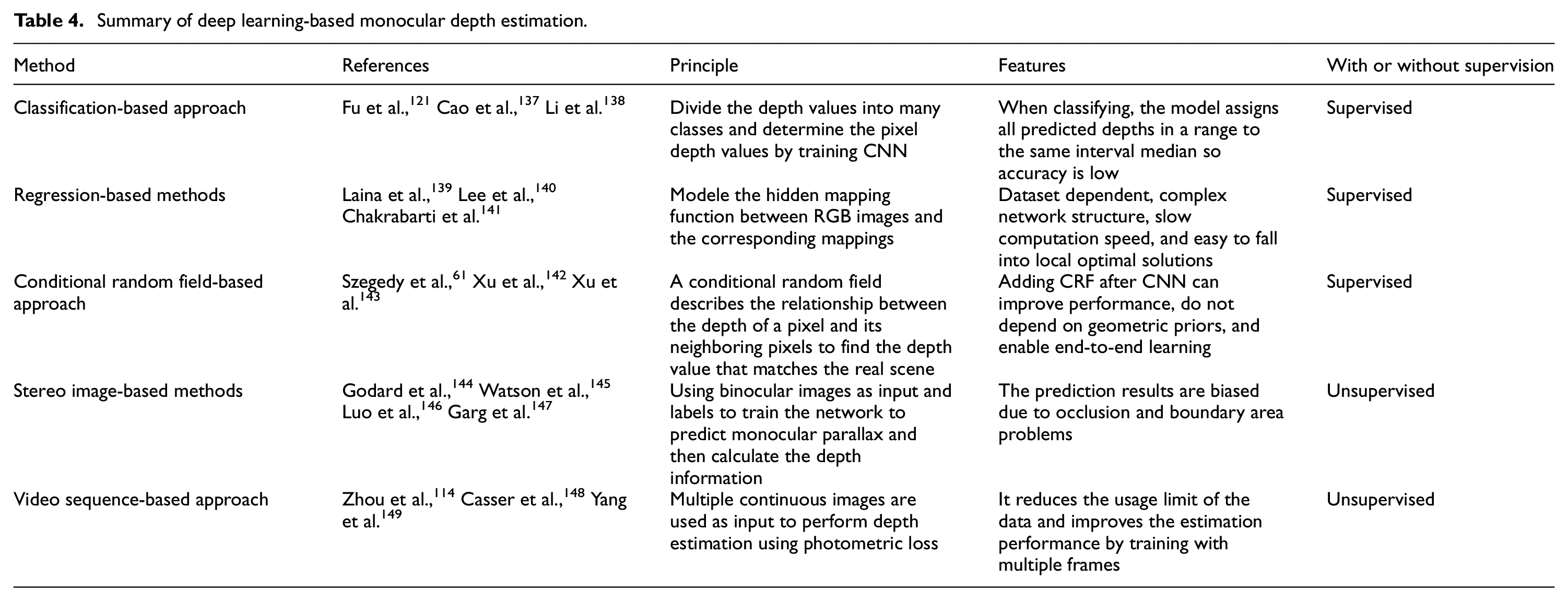
According to, Shen et al. 130 an end-to-end convolutional neural network framework is utilized for vehicle ranging in order to cope with measurement errors due to light variations and viewpoint variations. The algorithm is based on converting RGB information into depth information, combined with a detection module as input, and finally predicting the distance based on the distance module. Its robustness is better and reduces the ranging error due to the complex driving environment, such as insufficient light and occlusion. However, repeated convolution and pooling operations gradually reduce the resolution of the feature map, leading to loss of detail and weakening of geometric relationships, so CORNet 131 was proposed in 2021. The ability to capture geometric features is improved by reconstructing the monocular depth map using contextual information in an ordered regression manner. Hu et al. 132 proposed FIERY, an end-to-end BEV probabilistic prediction model, which inputs the current state captured by the camera and the future distribution in training to a convolutional GRU network for inference as a way to estimate depth information and predict future multimodal trajectories. However, the characteristics of self-supervised methods lead to some problems such as visual shadowing and infinity estimation, so Yang et al. 133 addresses them by using spatial consistency loss and multiple loss constraints. Also this algorithm further improves in terms of accuracy and error and even surpasses most supervised algorithms. Many of the current unsupervised networks are highly resource-intensive thus not suitable for resource-limited systems. In 2022, Heydrich et al. 134 proposed a lightweight self-supervised training framework that reduced the time required significantly while maintaining performance by giving a stereo image pair at training time to compute a parallax ground truth approximation. Davydov et al. 135 proposed CDR model from the perspective of application to autonomous driving, which is inexpensive and has good static and dynamic performance while being accurate enough. But despite this its accuracy still falls short of multi-view or traditional methods, so Hong et al. 136 proposed PCTNet. It uses sparse 3D point clouds as supplementary geometric information along with RGB images into the network, and then employs a transformer structure to globally process the images, effectively improving the performance of monocular depth estimation. Table 4 summarizes and compares several methods of deep learning-based monocular depth estimation.
Summary of deep learning-based monocular depth estimation.
Traditional stereo depth estimation methods
Unlike the monocular camera, stereo depth estimation relies on the parallax produced by cameras arranged in parallel. It can obtain depth information about the drivable area and obstacles in the scene by finding points of the same object and making accurate triangulation. Despite not being as far as the LiDAR depth estimation, it is cheaper and can reconstruct 3D information of the environment when there is a common field of view. However, stereo cameras require a high synchronization rate and sampling rate between cameras, so the technical difficulty lies in stereo calibration and stereo positioning. Among them, the binocular camera is the most used as shown in Figure 12.
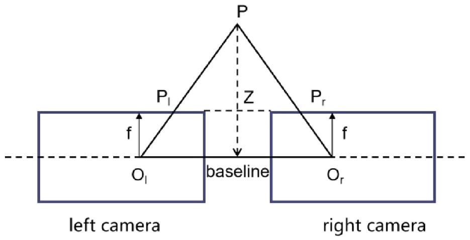
Binocular distance measurement schematic.
The working principle of the trinocular camera is equivalent to using two binocular stereo-vision systems. They are placed along the same direction and at the same distance, as shown in Figure 13. The trinocular stereo-vision system has a narrow baseline and a wide baseline. The narrow baseline is the line between the left and middle cameras and the wide baseline is the line between the left and right cameras. The narrow baseline increases the field of view common to both cameras, and the wide baseline has a larger maximum field of view at each visible distance. 150 The three cameras of the trinocular stereo vision system take three terrain images from different angles and then use the stereo vision matching algorithm to obtain the depth information of the terrain.
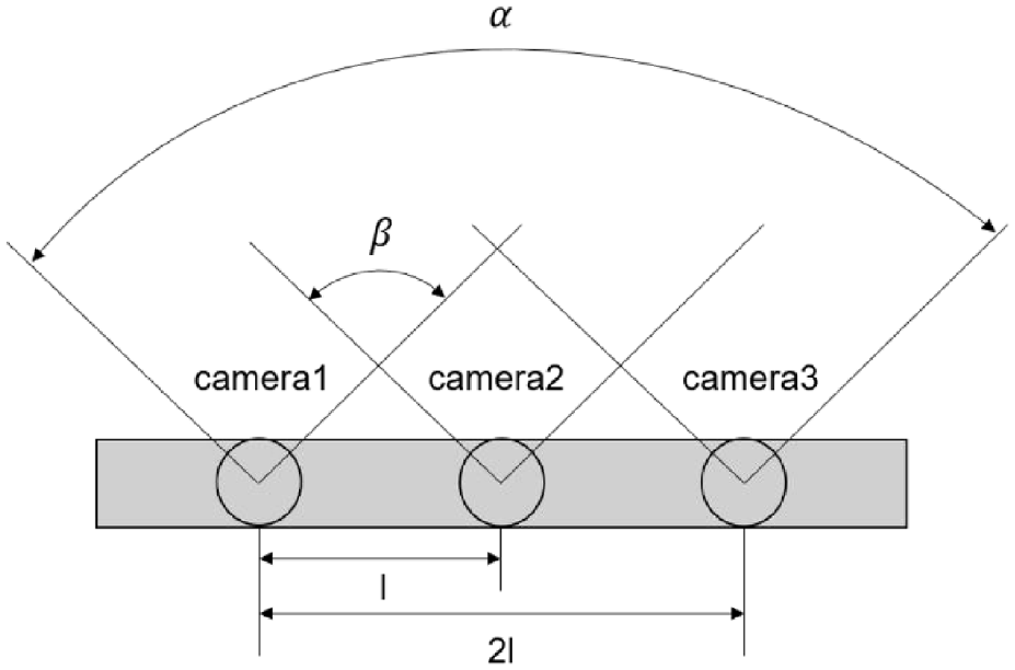
Schematic diagram of the trinocular camera, where α is the maximum field of view of the left and right cameras, and β is the common field of view of the left-center camera.
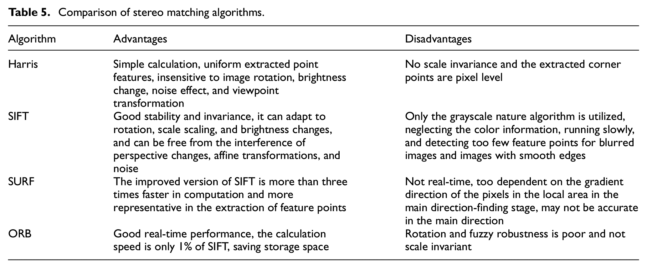
Similar to monocular, stereo ranging works on the principle of affine transformation of the actual object as it is captured by the camera into the picture. The process includes calibration of the camera, stereo correction of the image, calculation of the parallax map, and calculation of the depth map. Due to parallax, the stereo vision system requires stereo matching of the corresponding points captured in different images. Stereo matching is mainly divided into global matching and local matching. The global approach is to consider the parallax assignment as a global energy function minimization problem for all parallax values, which requires constraints on the scan line and even the whole map. Therefore, although global matching has high accuracy and better robustness, the computation speed is slow and cannot meet the real-time requirements. In contrast, the local method only constrains small areas around pixels with low computational complexity and short running time, so local matching is mainly applied to vehicles. In Hou et al., 151 Zhang et al. 152 the vehicle distance measurement is achieved using the center point coordinates based on matching the feature points of the vehicle marker and the license plate, respectively. Li 153 improved the matching speed and accuracy by extracting the Harris corner points of 3D images as feature points and using the wavelet transform sublinear matching method. Still, it does not have scale invariance and is only applicable to close-range vehicle distance measurement due to the weak interference immunity of Harris. Shao et al. 154 proposed a binocular stereo vision calibration method based on parallel optical axes. Its binocular visual obstacle detection matching is achieved by matching left and right images using the SIFT algorithm. The SIFT feature points can maintain good invariance when the scale size of the image changes or when the image is rotated or panned and still maintain certain stability when the light intensity and the angle of the camera change, thus avoiding certain noise interference. Pan and Wu 155 is positioned by combining with high-precision maps. The current road information is obtained by stereo vision camera, and preliminary mapping of position is performed by using Kalman filter to match with map road marking information. By using the ORB algorithm (Oriented FAST and Rotated BRIEF) for feature point matching left and right eye and front and back frame to extract the consistency information in the image sequence, the position change of consistency information in the image sequence is selected for camera motion estimation. Thus the camera pose is derived from achieving ranging. However, due to the large number and uneven distribution of feature points extracted by the traditional ORB algorithm, the accuracy of this stereo-depth estimation method is low. In Huang et al., 156 a vehicle distance measurement method based on machine learning and an improved ORB algorithm is proposed. The method uses dynamic thresholding to improve the quality of feature point extraction and the Progressive Sample Consensus (PROSAC) algorithm in the feature matching stage to reduce mismatching to improve the front vehicle distance measurement accuracy. Wei et al. 157 proposed the concept of SurroundDepth. The depth map between cameras is obtained by processing multiple surrounding views and fusing the information from multiple views with a cross-view transformer. The comparison of several stereo matching algorithms is shown in Table 5.
Comparison of stereo matching algorithms.
Deep learning-based stereo depth estimation
Traditional stereo-based depth estimation is achieved by matching the features of multiple images. Despite extensive research, it still suffers from poor accuracy when dealing with occlusion, featureless regions, or highly textured regions with repeating patterns. 158 In addition, the process of finding matching points is computationally complex, and the matching process also involves setting appropriate window parameters for matching data. In recent years, stereo depth estimation based on deep learning has developed rapidly, and the robustness of depth estimation has been greatly improved by using prior knowledge to characterize features as a learning task.
All algorithms for stereo depth estimation are to get more accurate depth and parallax maps. In 2016, Žbontar and LeCun 159 proposed MC-CNN to construct a training set by labeling data. A positive sample and a negative sample are generated at each pixel point, where the positive samples are from two image blocks with the same depth, and the negative samples are from image blocks with different depths, and then the neural network is trained to predict the depth. However, its computation relies on local image blocks, which introduces large errors in some regions with less texture or recurrence of patterns. Therefore, in 2017 Kendall et al. 160 proposed GC-Net, which performs multilayer convolution and downsampling operations on the left and right images to extract semantic features better, and then uses 3D convolution to process Cost Volumn so as to extract correlation information between the left and right images as well as parallax values. In 2018, Chang and Chen 161 proposed PSMNet, which employs pyramidal structures and null convolution to extract multifractional aspect information and expand the field of perception and multiple stacked HourGlass structures to enhance 3D convolution so that the estimation of parallax relies more on the information at different scales rather than local information at the pixel level. Thus, a more reliable estimate of parallax can be obtained. Yao et al. 162 proposed MVSNet, which utilizes 3D convolutional operation cost volume regularization. It first outputs the probability of each depth. It then finds the weighted average of the depths to obtain the predicted depth information, using reconstruction constraints (photometric and geometric consistencies) between multiple images to select the predicted correct depth information. In 2019, Luo et al. 163 proposedP-MVSNet based on it, which makes a better estimation structure by a hybrid 3D Unet with isotropic and anisotropic 3D convolution. Guo et al. 164 proposed the Group-wise correlation stereo network (GwcNet), which establishes group correlations of cost quantities to improve the performance of the network and reduce the number of parameters. When tested with limited computational costs, their model yielded greater returns than similarly advanced networks. Mauri et al. 165 For the real-time stereo matching problem on high-resolution images Yang et al. 166 proposed HSMNet. This framework runs significantly faster than existing techniques in incremental search for correspondences in a hierarchy from coarse to fine, and is able to predict the depth of close objects accurately in real-time at different scales. However, PSMNet stacked hourglass backbone leads to accuracy loss in parallax maps, Zhang et al. 167 proposed GA-Net including semi-global aggregation layer and local guided aggregation layer. The former aggregates the cost of multiple directions of the whole map, which enables better estimation in occluded areas and low-texture areas, while the latter aggregates local costs to handle finer structures and object edges. Yao et al. 168 proposed an alternative solution, a content-aware inter-scale cost aggregation method. It learns dynamic filter weights based on the content of the left and right views at both scales, and adaptively aggregates and upsamples the cost quantities from coarse to fine scales, which greatly reduces the computational cost. Chabra et al. 169 considering that existing stereo networks (e.g. PSMNet) produce parallax maps that are not geometrically consistent, they propose StereoDRNet, which takes as input geometric errors, photometric errors, and undetermined parallax, to produce depth information and predict the occluded portion. This approach gives better results and significantly reduces computational time. However, these networks use discrete points for depth estimation, thus introducing errors. In 2020, Garg et al. 170 proposed a CDN for continuous depth estimation. In addition to the distribution of discrete points, the offset at each point is also estimated, and the discrete points and the offset together form a continuous parallax estimate. For the problem of too much computation and memory consumption of 3D convolution Xu and Zhang 171 proposed AANet and tried to replace 3D convolution with 2D convolution and proposed a sparse points based intra-scale cost aggregation method to obtain parallax maps faster and with higher accuracy. Badki et al. 172 utilizes multiple binary classifiers for parallax estimation so that the accuracy of speed and depth prediction can be balanced on demand. The main limitation of 3D convolution-based stereo matching networks is the slow computational speed, which has been addressed by more previous work using the multiscale idea. In 2021, Tankovich et al. 173 proposed a new approach HITNet to represent parallax as a tile, which on the one hand enables the modeling of tilted parallax planes in the real world, and on the other hand, equips the tile with features enabling it to be tuned step-by-step in a multi-scale network with much lower computational effort. Tosi et al. 174 proposed Stereo Mixture Density Networks (SMD-Nets), which effectively solved the problem of recovering sharp boundaries and high-resolution output. However, for the problem of consuming a large amount of video memory and computation time at high resolution, Yao et al. 175 proposed a decomposition method. The parallax of points in the larger plane of the image can be estimated at low resolution, while additional detailed points are then estimated at high resolution. In this way, dense matching is performed at low resolution and sparse matching is performed at high resolution, thus reducing the computing time.
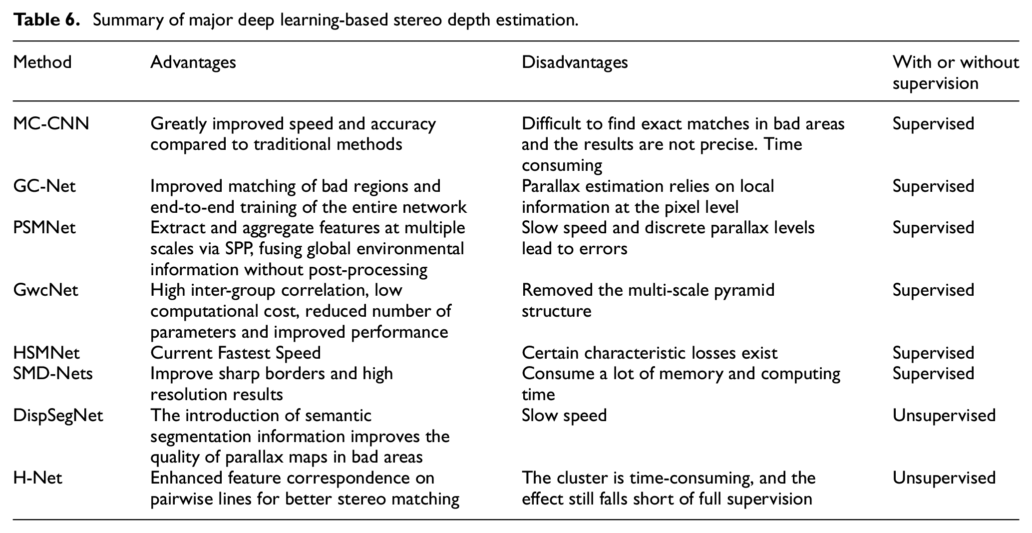
Most of the previous methods rely on fully supervised learning has limitations for complex road conditions, Zhou et al. 176 proposed an unsupervised method that updates network parameters in an iterative manner and learns stereo matching guided by left-right check, but suffers from loss of detail and geometric information. In 2019, Zhang et al. 177 proposed DispSegNet based on CNN with insufficient parallax accuracy in occluded or low-texture regions. They introduced semantic segmentation information for parallax refinement. In addition, this network can output parallax maps and semantic segmentation maps, which is useful in autonomous driving. In 2022, Huang et al. 178 proposed H-Net, which combined epipolar geometry with learning-based depth estimation approaches, incorporating complementary information in stereo image pairs and narrowing the gap with supervised learning. Table 6 summarizes the main several methods for stereo depth estimation based on deep learning.
Summary of major deep learning-based stereo depth estimation.
RGB-D distance measurement
RGB-D camera generally contains three cameras: a color camera, an IR transmitter camera, and an IR receiver camera, and the principle is shown in Figure 14. Compared with stereo cameras, which calculate depth by parallax, RGB-D can actively measure the depth of each pixel. Moreover, 3D reconstruction based on RGB-D sensors is cost-effective and accurate, which makes up for the computational complexity of monocular and stereo vision sensors to estimate depth information and the lack of guaranteed accuracy.
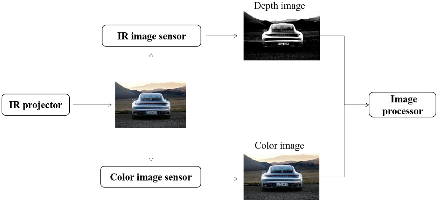
RGB-D schematic.
RGB-D measures the pixel distance, which can be divided into the infrared structured light method and the time-of-flight (TOF) method. The principle of structured light 179 is that an infrared laser emits some patterns with structural features to the surface of an object. Then an infrared camera will collect the pattern variations due to the different depths of the surface. Unlike stereo vision which relies on the feature points of the object itself, the structured light method characterizes the transmitted light source, therefore, the feature points do not change with the scene, which greatly reduces the matching difficulty. According to the different coding strategies, there are temporal coding, spatial coding, and direct coding. The temporal coding method can be classified into binary codes, 180 n-value codes, 181 etc. It has the advantages of easy implementation, high spatial resolution, and high accuracy of 3D measurement, but the measurement process needs to project multiple patterns, so it is only suitable for static scene measurement. Spatial coding method has only one projection pattern, and the code word of each point in the pattern is obtained based on the information of its surrounding neighboring points (e.g. pixel value, color, or geometry). It is suitable for dynamic scene 3D information acquisition, but the loss of spatial neighbor point information in the decoding stage leads to errors and low resolution. Spatial coding is classified into informal coding, 182 De Bruijn sequence-based coding, 183 etc. Direct coding method is performed for each pixel. However, it has a small color difference between neighboring pixels, which will be quite sensitive to noise. It is unsuitable for dynamic scenes, including the gray direct coding proposed by Wong et al. 184 and the color direct coding proposed by Tajima and Iwakawa. 185
TOF calculates the distance of the measured object from the camera by continuously emitting light pulses to the observed object and then receiving the light pulses reflected back from the object and by detecting the time of flight of the light pulses. Depending on the modulation method, it can be generally divided into Pulsed Modulation and Continuous Wave Modulation.
After measuring the depth, RGB-D completes the pairing between depth and color pixels according to the individual camera placement at the time of production and outputs a one-to-one color map and a depth map. The color information and distance information can be read at the same image location, and the 3D camera coordinates of the pixels can be calculated to generate a point cloud. However, RGB-D is susceptible to interference from daylight or infrared light emitted by other sensors, so it cannot be used outdoors. Multiple RGB-Ds can interfere with each other and have some disadvantages in terms of cost and power consumption.
Vision SLAM
SLAM (Simultaneous Location and Mapping) is divided into laser SLAM and visual SLAM. Laser SLAM has some disadvantages, such as lack of color information, high price, and insufficient effective distance. Vision SLAM uses a vision sensor as the only environmental perception sensor. The triangulation algorithm of a single vision sensor or the stereo matching algorithm of multiple vision sensors can calculate the depth information with good accuracy. At the same time, because it contains rich color and texture information and has the advantages of small size, lightweight, and low cost, it has become a current trend of research. Vision SLAM is divided into monocular vision SLAM, stereo vision SLAM, and RGB-D vision SLAM, depending on the vision sensor category.
Monocular vision SLAM
The monocular SLAM is a simple, low cost and easy-to-implement system using a camera as the only external sensor. Monocular vision SLAM is divided into two types according to whether a probabilistic framework is used or not. Monocular vision SLAM based on a probabilistic framework constructs a joint posterior probability density function to describe the spatial locations of camera poses and map features given the control inputs from the initial moment to the current moment and the observed data, and then estimates this probability density function by a recursive Bayesian filtering method, which is currently widely used because of the unknown complexity of SLAM application scenarios. Grisetti et al. 186 proposed an improved SLAM method based on Rao-Blackwellized Particle Filters that decomposes the joint posterior distribution estimation problem of motion paths and maps into the estimation problem of motion paths with example filters and the estimation problem of road signs under known paths. It considers not only the motion of the robot but also the recent observations, thus greatly reducing the uncertainty. In this approach, each particle carries a single map of the environment, but more particles are needed to ensure localization accuracy in complex scenes, which increases the complexity of the algorithm and is more likely to lead to problems such as sample depletion. Yap et al. 187 improved the particle filtering method by marginalizing the position of each particle feature to obtain the probability that the sequence of observations of that feature is used to update the weights of the particles and does not require the feature positions included in the state vector. Consequently, the algorithm’s computational complexity and sample complexity remain low even in feature-dense environments. Davison et al. 188 proposed MonoSLAM based on Extended Kalman Filtering, which achieves real-time and drift-free dynamic performance by building sparse and continuous maps of natural landmarks online and exploiting prior knowledge. However, due to the reduced motion uncertainty, the search area becomes correspondingly smaller. On the other hand, the EKF-SLAM algorithm suffers from high complexity, poor data association problem, and large linearization processing error. Sim et al. 189 proposed FastSLAM, which still uses EKF algorithm to estimate the environmental features, but the computational complexity is greatly reduced by representing the mobile robot’s poses as particles and by decomposing the state estimation into a sampling part and a resolution part. However, its use of the process model of SLAM as a direct importance function for the sampled particles may lead to the problem of particle degradation, which reduces the accuracy of the algorithm. Therefore, FastSLAM2.0 proposed in Montemerlo et al. 190 uses EKF algorithm to recursively estimate the mobile robot poses, obtain the estimated mean and variance, and use them to construct a Gaussian distribution function as the importance function. Thus, the particle degradation problem is solved. For monocular vision SLAM with the non-probabilistic framework, Klein and Murray 191 proposed a keyframe-based monocular vision SLAM system PTAM. The system utilizes one thread to track the camera pose and another thread to bundle and adjust the keyframe data as well as the spatial positions of all feature points. The dual-threaded parallelism ensures both the accuracy of the algorithm and the efficiency of the computation. Mur-Artal et al. 192 proposed ORB-SLAM based on PTAM with the addition of a third parallel thread, the loopback detection thread, and the loopback detection algorithm can reduce the cumulative error generated by the SLAM system. And because of the rotation and scale invariance of ORB features, the endogenous consistency and good robustness in each step are ensured. A comparison of the two is shown in Figure 15. Mur-Artal and Tardos, 193 Campos et al. 194 proposed ORB-SLAM2 and ORB-SLAM3 and extended them to binoculars, RGB-D, and fisheye cameras. Mouragnon et al. 195 utilized a fixed number of images recently captured by the camera as key frames for local bundle adjustment optimization to achieve SLAM. Bruno and Colombini 196 presents LIFT-SLAM, which combines deep learning-based feature descriptors with a traditional geometry-based system. Features are extracted from images using CNNs, which provide more accurate matching based on the features obtained from learning.
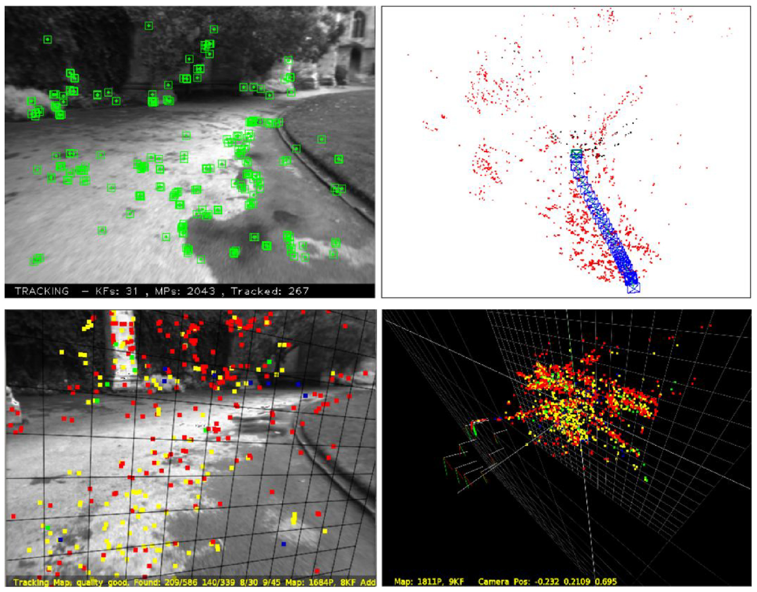
Compared with ORB-slam (top) and PTAM (bottom) initialization maps, the method of the fundamental matrix can explain more complex scenes. © 2015 IEEE. Reprinted, with permission, from Mur-Artal et al. 192
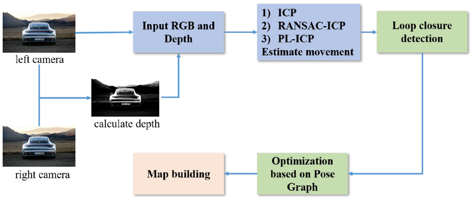
RGB-D SLAM flow chart, depth map obtained from left and right camera images, then motion estimation and scene building by various algorithms at the front end, loopback detection and optimization at the back end.
In general, since monocular SLAM cannot determine the true scale only by image, there are scale uncertainty and scale drift. A relatively good solution at the moment is the fusion of visual and IMUs. IMU can measure angular velocity and acceleration of high frame rate. Especially, when the camera moves too fast, motion blur will occur or the overlap area between two frames is too small for feature matching. Therefore, IMU is a good supplement to visual information and can provide a better pose estimation when the camera moves too fast. In addition, the scale can also be used as an optimization variable in the back-end optimization to reduce the scale drift problem.
Stereo vision SLAM
Stereo vision SLAM uses multiple cameras as sensors. Since the absolute depth is unknown, monocular SLAM cannot get the true size of the motion trajectory and map. Stereo can calculate the true 3D coordinates of the landmarks in the scene simply and accurately through the parallax. However, it requires higher accuracy of calibration parameters and is costly. In Engel et al., 197 the proposed LSD-SLAM by fixing the baseline can avoid the scale drift that usually occurs in monocular SLAM, and in addition, by combining two parallax sources can estimate the depth of the under-constrained pixels. ORB-SLAM2 applied to stereo vision SLAM uses dual threads to extract ORB feature points for the left and right images, and then computes binocular seeing feature points and performs matching. Liu et al. 198 proposes DMS-SLAM based on ORB-SLAM 2.0 using sliding window and grid-based motion statistics (GMS) feature matching methods to find static feature locations with some improvement in execution speed. However, point feature-based algorithms do not work well in low-texture environments, so Gomez-Ojeda et al. 199 proposes PL-SLAM combining point and line features based on ORB-SLAM2 and LSD, which can guarantee robust performance in a wider range of scenarios. Bultmann et al. 200 proposed a framework for stereo vision Dual Quaternion Visual SLAM. It uses a Bayesian framework for pose estimation, and for point clouds and optical flow of the map, DQV-SLAM uses an ORB function to achieve reliable data correlation in a dynamic environment. The performance is better compared to filter-based methods. Cvišić et al. 201 proposed SOFT, a stereo vision odometry computation based on feature tracking. SLAM is achieved by bit pose estimation and construction of feature point-based bit pose maps, and the global consistency of the system is guaranteed compared to monocular ORB. However, the binocular camera degrades to a monocular when the target is far away. Therefore, a large amount of research has been conducted around monocular ORB in recent years.
RGB-D vision SLAM
RGB-D vision SLAM uses an RGB-D sensor as the image input device. This sensor integrates a color camera and an infrared camera to capture both color images and the corresponding depth images and thus is gradually becoming the trend of SLAM. Henry et al. 202 extracted feature points from RGB images and then combined them with depth information to inverse map the feature points to 3D space and then optimized the initial poses using ICP which is a point cloud matching algorithm. However, the RGB-D data often lacks validity when in an environment with changing light intensity, so there is now a fusion of it with the state increments calculated by the IMU sensor 203 to obtain better results. The current deep SLAM consists of two parts, the front end, and the back end. The front-end estimates camera motion from images between adjacent frames and recovers the spatial structure of the scene, while the back-end receives the camera pose output from the visual odometry at different moments, as well as information from loopback detection, and optimizes them to obtain globally consistent trajectories and maps. Newcombe et al. 204 used Kinect RGB-D for 3D environment reconstruction. KinectFusion technology can add every frame of acquired image data to the 3D map in real time. Still, it requires high hardware configuration because it occupies huge memory space, and the performance of SLAM deteriorates for a long time. Endres et al. 205 proposed improvement and optimization of the RGB-D SLAM problem based on it. The front-end of the system extracts features from the RGB image of each frame, combines both RANSAC and ICP algorithms to obtain motion estimates, and uses EMM (Environment Measurement Model) model to validate the motion estimates. The back end builds a map based on pose graph optimization.
Conclusion
With the rapid development of autonomous driving technology, environmental perception is the basis and prerequisite for vehicles to realize autonomous driving. Through the acquisition, processing, and analysis of environmental images, it finally gets the information about the road, pedestrians, and obstacles around the vehicle and then makes decisions and controls.
In this paper, the application of vision technology in the field of autonomous driving is described in a systematic way. In the field of object detection and identification, traditional methods first preprocess the acquired images, including image compression, image enhancement and recovery, and image segmentation. Then, the edge features, appearance features, statistical features, transformation coefficient features, and other features of the images are compared with existing patterns to determine their categories. Image detection and identification technology combined with deep learning needs more time in training. However, its reliability and processing speed are better, so it has become the future trend of object identification, and this paper introduces and compares the networks and algorithms for image processing. Currently, the mainstream recognition algorithms include the RCNN series, YOLO series, FCN, and SSD, etc. Faster R-CNN has higher accuracy mAP and lower miss detection rate but slower speed. On the contrary, SSD balances the advantages and disadvantages of YOLO and Faster RCNN with better accuracy and speed. For the problem of blind spot detection, the Around View Camera can stitch together the images from all directions on top of the car to effectively avoid blind spots and greatly reduce traffic accidents. Its key technologies include image correction, top view transformation, and image stitching.
In depth estimation, the monocular camera dominates a large market with its advantages of low cost and fast detection. Its measurement methods mainly include the geometric relationship method, data regression modeling method, inverse perspective transformation method, SFM based method and so on. This paper also compares the principles and advantages, and disadvantages of different SFMs, among which hybrid SFM combines the advantages of incremental and global styles with better results. For deep learning based monocular depth estimation, this paper introduces and compares some algorithms, including supervised methods based on classification, regression, conditional random fields, and unsupervised methods based on stereo images and video sequences. Stereo cameras directly perform distance measurements through parallax, although they do not rely on sample datasets. However, camera calibration and fusion are required, and the commonly used algorithms are SIFT, SUFT, and ORB. As for monocular, it can obtain the complete 3D information of the road for the recognition of road information, thus providing a reference for decision-making modules such as obstacle avoidance and path planning. And by experimental tests, 165 the stereo method has a higher accuracy than the single-purpose based method. In contrast, since RGB-D does not depend on the fixed characteristics of the object itself, it can actively measure the depth of each pixel with high accuracy through infrared transmitting and receiving devices.
Visual SLAM has become a current research trend with its advantages of rich color and texture information, small size, lightweight, low cost, and real-time. The monocular visual SLAM has a simple structure. Among them, the probabilistic framework-based approach describes the spatial location of camera poses and map features by constructing a joint posterior probability density function, which is better adapted for unknown environments. The stereo vision SLAM can simply and accurately calculate the true 3D coordinates of the landmark points in the scene through the view source difference and can estimate the depth of the under-constrained pixels. RGB-D vision SLAM consists of image processing front-end and back-end optimization, where the front-end extracts features from each RGB image frame and performs motion estimation. The back end optimizes and builds real-time maps based on pose graphs.
Future outlook
Visual perception performance
Although we have advanced vision sensor technologies, there is still the problem of decreasing accuracy in bad weather. Yang 206 experimentally concluded that the detection error reaches 6%−17% in rain and snow, and this error lays a hidden danger for traffic accidents. Therefore, it is the trend to explore new sensor types to replace classical cameras. For example, the event camera proposed in Wu et al., 207 whose pixels can individually detect changes in the logarithm of light intensity and output event information containing position, time, and polarity when the amount of change exceeds a certain threshold, has the advantages of low latency, high dynamic range, and low power consumption. The unique output and operating characteristics make it especially suitable for applications with high speed motion, changing light conditions, and low energy consumption. In addition, the fusion of vision sensors with other sensors, such as IMU and radar, is also a development trend. Exploring new sensor fusion schemes is a good research direction to improve the robustness and accuracy of vision.
For depth estimation, binocular images need to use stereo matching for pixel point correspondence and parallax calculation, so the computational complexity is also higher. Moreover, the matching effect of low texture scenes is not ideal, the main reason is that the feature can not be extracted effectively in the region to calculate the matching error. One solution is to improve the dynamic range of the camera or to use infrared cameras and Radar and Lidar for perceptual fusion. Monocular depth image processing relies heavily on large-scale labeled datasets and is less effective for unknown unlabeled target recognition. Hence, unsupervised learning techniques are still a future research direction. Furthermore, the depth estimation error increases with distance. Because it is difficult to distinguish the pixels of discrete images for long distances, and the recognition and ranging of objects in the case of multiple vehicles and mutual occlusion between vehicles in road driving will also be affected. Therefore, long-distance ranging in complex scenes will continue to be a hot topic for future research. One improvement method is to increase the range of parallax by increasing the spatial resolution of the image or increasing the baseline length. For the reduction of errors in the background, the current trend is to calculate element values and compare them with thresholds by semantic segmentation or combine them with geometric priors for estimation, and input the current state of the camera acquisition and the future distribution in training into a convolutional network for inference. Supervised networks can use supervised signals with high-level semantic information and post-process with the results of object detection and semantic segmentation to better understand the scene.
In addition, most current detection algorithms are still static graph detection, while video data as well as other data support more and more categories, and detection techniques in this area also need to continue to develop. Object detection based on video timing continuity and pixel-level instance detection will be the key breakthrough direction in the future.
High speed and network lightweighting
For autonomous driving, real-time is very important. Therefore, fast image segmentation is needed for the purpose of fast Region of Interest (ROI) recognition. In the future development, the processing speed needs to be further improved. Currently, methods for identifying distance measurements usually rely on highly parameterized deep neural networks to achieve high accuracy. This implies the huge number of parameters and slow inference speed of the model. For the efficiency problem, the usual approach is to perform model compression, that is, compression on an already trained model that makes the network carry fewer network parameters, thus solving the memory and speed problems. Compared to processing on the already trained model, lightweight model model design is more reasonable, for example, SqueezeNet proposed by Iandola et al. 208 makes the network parameters reduced with more efficient network computation without losing network performance. Therefore, lightweight networks become the future trend.
Visual SLAM
In the past decades, visual SLAM has developed rapidly and is used in the field of autonomous driving, and is very good at perception and localization tasks. However, the current visual SLAM still suffers from the problems of difficulty in balancing real-time and accuracy, sensitivity to light, and low robustness in poor lighting conditions or complex lighting situations. At the same time, the application in outdoor dynamic and complex scenes still faces great challenges. As a crucial step in SLAM systems, loop-back detection has achieved good results in terms of accuracy and loopback rate, but there are still problems such as excessive manual intervention, low robustness, and long training time. Therefore, using more relevant knowledge, such as deep learning, target recognition, and semantic segmentation, is the future development direction. Using neural networks can better extract semantic information and improve the generalization and reconstruction effect of the model. In addition, the projection model on which vision depends also has broad prospects for development. Firstly, the monocular and binocular combination of long and short baselines can not only ensure the level of large-scale positioning, but also improve the accuracy of obstacle detection and map construction in short to medium range. The addition of wide-angle and fisheye cameras can further enhance the coverage of visual SLAM. In the future, the fusion of different types of cameras and multiple sensors can bring greater application space.