
Abstract
Although autonomous vehicles (AV) have been rapidly developed, their control technology is not sufficiently mature for daily use, yet not human-centred enough. Some studies regarding trajectory planning are overly conservative and the vehicle avoids obstacles in an unhuman-like trajectory which causes discomfort to passengers; meanwhile, other studies are overly simplistic, the transport scenario, and vehicle trajectory are disregarded. The potential field (PF) algorithm is one of the most frequently used methods for the trajectory planning of AVs; however, most studies regarding the PF algorithm do not consider driving comfort and smoothness. This paper introduces optimised human-centred dynamic trajectory planning for AVs. The PF algorithm is implemented in a vehicle simulation model, which is integrated with model predictive control (MPC). The reference path is planned by PF algorithm and improved by MPC. The human-centred AV control is proposed in a simulation environment. The proposed planning method achieves a trade-off between safety, driving comfort, and driving smoothness and is validated with several driving simulation scenarios.
Keywords
Introduction
According to the World Health Organisation, 1 1.35 million fatalities caused by road crash accidents occur each year globally. The main reasons for car accidents are overspeeding, drunk driving, seat belt violation, and reaction delays, which are human factors. It has been claimed that human factors involving vehicles and road environments are the most decisive factors in road safety. 2 Implementing autonomous vehicles (AV) is one of the most effective methods to improve road safety.
The UK government had claimed that fully AVs will be driven on roads in 2021. Tesla 3 has completed 3 billion miles of road tests with Autopilot engaged, Waymo 4 has traversed over 20 million miles in the USA, and Baidu has completed over 1 million miles of road tests in China. 5 Although it has been claimed that we are moving towards the advanced trials of self-driving vehicles, the control of AV has not been fully established for daily use. 6 Some of the current studies are overly conservative and causes the vehicle to avoid obstacles in an unhuman-like way, whereas others are overly simplistic and causes the vehicle trajectory to be disregarded. Herein, an optimised human-centred dynamic trajectory plan for AVs is introduced.
Each AV comprises three layers (see Figure 1). The main objective of this study is trajectory planning in the control layer. In some literature, motion planning includes trajectory planning and path planning, while in other literature, motion planning is equivalent to trajectory planning. In this study, the second definition is used. Path planning is not investigated in this study. For the perception layer, it is assumed that the detection range of AVs is 150 m. The kinematic bicycle model is used as the vehicle dynamics model for the execution layer.
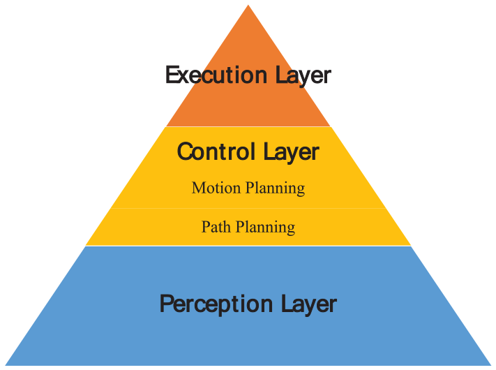
Layer structure of autonomous vehicle.
The main function of trajectory planning is to avoid obstacles, change lanes safely and merge into lanes. Trajectory planning is based on physics and mathematics models. Unlike path planning, trajectory planning is a sequence of movements. It is not only a calculation but also the co-operation of different systems, including sensors, such as computer vision, and actuators, such as steering actuator. Many trajectory planning algorithms exist, including function optimisation (for example, potential field method), rapidly exploring random tree, grid-based search and probabilistic roadmap.7–9
Since the potential field (PF) algorithm has a smaller computational complexity than other algorithms and it considers other factors in the traffic environment, it is more suitable for modern AV control. 10 With recent development of computer vision and sensors, PF algorithms have become easier to implement, and the precision of the PF method has increased.
Studies regarding the PF method trajectory planning of AVs are abundant. For example, the PF algorithm and neural network algorithm were used to build a human-centred decision-making system for steering control. 11 The trajectory planning was decided by the network. The MPC was used to perform trajectory replanning based on the safe distance-based threat assessment strategy. 12 The algorithm used the precise position of the ego vehicle to calculate the precise distance of each wheel to the obstacle; subsequently, the MPC was used to output the steering angle to steer the ego vehicle to the target position, where the distance to the obstacle was larger than the safety distance. PF combining nonlinear MPC control was also used in trajectory planning. 12 However, these studies did not consider other road users or infrastructure.
A PF model for all road users in the road system has been established, 13 where the trajectory planning was made based on the safety of the traffic system, however, the vehicle dynamics was neglected. In particular, a dynamic trajectory planning algorithm based on the PF algorithm was introduced, 14 in which vehicle dynamics and road structure were considered. The potential of the road was the sum of crossable and uncrossable obstacles and road lane boundaries. The future state of dynamic obstacles was also predicted. However, vehicle was the only considered obstacle in the study; therefore, the number of simulation scenarios was insufficient for evaluating the availability of the model. The PF algorithm and model predictive control (MPC) were used to develop an optimised trajectory plan in scenarios involving a parking vehicle and a pedestrian darting on road. 15 Potential field algorithm and MPC have also been used to plan path for autonomous vehicle. 16 However, in the research, only path planning and collision avoidance were considered, only moving vehicle was considered as obstacles, neither infrastructure nor other transport mobilities were considered. Human-centred trajectory was not considered. PF and MPC have been also used to control the autonomous vehicle platoon. 17 But as prior studies, comfort of trajectory was not considered. While the algorithm was applied to improve an automatic emergency braking system, the driving smoothness and driving comfort were ignored. A trajectory planning method such as the Stanley vehicle in the Defence Advanced Research Projects Agency challenge was designed using the local search algorithm. 18 The cost function of driver comfort and driving consistency was evaluated to select the best path from the candidate paths.
In these previous studies, some research considered collision avoidance, some considered drivers’ comfort and drive consistency, some took transport scenario into consideration, whereas others considered vehicle dynamics; however, none of them included all transport factors and include human-centred trajectory. In this study, the PF algorithm, which is relatively less complex, was used to create a ‘risk map’. Owing to the development of sensors and V2X systems, it is more feasible to use the PF algorithm to generate a reference path. Not only vehicles, but also pedestrian and cyclists are considered as obstacles. Infrastructure is also considered in the PF map establishment. The MPC can be implemented to optimise the trajectory in real-time. In most AV studies, trajectory planning is based on the safety of vehicles, whereas both the comfort of drivers and the driving smoothness were considered in this study to make the trajectory more human-like and human-centred. Moreover, wet and icy road surface are also considered to assess the control algorithm.
This study was organised as shown in Figure 2. The road environment, as well as the vehicle dynamics model and trajectory plan were established in MATLAB/Simulink software. Subsequently, a PF map was developed based on road information; a safe route with the minimum PF was automatically generated according to the map. The MPC controller was developed to optimise the route based on the vehicle dynamics model; subsequently, the most human-centred route was generated within the drivable corridor along the safe route.
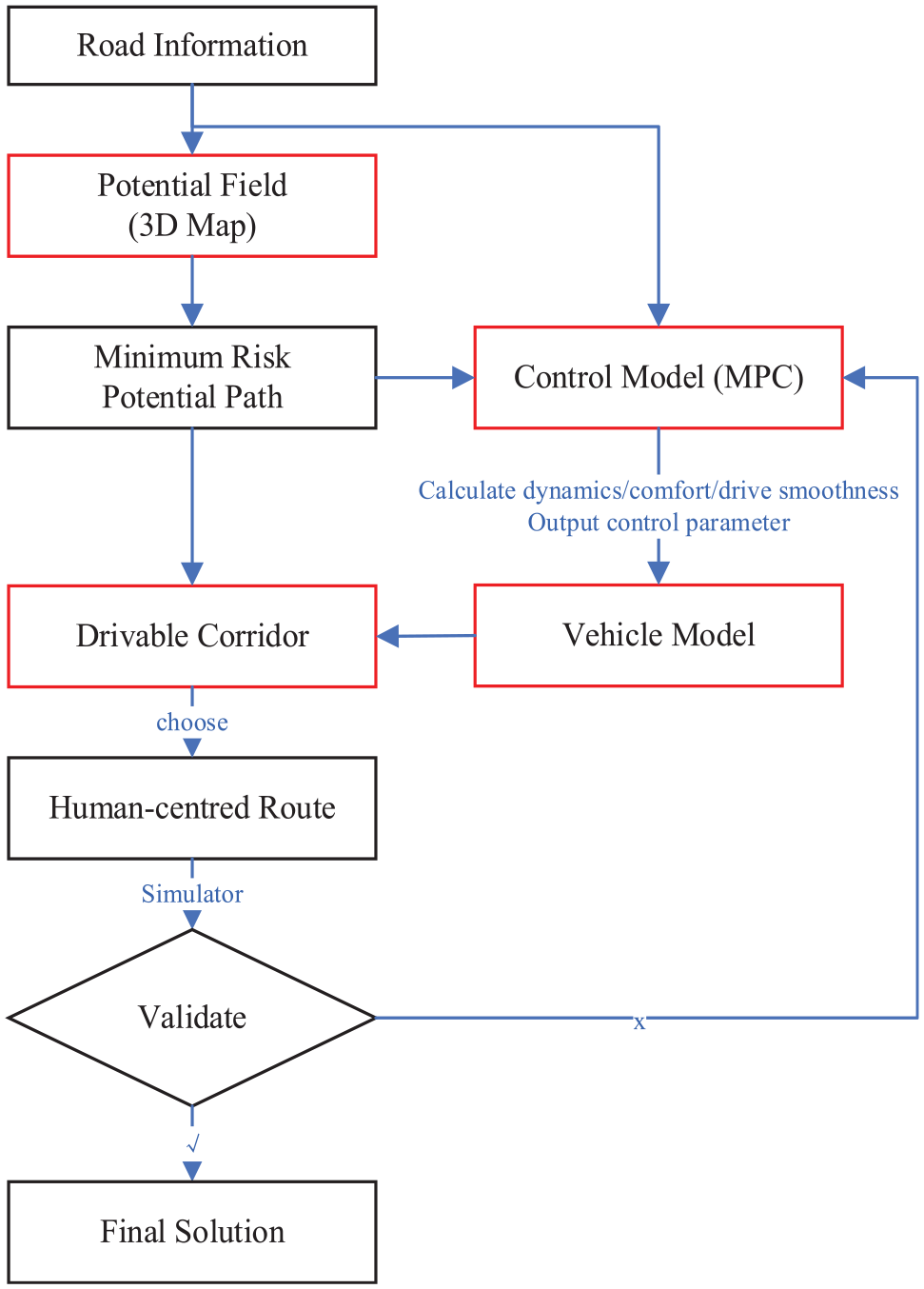
Overall architecture of trajectory planning.
System overview
The bicycle model (see Figure 3) was used as the basic vehicle dynamics model, where v represents the vehicle velocity,
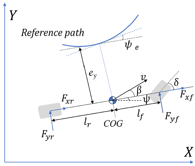
Simplified kinematic bicycle model in global coordinate system for vehicle dynamic control.
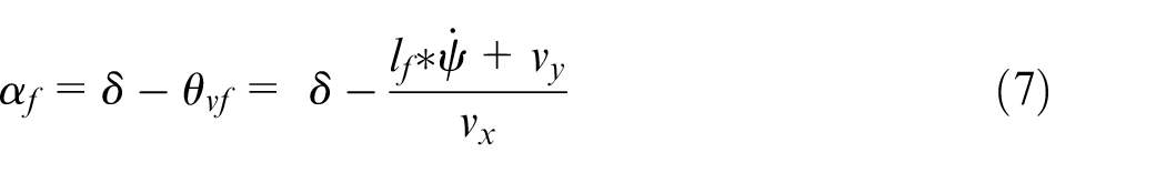
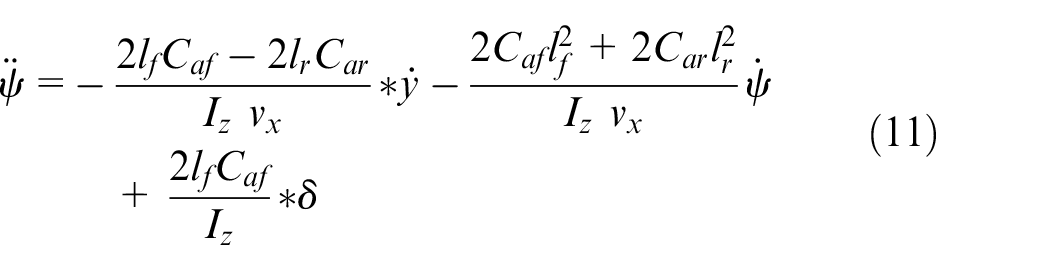
In the lateral direction,


where


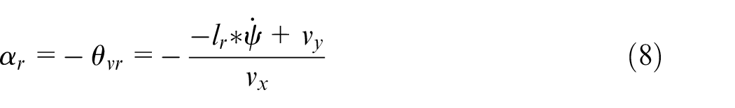
where
According to (1)–(8),
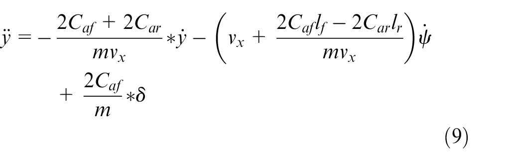

where


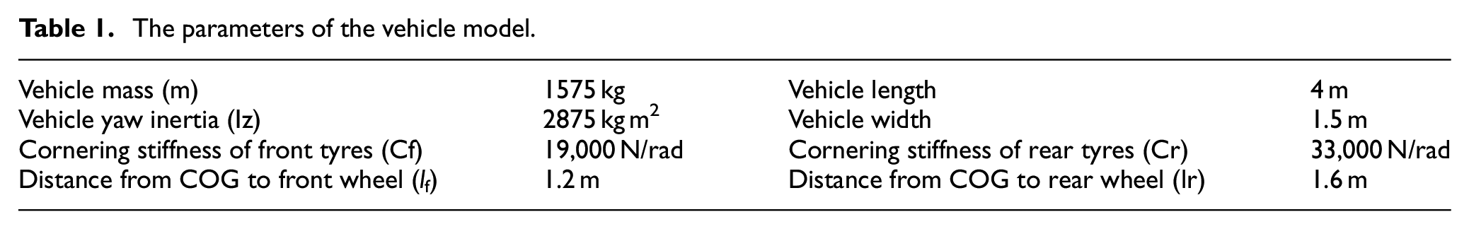
The parameters of the vehicle model.
Base frame of the trajectory planning
The trajectory planning in this study is based on the following principles: the PF risk map was built according to the surrounding environment of the ego vehicle. The safest route was automatically generated according to the risk map, connecting minimum PF points in the driving direction. Subsequently, the MPC optimised the routine balancing safety, driving comfort and driving smoothness (see Figure 4).
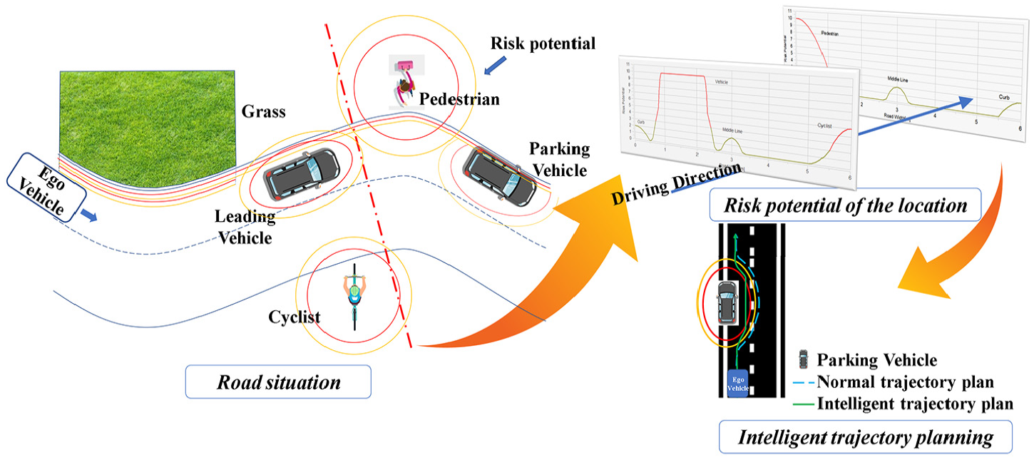
Potential field of the traffic environment and intelligent trajectory planning.
Potential field
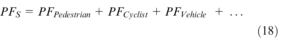
According to its definition in the literature, the PF in this study is expressed as follows:

where
The PF of the road should contain a function that pushes the ego vehicle to drive in its driving lane (3.65 m in width); hence, once the ego vehicle drives out of the lane, it should have the potential to push it back to the original lane. Hence, the PF of the road shown in Figure 5 was adopted. The line y = 1.825 m is the centre line of the driving lane of the ego vehicle and includes the minimum PF of the road.

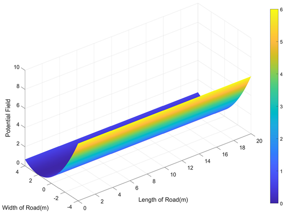
PF of road in this study (UK road).
where (x, y) indicates the position of the ego vehicle. The x-axis is parallel to the driving direction.
In addition to the PFs of the roads, a PF exists for infrastructures along the side of the road. According to prior study, 20 a risk-based corridor exists according to the risk element surrounding the roadside. The PF of a certain infrastructure can be defined. Using grass on the roadsides, for example, the PF function of the infrastructure is defined as in (17) (see Figure 6).
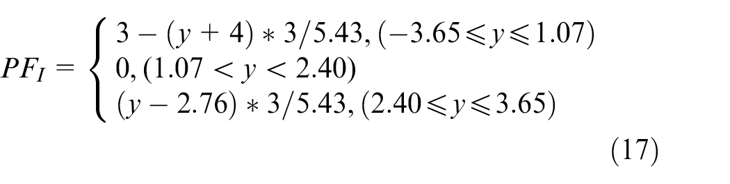
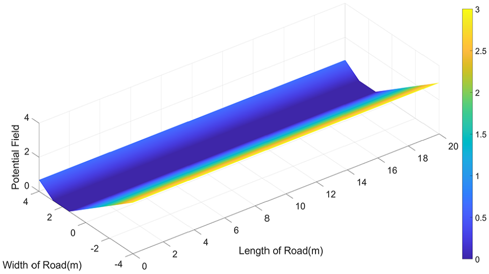
PF of infrastructure (grass) on roadside.
The static (nonmoving) obstacles on the street include pedestrians, cyclists, traffic barriers, and nonmoving vehicles. Static obstacles were primarily studied in most previous studies.13,14,18 The PF of a traffic environment in this study is defined in (18).
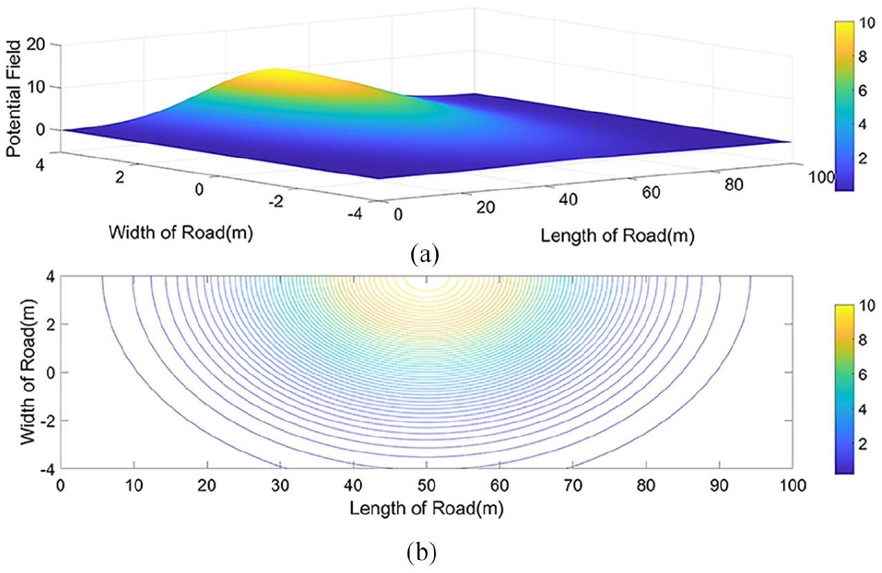
which is similar to the theory in prior study 14 ; the PF should be summed up to calculate the potential risk of the ego vehicle. However, the PFs of the pedestrian and cyclists differ from those of the vehicles. The PFs of pedestrians and cyclists were set to a circle of large radius to ensure that the pedestrian in the centre of the PF is safe.
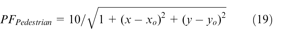
where (
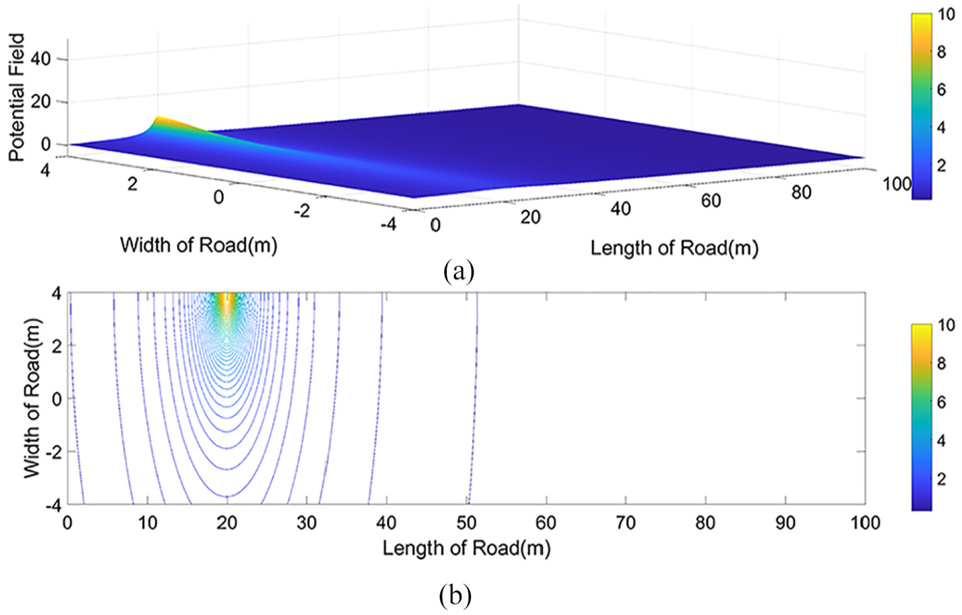
PF of pedestrian: (a) 3D PF map and (b) contour of PF.
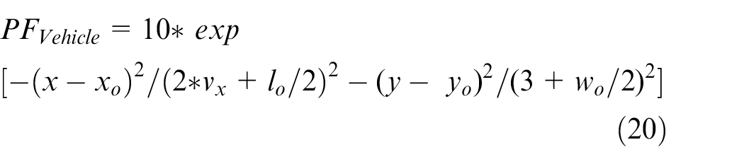
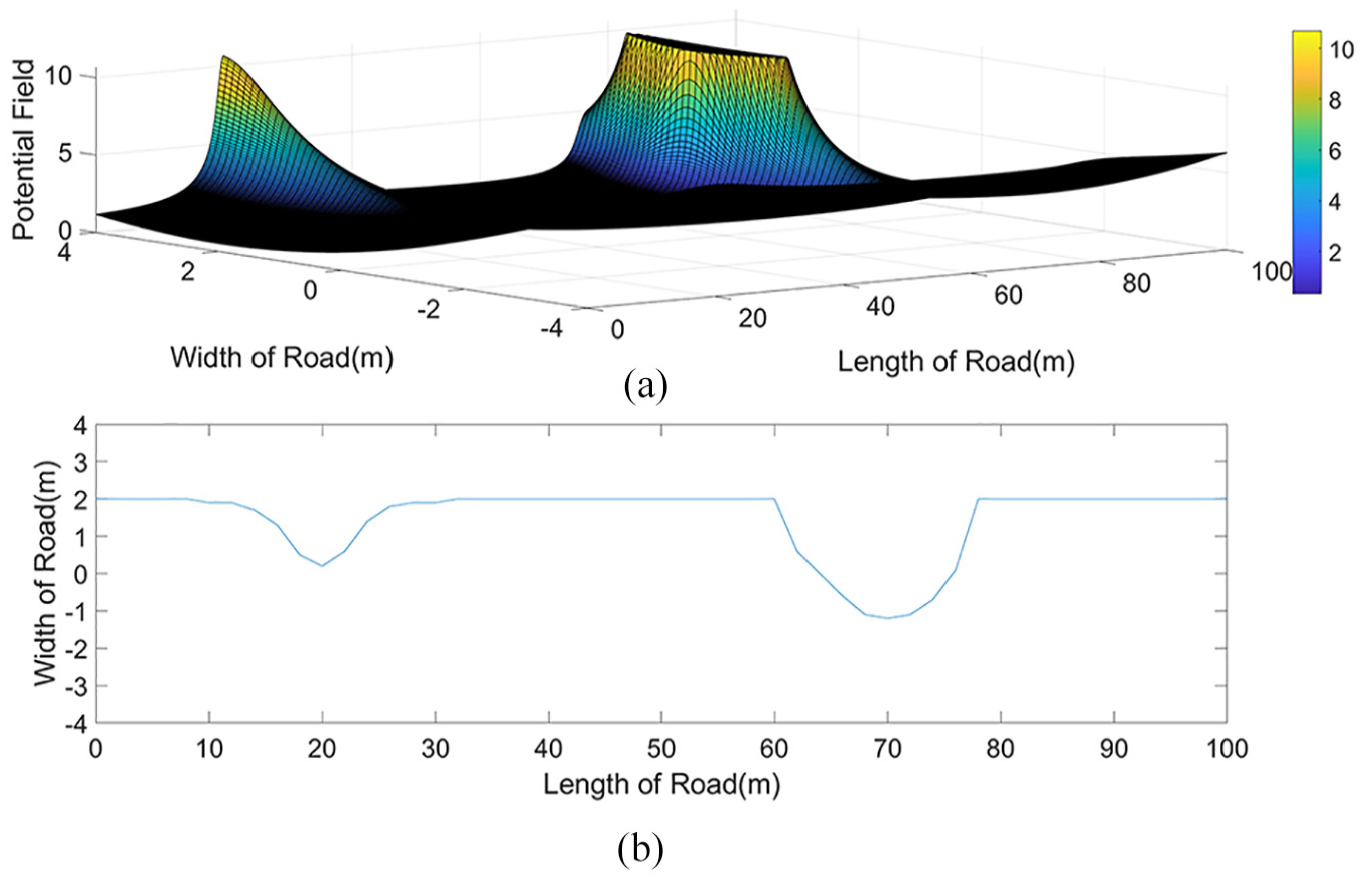
For the PF of vehicles, the longitudinal distance was set to be larger than the lateral distance (see Figure 8). Moreover, the PF of a vehicle has a 150 m range of influence.
PF of static vehicle obstacle: (a) 3D PF map and (b) contour of PF.
where
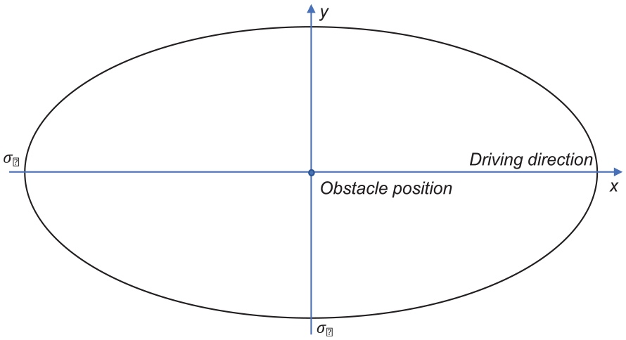
Ellipse shape PF of obstacle vehicles.
Most of the drivers can finish the emergency operation 2 s before a collision occurs. 23 Therefore, the time to collision was set as 2, and the deviation on the longitudinal direction was set to 10 m/s × 2 s = 20 m.
Meanwhile, the lateral deviation was defined as the ego vehicle’s width. 23 However, it was insufficient for collision avoidance, in particular when driving at a high speed. In prior literature, 24 the lateral deviation was set to 3 m when the initial vehicle speed was 10 m/s.
The parameters must be adjusted because the size of the obstacle vehicles varies.
22
The PF formula should be safe for every type of obstacle vehicle. In this case, the
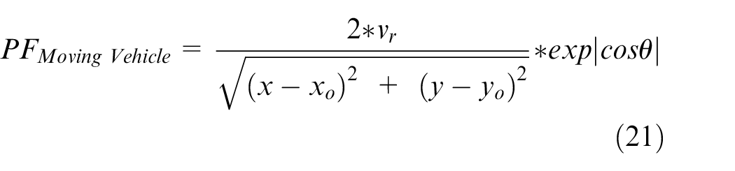
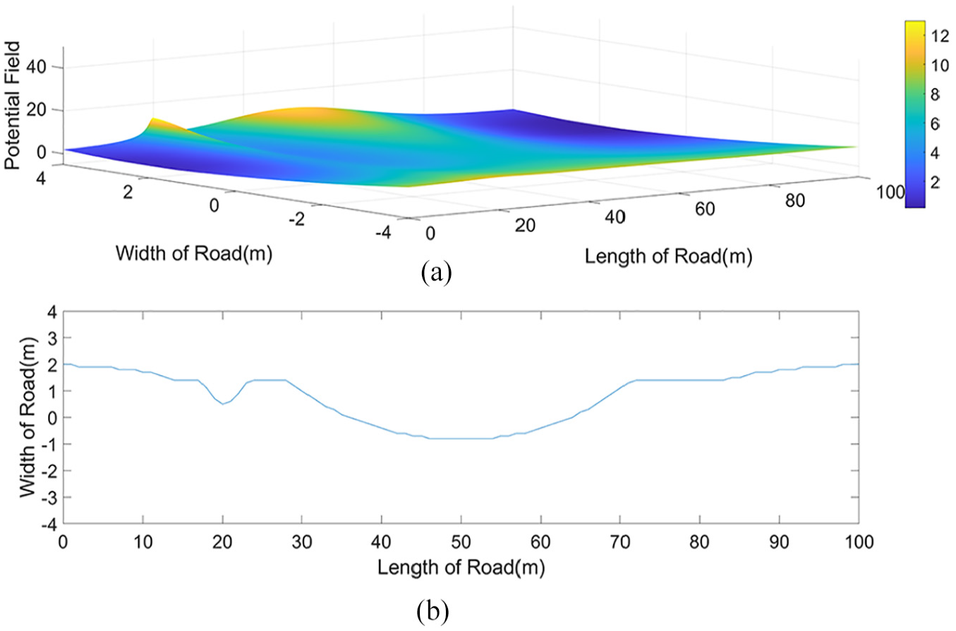
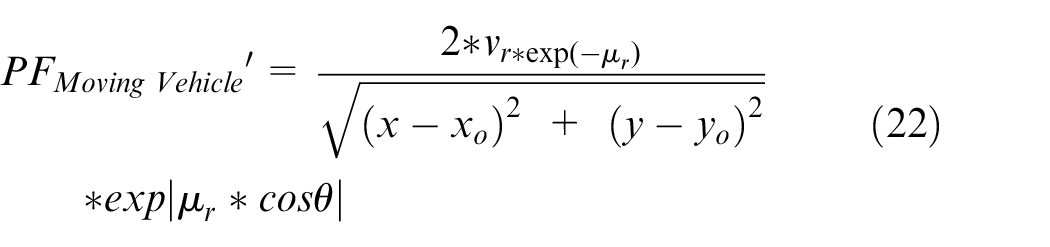
If the obstacles are moving, their risk is higher. The dynamic obstacle should have a different PF shape. 13 The PF of the moving obstacles are related to the relative speed between the obstacles and the ego vehicle as well as the distance from the obstacle to the ego vehicle (see Figure 10). In this study, the PF of a dynamic obstacle is defined as follows:
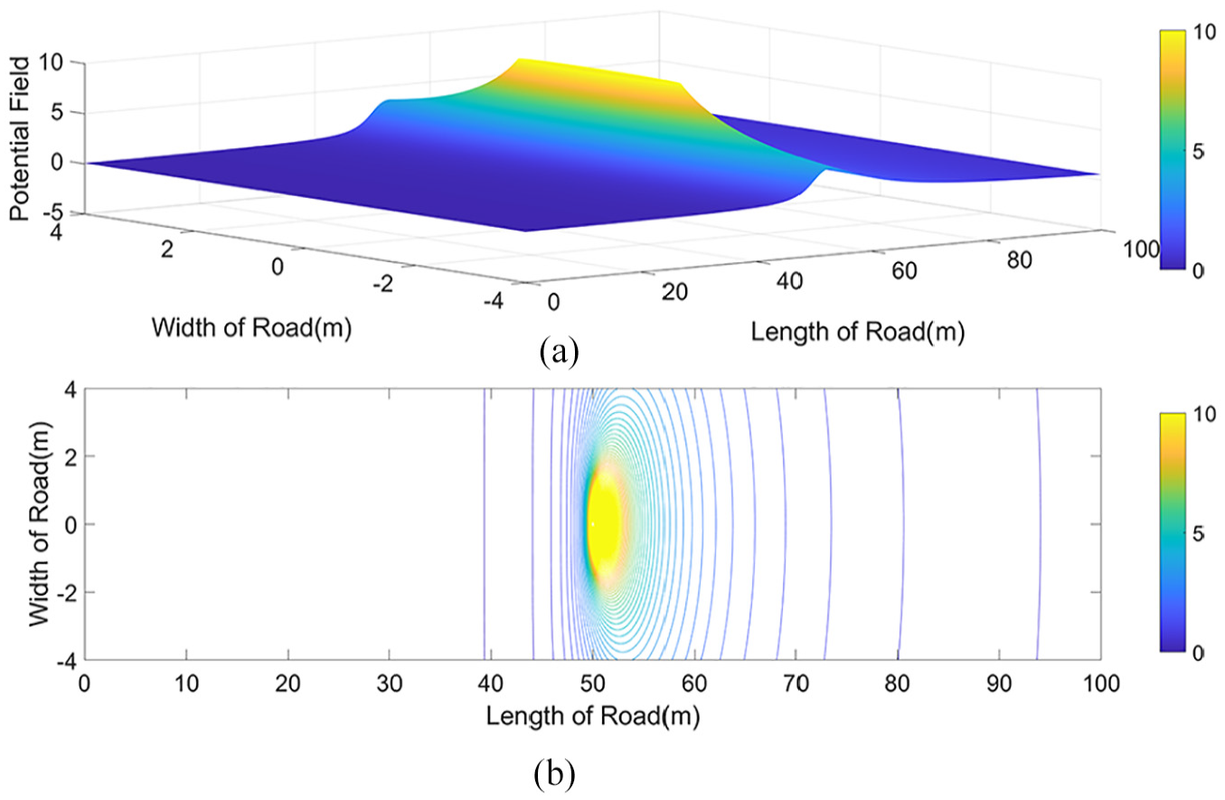
PF of moving vehicle: (a) 3D PF map and (b) contour of PF.
where
After a three-dimensional PF map was established, the safe route was automatically generated by connecting all the minimum PF points along the drive direction (see Figure 11).
Safe route generated from PF map of simulation traffic environment with static obstacles: (a) 3D PF map and (b) safe route.
The nonmoving pedestrian (see Figure 12) was standing at position (20, 3.65), and the moving obstacle was moving from (50, 1.825) at the speed of 5 m/s. The ego vehicle was moving from (0, 1.825) at the speed of 20 m/s and then returned to the centre line of the driving lane at (74, 1.825) after 3.7 s.
Safe route generated from PF map of simulation traffic environment with dynamic obstacle: (a) 3D PF map and (b) safe route.
For the scenarios on extreme road surface, for example, wet or icy road, the PF function of moving obstacle vehicle is related to the adhesion coefficient (
MPC controller
MPC controller has the following cost function:
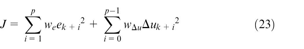
where
In the MPC controller, three key variables exist: system state vector X, manipulate variable U and state output vector Y. The functions of the model inputs and outputs are shown in (24) and (26).


The steering angle was calculated using the MPC controller. The vehicle speed was constant in this study. The vehicle state is the variable that can be directly calculated through matrices. It was calculated after the input variables were transferred to the plant model. In the normal MPC controller model, the vehicle state is a vector that contains the longitude, lateral speed, yaw angle, yaw rate, and lateral velocity, displacement, deviation of lateral displacement, deviation of yaw angle (see (24)).
In (25), dX indicates the derivative of state variables. Using this module, the vehicle state vector can be calculated. The output variables were calculated by the vehicle state and then transferred to the updated model and MPC controller for the next time step simulation (See Figure 13).
The output of the MPC controller’s plant model is as follows:

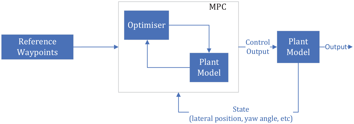
MPC model in vehicle simulation model.
The output vector Y is calculated from the state vector. The state vector X varies according to the models and the problems to be solved.

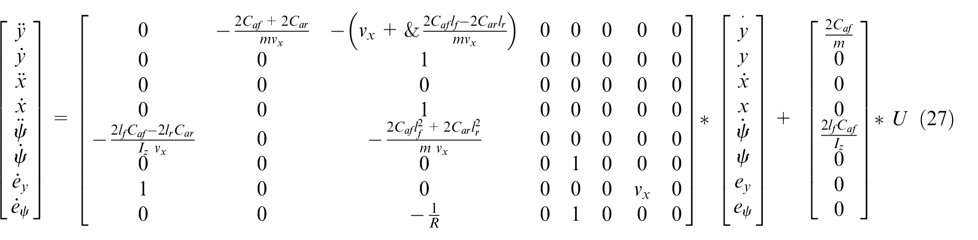
where U is the steering angle. The representing state space is defined as follows (27). The model can be converted to a discrete model (29), (30).


Constraints should be established for all the manipulate and output variables. The weight coefficients should be established for all the output variables to emphasise the research targets. The smaller the weight, the less important is the corresponding variable to the overall performance of the system. 25 In this study, the focus was on trajectory planning based on safety, driving comfort and smoothness.
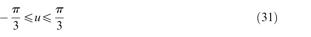
The steering angle is the key control input for the trajectory of the vehicle model. The only variable in the U vector is the steering angle. The constraints of the steering angle were set as follows:
Driving comfort: Lateral acceleration (
After correlating all vibration frequencies of the tests, the safe limit of acceleration for passenger comfort was determined be 0.38 g (3.73 m/s2). 26 Furthermore, it was suggested that passenger sickness was correlated significantly with low-frequency lateral accelerations. 27 The maximum lateral acceleration should be 1.3 m/s2 considering the design of highway and streets 28 ; however, in normal driving, a lateral acceleration ay ≤ 1.8 m/s2 is acceptable, 1.8 < ay < 3.6 m/s2 is tolerable, and ay ≥ 5 m/s2 exceeds the human’s tolerance. 29
To set a rational limit, the limit should be set with the tolerance of the simulation system error. The reference value is set to 0, and the constraints of lateral acceleration ±1.8 m/s2. The acceleration should be minimal in this study.

For wet and icy road surface. The lateral acceleration is constrained:

Driving smoothness: Driving is difficult.
30
A 5° steering requiring 3 s cannot be replaced by a 5°, 1.5 s steering since the vehicle will spinout. People tend to drive in a straight line. Drivers typically do not prefer a large steering rate as it deteriorates driving comfort. The rate of steering angle can be considered as an indicator of driving smoothness. As defined in the cost function in (23),

Intelligent trajectory: In some prior studies, the trajectory of AVs was overly conservative, which caused them to avoid every obstacle in an unhuman-centred way. Herein, an intelligent (human-centred) trajectory is introduced, in which within a drivable corridor, the ego vehicle can detect the speed of an obstacle. If the speed of the obstacle is 0, then it does not perform the full trajectory. Instead, it selects an optimal route within the drivable corridor.
In the intelligent trajectory, the lateral deviation from the reference safe route must be considered. The safe route is the line on which the minimum PF for all x-coordinates is located; however, it is irrational to drive along the safe route because the trajectory is conservative and can occasionally result in an overshoot in the lateral acceleration or a big yaw angle. Hence, a drivable corridor was established based on the safe route.
The distance of the lateral deviation was defined specifically. In a static obstacle scenario, the distance to the safe route can be larger (±1 m). In the dynamic scenario, the distance to the safe route based on the PF of the moving obstacle should be smaller (±0.5 m) since trajectory planning should be more conservative in a dynamic environment. According to the lateral deviation, a drivable corridor was established (see Figure 14).
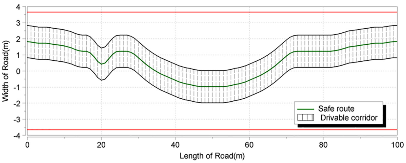
Drivable corridor of ego vehicle.
The deviation concept is illustrated in Figure 15. The lateral deviation can be calculated using (12) and (13). It was implemented in the simulation model.
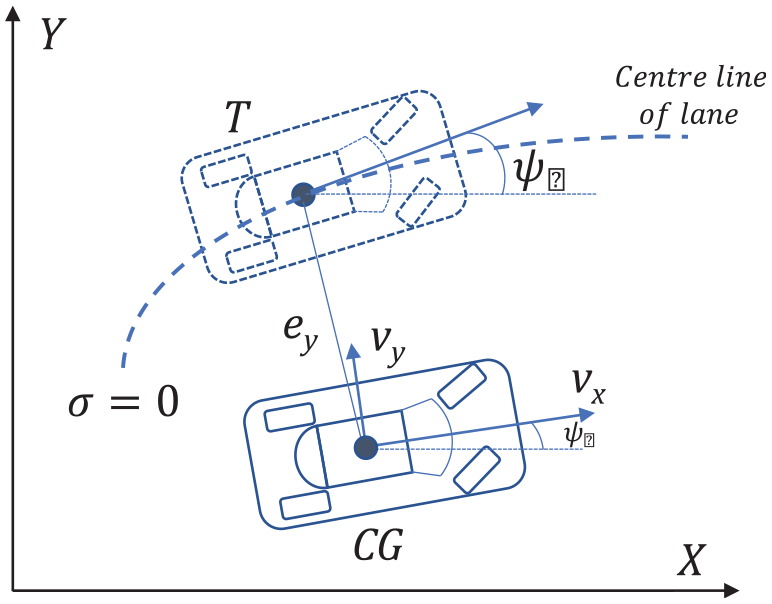
Vehicle’s deviation from safe route.
The variables of the MPC were set as shown in Table 2. The sample time was set to 0.1 s. The prediction horizon was 12; the control horizon was 2; the lateral position limits were −6 and 2 m from the edges of the road; and the starting lateral displacement was 0 in MATLAB.
Configuration of MPC.
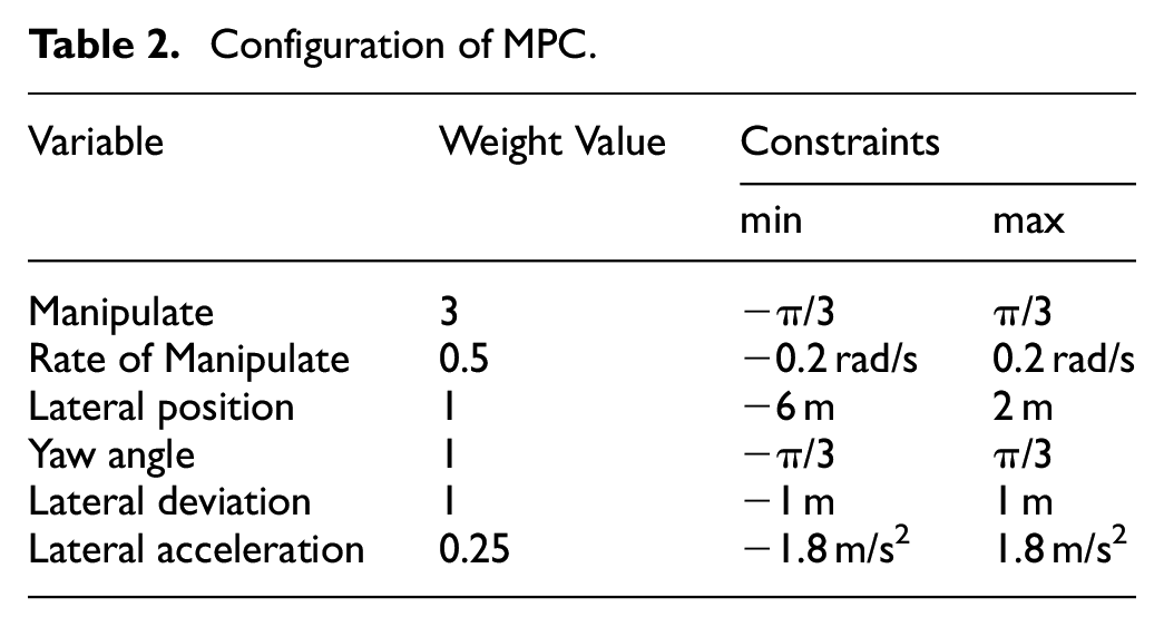
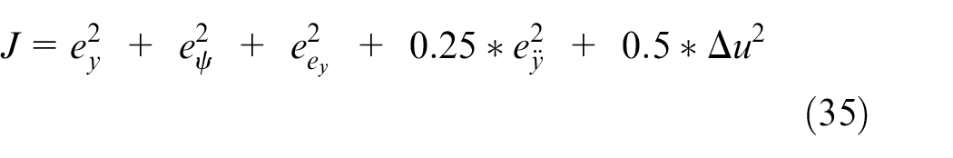
Based on (23) and the results of simulation tests, the variables of the MPC are listed in Table 2. The cost function used in this study was
The weight factors indicate that for trajectory planning in the static obstacle scenario, the control can be less conservative to allow for more lateral deviations. The driving comfort and smoothness are considered, but their weight factors are not as high as those for safety.
Simulation and analysis of results
Static obstacle avoidance
In the static obstacle scenario, the following simulation environments were established: the ego vehicle began its trajectory from (0, 0.825), (0, 1.825), and (0, 2.825). One nonmoving pedestrian was standing at (20, 3.65), and one nonmoving vehicle was situated at (50, 3.65). The vehicle measured 4 m × 1.5 m. Both sides of the road were covered with grass (see Figure 16).
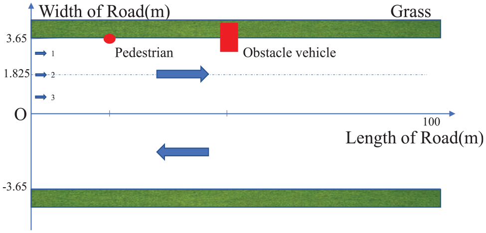
Traffic simulation environment in a coordinate system.
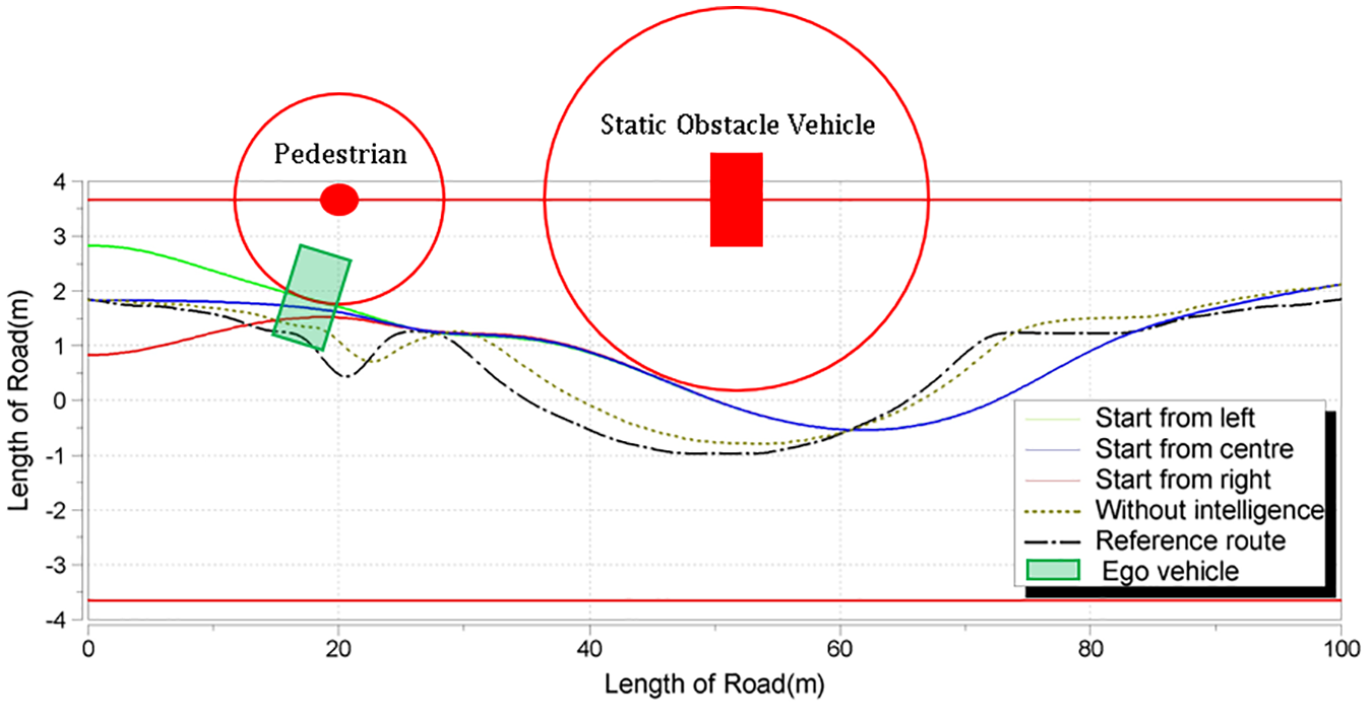
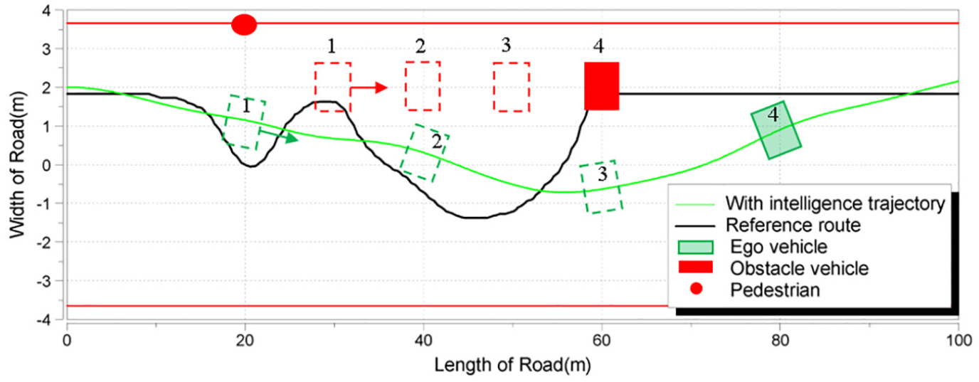
The driving scenarios are shown in the following figures. A comparison of all the simulation results with the safe route and the path-following control method (‘without intelligence’ in the figures) is shown (see Figure 17). The olive-colour curves in these figures represent the simulation results obtained using the path-following control method, which only follows the reference safe route; the black curve is the safe route with the minimum PF. The red straight lines indicate the edges of the road.
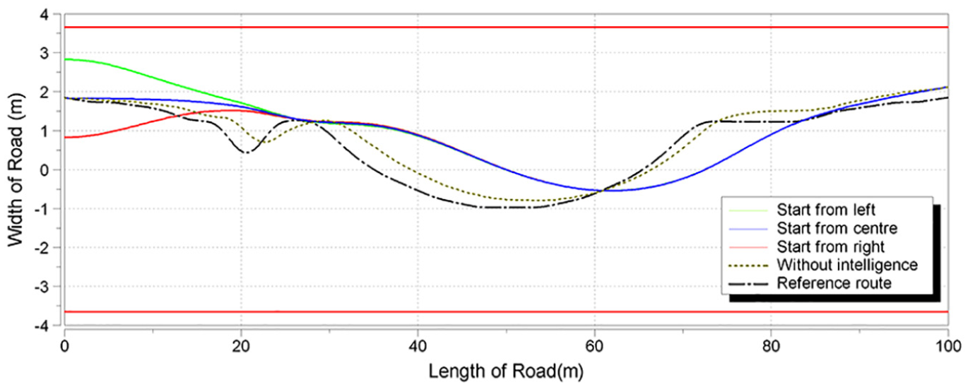
Comparison of the intelligent trajectory and safe route of simulation model.
The trajectory of the ego vehicle was similar to that of the intelligent MPC controller after 20 m (see Figure 17). They all drove in a straight line instead of in a curved route at the pedestrian location (x = 20), which required a large steering angle and resulted in a large lateral acceleration (see Figure 18). The trajectory did not follow the safe route at the obstacle vehicle (x = 50) since the safe route required a dynamic steering angle. The safe route returned to the centre line (x = 70), which again required a large steering angle change that was larger than 0.2 rad/s; this resulted in large lateral acceleration vibrations. The original safe route was overly conservative in that every obstacle was avoided, which is seldom observed in actual driving conditions. Therefore, the intelligent trajectory calculated by the MPC controller was human centred.
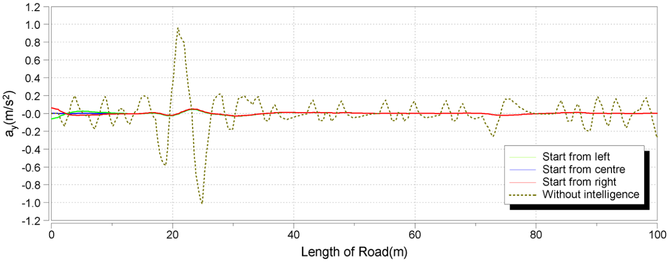
Comparison of the lateral accelerations.
The lateral acceleration difference between the intelligent trajectory and the other trajectories was significant. The lateral acceleration of the vehicle with a human-centred trajectory plan was within ±0.2 m/s2 (see Figure 18), which is not visible. 33 Meanwhile, the acceleration of the ‘path-following’ model contained a large vibration. The ‘jerk’ (derivative of lateral acceleration) of the models were also compared (see Figure 19); the jerk of the non-intelligent (without MPC) system was larger than the limit of 1.2 m/s3. 28
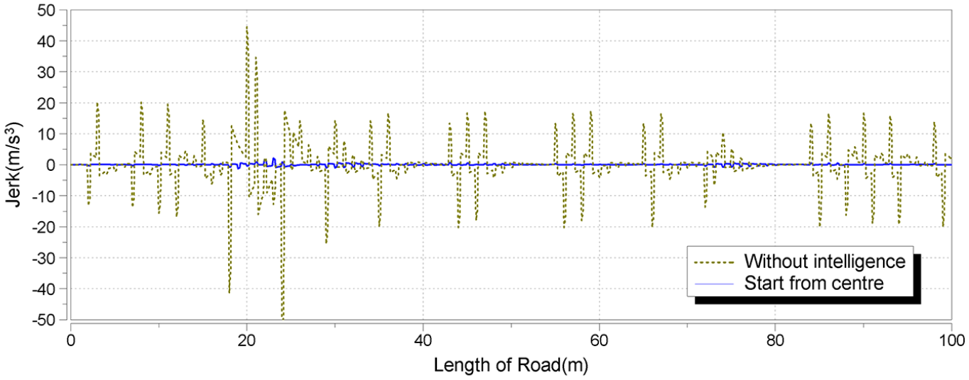
Jerk of models with and without intelligent trajectory plan.
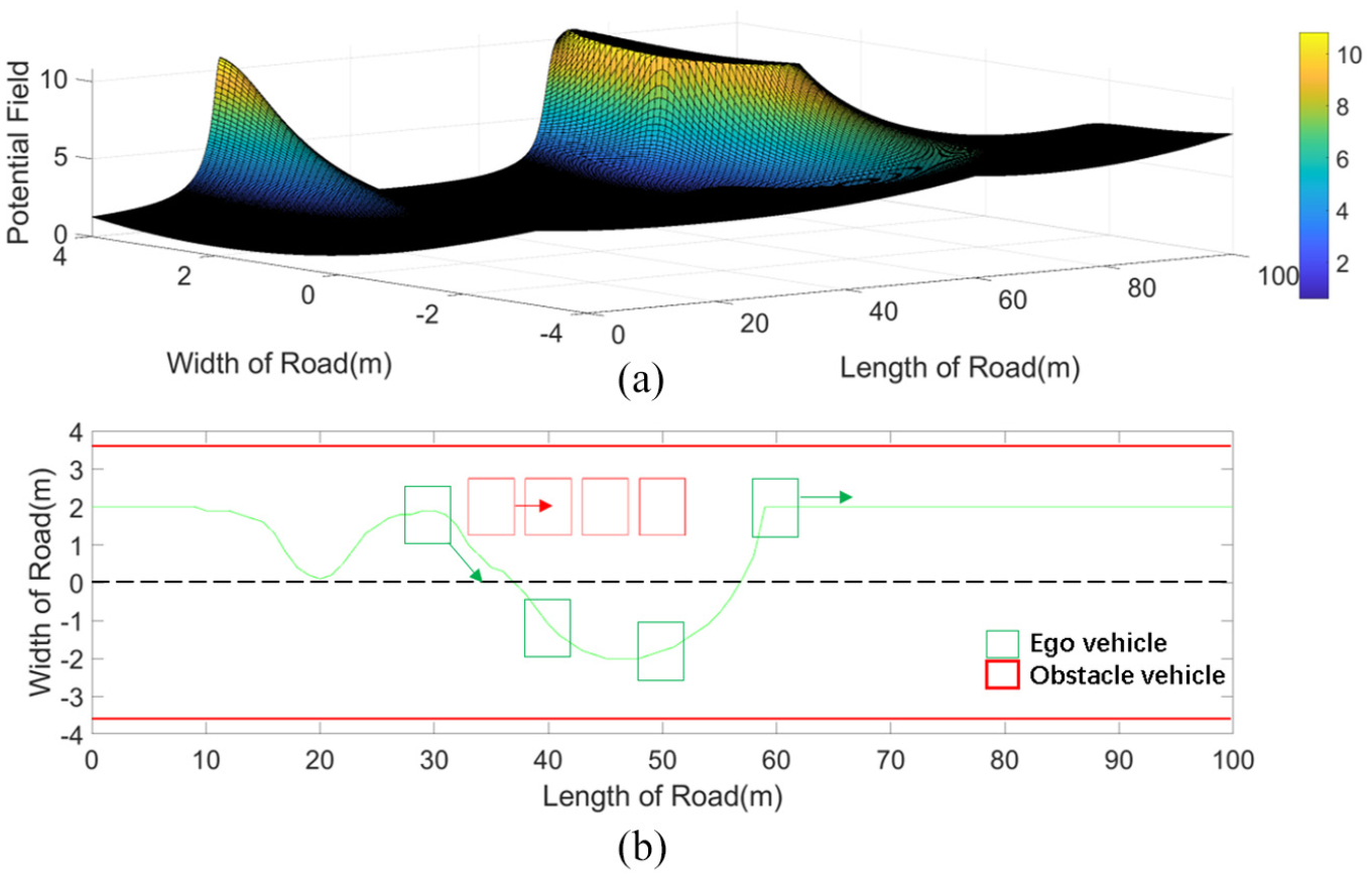
PF map and safe route: (a) 3D PF map and (b) ego vehicle’s safe route, ego vehicle positions(green), and obstacle positions (red).
The steering angle of the non-intelligent model varied between −0.50 and 0.73 rad (see Figure 21). The steering angle starting from the centre line was between −0.044 and 0.0467 rad, whereas that of the intelligent MPC model was smaller and smoother. The steering rate of the non-intelligent model was outside the limit of ±0.2 rad/s, whereas the steering rate of the intelligent MPC controller (blue) was within the limits (see Figure 22).
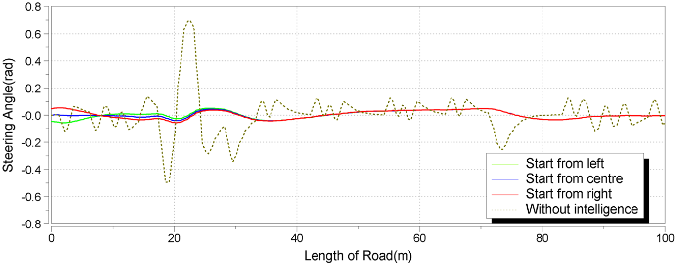
Comparison of steering angles.
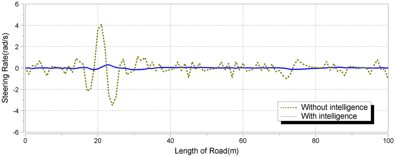
Steering rate of models with and without intelligent trajectory plan.
The distance from the ego vehicle to the static obstacle was calculated. The smallest distance between the pedestrian and the ego vehicle was 1.84 m. The minimum distance between the obstacle vehicles was 2.15 m (see Figure 23).
Distance between trajectory plan and obstacles in static obstacle scenario.
Dynamic obstacle avoidance
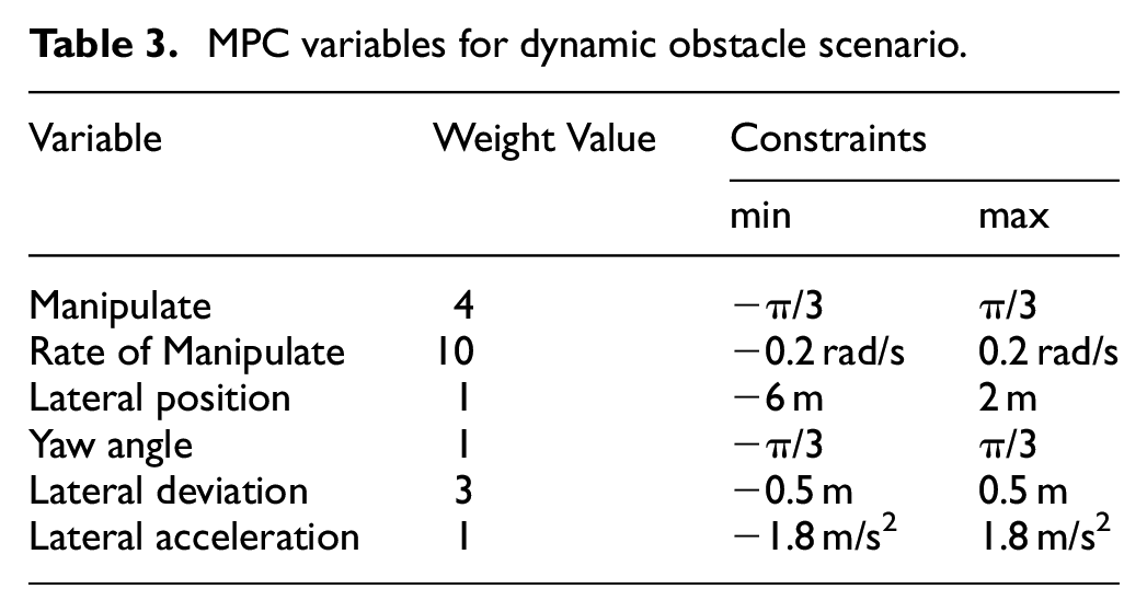
In this study, the dynamic obstacle avoidance scenario was set as follows: the nonmoving pedestrian was at (20, 3.65); the moving obstacle vehicle was moving from (20, 1.825) in the ego vehicle’s driving lane at a speed of 5 m/s; and the ego vehicle began moving from (0, 1.825) at the speed of 10 m/s. A safe route for the ego vehicle can be generated See Figure 20. Using the parameters in Table 3 to establish the MPC, the route of the ego vehicle can be calculated in the simulation. The optimised trajectory plan is shown in Figure 24.
MPC variables for dynamic obstacle scenario.
Trajectory plan and vehicle position in every 2 s.
Compared with the cost function of the static obstacle scenario, the dynamic scenario cost function focuses more on path following; accordingly, a larger weight factor is assigned to driving smoothness as the path following in a dynamic scenario may result in an abrupt steering.
The dashed-line rectangles represent the historical positions of the obstacle vehicle (red) and ego vehicle (green) (see Figure 24). The locations of the vehicles every 2 s are shown. The minimum distance between the COG of the obstacle vehicle and the trajectory plan was 2.74 m, which is at position 2 in Figure 24. The minimum distance between the vehicles was 1.23 m. The trajectory plan of the ego vehicle in the traffic scenario with a moving (1.5 m/s) pedestrian and that of the moving vehicle are shown in Figure 25.
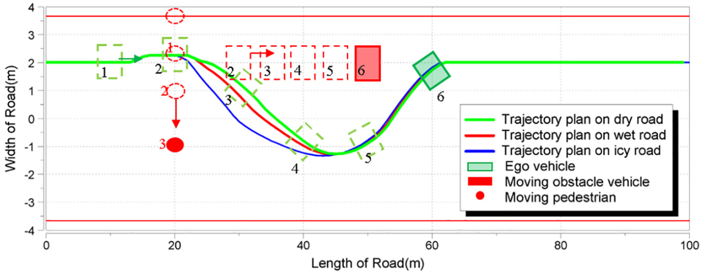
Trajectory plan with a moving pedestrian and a moving vehicle obstacle.
To validate the trajectory planning algorithm, the performance in the same scenario on wet and icy road is simulated. For the extreme road situation, potential field of obstacles are modified according to the adhesion coefficient (
Adaptive MPC obstacle avoidance
Using the adaptive MPC, human-centred trajectory planning can be implemented at different speeds (see Figure 26). As there are more factors involving in the adaptive MPC system and the system is more robust than the normal MPC, the trajectory planning difference between the intelligent and non-intelligent setups is small.
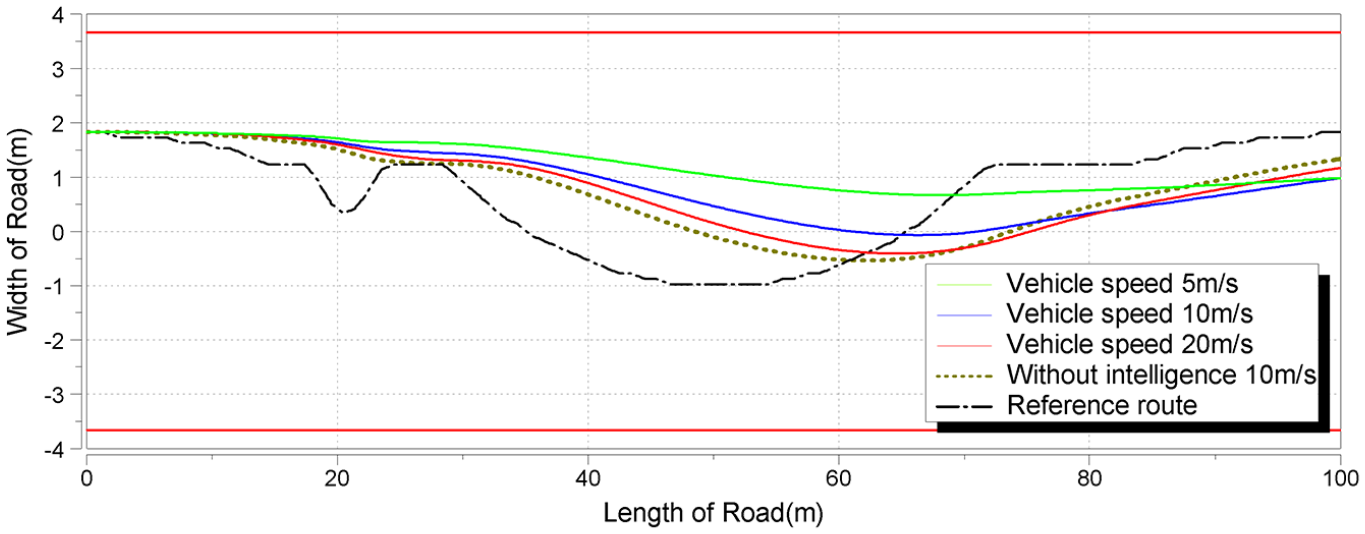
Trajectory plan of adaptive MPC at speeds of 5, 10, and 20 m/s.
The lateral acceleration with an intelligent MPC setup was one time smaller than the other model without intelligence (see Figure 27); however, both controllers exhibited small lateral accelerations.
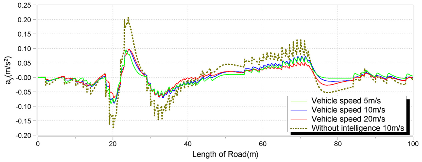
Lateral acceleration of adaptive MPC model at speed of 5, 10, and 20 m/s.
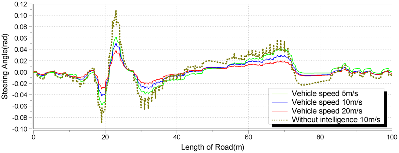
The steering angle of the adaptive MPC model at the speed of 5, 10, and 20 m/s.
The steering rate of the non-intelligent model was over the limit of 0.2 rad/s (see Figures 28 & 29), indicating that the trajectory was neither comfortable nor smooth.
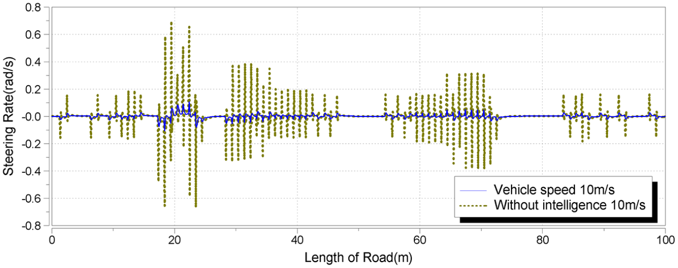
Steering rate of adaptive MPC model at speed of 10 m/s, with and without human-centred trajectory plan.
Conclusion
In this study, a human-centred trajectory planning algorithm was developed and tested in a simulation traffic environment. The planning method combines the PF algorithm with MPC real-time optimisation such that the potential risk level of the traffic environment can be evaluated efficiently, and a reasonable trajectory planning can be established. Using the PF algorithm, the risk to pedestrians, other road users and infrastructures could be evaluated; moreover, different static and dynamic obstacles were treated differently. Critical road surface situations were also considered. Different parameters were used in the MPC for static and dynamic obstacles to prevent the ego vehicle from being overly conservative or simplistic. Parameters of the PF and MPC were allocated based on literature review and tests performed. Scenarios with static and dynamic obstacles were investigated. The results demonstrated that the trajectory planning algorithm could perform well under dynamic scenarios. The ego vehicle was driven from different initial locations, and the trajectories demonstrated the robustness of the control, that is, the drive was completed reasonably and comfortably. Furthermore, control methods with and without MPC were investigated, the results of which demonstrated that the human-centred risk potential-based trajectory plan was smoother and more comfortable than the non-MPC method. The distance between the ego vehicle and obstacles under MPC was calculated, and the result indicated that safety was ensured.
In this study, it was assumed that the computer vision system was accurate; however, errors may occur in reality. Hence, an environment conception system must be implemented. To implement the proposed method in the real world, its online computational capacity must be evaluated. Critical road situations, such as icy and wet road surface were also be considered to assess the control algorithm, however, this topic should be discussed further. These will be endeavoured by the authors in future studies.
Footnotes
Appendix I
Author contributions
Zezhong Wang and Chongfeng Wei designed and carried out the research methods. Zezhong Wang and Chongfeng Wei carried out the simulation and analysed the results. Zezhong Wang and Chongfeng Wei discussed the results. Zezhong Wang wrote the manuscript.
Declaration of conflicting interests
The author(s) declared no potential conflicts of interest with respect to the research, authorship, and/or publication of this article.
Funding
The author(s) disclosed receipt of the following financial support for the research, authorship, and/or publication of this article: This study is partially supported by Sichuan Provincial Key Laboratory of Vehicle Measurement, Control and Safety (QCCK2020-001).