The prediction of measurement variability in an automotive application by the use of a coherence formulation

Abstract

Variability between nominally identical vehicles is an ever-present problem in automotive vehicle design. In this paper, it is shown that it is possible to quantify and, therefore, separate the measurement variability arising from a number of tests on an individual vehicle from the vehicle-to-vehicle variability arising from the manufacturing process with a series of controlled experiments. In this paper, coherence data is used to identify the measurement variability and, thus, to separate these two variability sources. In order to illustrate the methodology, a range of nominally identical automotive vehicles have been tested for NVH (noise, vibration and harshness) variability by exciting the engine mount with an impact hammer and measuring the excitation force and corresponding velocity responses at different points on the vehicle. Normalised standard deviations were calculated for the transfer mobility data, giving variability values of 25.3%, 33.5% and 37.3% for the responses taken at the suspension strut, upper A-pillar and B-pillar, respectively. The measurement variability was determined by taking repeat measurements on a single vehicle, and was found to be 2.9%. The measurement variability predicted by the coherence data on the multi-vehicle tests was compared with the directly taken repeat measurements taken on a single vehicle and these were shown to agree well with one another over the frequency range of interest.

Introduction

The levels of noise and vibration within a vehicle passenger cabin are often perceived as levels of quality by customers.^1,2 This is particularly true in the premium car market and is therefore of high importance. When determining benchmarks for vehicle design, some variability is to be expected in the vibration frequency response functions. This variability occurs not only in older vehicles from wear and tear but also in new components and in their assembled products due to manufacturing tolerances, assembly differences and environmental changes.

Studies^3–8 seeking to quantify the variability of the transfer mobility in automotive vehicles tend to find a 10–15 dB range. Due to the complexity of modern vehicles, with significant trim mass, stiffening reinforcements and the addition of controls and motors, the task of identifying variability sources is large, and it is for this reason that any external influences coming from the environment or measurement taking process should be properly quantified.

The frequency response function (FRF) can be defined as the ratio of the output spectrum $S_y\left(\omega \right)$ to the input spectrum $S_x\left(\omega \right)$ (which minimises noise at the output). The following definition will be used throughout this paper

$$H_{\mathrm{xy}}\left(\omega \right)=\frac{G_{\mathrm{xy}}\left(\omega \right)}{G_{\mathrm{xx}}\left(\omega \right)}=\frac{S_x\left(\omega \right){S^{*}}_y\left(\omega \right)}{S_x\left(\omega \right){S^{*}}_x\left(\omega \right)}$$

(1)

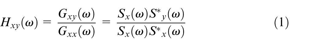
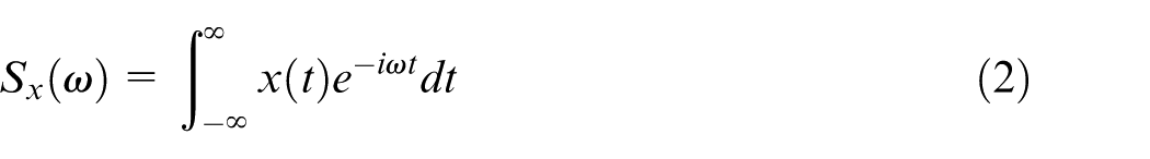
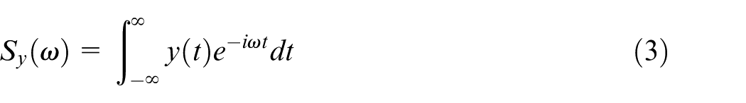
Where the subscripts x and y are the input and output signals respectively, ω is the angular frequency and $H_{\mathrm{xy}}\left(\omega \right)$ is the estimated FRF. The input auto power spectrum is denoted as $G_{\mathrm{xx}}\left(\omega \right)$ , and the cross power spectrum between the input and output is denoted as $G_{\mathrm{xy}}\left(\omega \right)$ .

The linear spectra $S_x\left(\omega \right)$ and $S_y\left(\omega \right)$ are found by taking the Fourier transform of the time domain signals as shown below where the continuous time t ranges between ∞ and -∞

$$S_x\left(\omega \right)={\int }_{-\infty }^{\infty }x\left(t\right)e^{-i\omega t}\mathrm{dt}$$

(2)

$$S_y\left(\omega \right)={\int }_{-\infty }^{\infty }y\left(t\right)e^{-i\omega t}\mathrm{dt}$$

(3)

Any result taken from a measurement of a random process is only an estimation of the true ensemble value, where the responsible factors that contribute to the uncertainty can range from the quality of the experiment to the ability of the operator taking the measurements. Thus, determining the level of a design of experiments is an important aspect that ensures the results are an accurate reflection of reality. Repeating the measurement a number of times under controlled conditions is a common method of reducing errors, while more rigorous methodologies, such as a design of experiments, ⁹ can be valuable tools in reducing and quantifying the uncertainty in measurements. A properly applied a design of experiments will isolate the individual variables that affect the measurement and determine the relative uncertainty of the influencing factors. If the standard deviation is lowered, thereby reducing the variability, fewer test samples will be needed. ¹⁰

Several studies give practical suggestions for reducing variability, such as keeping all accelerometers attached throughout the testing in order to eliminate any frequency shift that could arise from small changes in the measurement locations and to keep a low input force in order to prevent nonlinear behaviour. ¹¹ Design of experiments is part of a wider methodology ¹² created in order to be used at the design and manufacture stages of a product.

A hierarchical approach can also be useful as it distinguishes clearly between inter-variability, intra-variability and measurement uncertainty. Intra-variability is defined as the phenomenon leading to variation within a system as a result of changes in environmental conditions. Inter-variability is caused by manufacturing processes and the occurrence of component tolerances, leading to intrinsic variability in systems that would otherwise be nominally identical. ¹³ Overall variability is defined as a combination of these two types of variability as well as measurement variability.

It is the aim of the investigation reported in this paper to illustrate a novel method for predicting measurement variability. This will lead to a separation of the measurement variability from the vehicle-to-vehicle variability. Several investigations^3–8 into the variability of structure borne frequency response functions suggest that the cabin panels and coupling attachments between interfaces are components of high sensitivity that contribute significantly to the variability of FRFs. However, little is said on the variability that arises as a result of the measurement taking process and how external influences are controlled in order to ensure that different measurements are broadly comparable. Kompella and Bernhard’s investigation ⁷ does take structure borne FRF measurements on a reference vehicle; however, the structure borne normalised standard deviation of the magnitude is shown to vary by more than 100% for much of the frequency range. Tests used a loudspeaker as the excitation source and have previously shown that the structure borne FRF variability due to measurement techniques had, at worst, a value of ±2 dB, although on average the measurements varied by $\pm 1$ dB. ⁸

This study includes the testing of 16 nominally identical Range Rover Evoque vehicles to determine both the vehicle-to-vehicle variability and the measurement error. Section 2 gives the theoretical background into the error analysis that is applied to the measured data. Section 3 outlines the measurement method and in Section 4, an equation that links the experimentally measured coherence data to the normalised standard deviation (NSD) at the measured FRF data is applied in order to separate the measurement variability from the vehicle-to-vehicle variability. Section 5 draws conclusions from the analysis.

Error analysis and uncertainty prediction

Due to their complexity, a great many areas in engineering can show apparent stochastic behaviour. For example, where each measurement with a certain time history cannot be exactly repeated, it is necessary to collect a set of statistical data in order to describe the random process under study.

There are two main types of measurement error,^14,15 with the first being random errors, and the second being bias errors. Random errors can arise as result of noise in the system and to analyse the measurement, averaging functions may need to be applied. The second type of error often has the same magnitude across the frequency spectrum. For example, this can arise as a result of applying windowing functions or other digital signal processes.

The random error in a set of measured FRFs can be quantified by calculating the standard deviation and is determined by

$$s\left(f\right)={\left(\frac{1}{n-1}\sum _{i=1}^n{(\left|H_{\mathrm{xyi}}\left(f\right)\right|-\left|\overline{H_{\mathrm{xy}}\left(f\right)}\right|)}^2\right)}^{\frac{1}{2}}$$

(4)

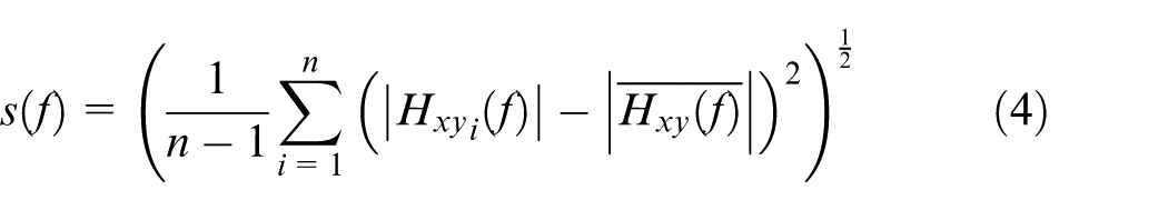
where s is the standard deviation, f is the frequency, n is the number of measurements, $H_{\mathrm{xy}}\left(f\right)$ is the FRF, the index i indicates the ith FRF and $\overline{H_{\mathrm{xy}}}\left(f\right)$ is the mean of the FRF at a specific frequency obtained by

$$\overline{H_{\mathrm{xy}}}\left(f\right)=\frac{1}{n}\sum _{i=1}^n|H_{\mathrm{xyi}}\left(f\right)|$$

(5)

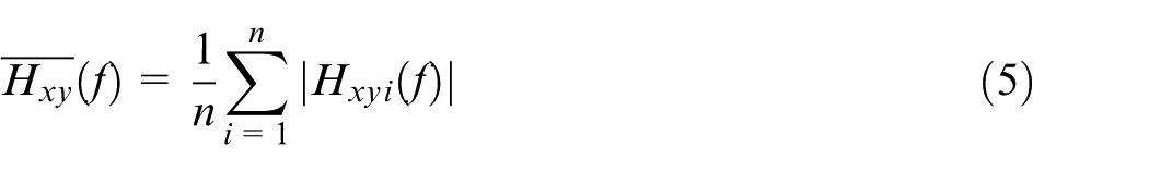
It is also convenient to represent the standard deviation as a fraction of the mean of the measured data. This allows different parts of the vehicle to be compared to one another. The NSD as shown in equation (6) uses the FRF’s mean to normalise the standard deviation and is known as the coefficient of variation or the NSD

$$\hat{s}\left(f\right)=\frac{s\left(f\right)}{\overline{\left|\overline{H_{\mathrm{xy}}}\left(f\right)\right|}}$$

(6)

As part of a wider study on statistical errors and coherence function measurement, an approximation developed by Bendat ¹⁵ provides a method of predicting the NSD from coherence data without the use of FRFs directly. Instead, the only inputs into the equation are coherence data, $\gamma$ ; var is the variance

$$\hat{s}\left(f\right)=\frac{\mathrm{var}{\left(\left|\overline{H_{\mathrm{xy}}}\left(f\right)\right|\right)}^{\frac{1}{2}}}{\overline{\left|\overline{H_{\mathrm{xy}}}\left(f\right)\right|}}\approx \frac{{(1-\gamma {\left(f\right)}^2)}^{1/2}}{\left|\gamma \left(f\right)\right|\sqrt{2n}}$$

(7)

It is assumed that the input signal is noise free (unlike the output) and that the noise and the input signal are incoherent. The use of equation (7) to effectively separate the measurement variability from the vehicle-to-vehicle variability is shown in the following section.

Measurement procedure

The point and transfer FRFs are obtained by using a calibrated accelerometer with a magnet attachment, an impact hammer and a high speed data acquisition system where the data is recorded and processed with commercial software, RT Pro Photon. In order to provide a test case and highlight the difference between measurement variability and vehicle-to-vehicle variability, measurements have been taken on a set of nominally identical Range Rover Evoque vehicles, all of which had five doors with the same engine variant and body structure (including panoramic roof). Any other small trim variations were assumed to be statistically insignificant.

A design of experiments was carried out prior to the measurement study, which investigated the output FRF variability as a function of temperature changes and the angle of incidence of the impact hammer. It was found that for small changes to the angle of incidence (90°± 20°), negligible variations were noticed when coherence was good (around a value of 1). At incident angles greater than 20° from a normal impact with the surface, a maximum variability of 10% can be expected by averaging the NSD over a 450–800 Hz frequency range. This variability source is reduced by taking averages over a set of repeat measurements.

The design of experiments and the literature showed that temperature can make a significant contribution to the intra-variability, ¹⁶ especially in the case of polymer materials. Thus, the tests were carried out within 30 min from start to finish, reducing any environmental effects of temperature changes which might yield different results for different materials in the vehicle. The collection of data was subject to time constraints, which meant that a total of 16 vehicles were tested. This compares to studies that were able to collect data from a greater number of vehicles.^3–5 However, this study differs in that a larger number of repeat measurements were taken for each individual vehicle. One study by Cafeo et al. ¹⁰ observed that by taking a large number of repetitions, an accurate set of data was obtained without the need for huge sample numbers. Their study took a sample of seven vehicles and tested each vehicle a total of nine times.

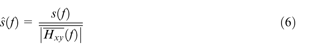
A total of 35 repeat measurements were taken at the top of the suspension strut and 19 measurements at the lower A-pillar (see Figure 1). These response positions were chosen as they are relatively stiff areas on the vehicle body, and previous large studies ³ have also used these same positions. The time and other practical constraints meant that the response positions needed to be easily accessible. A magnet was used to attach the accelerometers to the vehicle structure, which ensured good energy transfer to the accelerometers. The FRFs were recorded over a 0–1000 Hz range with the large time sampling duration of approximately one second with sampling intervals of 0.15 μs. The use of a metal-tipped impact hammer meant that the time intervals on the force profile occurred within a 0.1 ms time span, so it was necessary to have small enough sampling intervals to obtain a smooth impact profile. A set of FRFs was generated for each of the 16 vehicles using an average from five impacts. Each vehicle has five individual sets of FRF averaged readings which make up a spread of repeatable data.

Figure 1.

The three measurement response points where the accelerometers were placed. A more detailed image of the positioning of the accelerometer at site 1 can be seen in Figure 2a; this is obscured by the bonnet in Figure 1.

Multi-vehicle testing

Three locations on the vehicle exterior were chosen as measurement response points. Points two and three can be seen in Figure 1. These include the lower and upper A-pillar with the first measurement response site being a point near to the chosen hammer impact site. The third response point is at the suspension strut, located under the bonnet (Figure 2).

Figure 2(a).

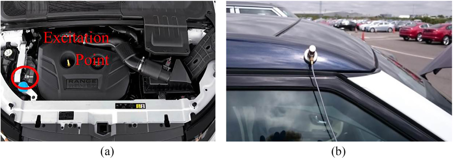
The photo shows the bonnet interior of a Range Rover Evoque, with the site at which the vehicle is excited with the impact hammer. (b) The measurement response position above the upper A-pillar. The accelerometers were held on with the use of a magnet.

Throughout the testing, checks for bad hits were carried out by observing the forcing input signal and the coherence. Any double hits that occurred were rejected, and the coherence was monitored to ensure that the data sets had a relatively high value (around 1). The use of a hammer excitation led to small differences in the sound produced with each impact. If the sound produced was unusual, the hit would be rejected.

Results and discussion

Measurement variability

In order to determine the measurement variability, repeat measurements of the FRF were taken from the engine mount to the suspension strut (35 times) and then from the engine mount to the lower A-pillar (19 times) on a single vehicle. An example of the transfer mobility determined from the response functions can be seen in Figure 3, where the different colours represent different sets of measurements made under the same conditions. The spread of the graph’s data is an indicator as to the variability of the repeated results and is an indicator of the NSD in Figure 4.

Figure 3.

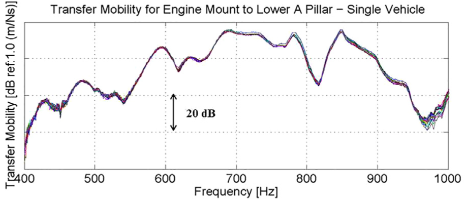
The modulus of the transfer mobility from the engine mount to the lower A-pillar was taken on a single car. The measurements have been repeated 35 times with each measurement shown in a different colour. The spread of the data represents the variability due the measurement taking process.

Figure 4.

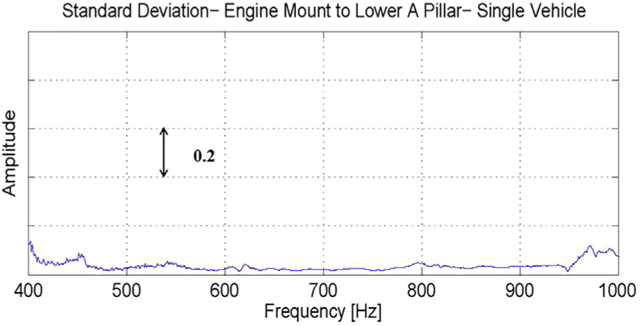
The NSD of the transfer mobility from the engine mount to the lower A-pillar for a single vehicle shown in the frequency range from 400 Hz to 1000 Hz.

Coherence can be used to determine the quality of the measured results. Figure 5 shows that the coherence data is good across the frequency range 450–800 Hz. The frequency range from 0 Hz to 450 Hz showed a poor coherence, which was due largely to the damping effect from engine NVH control solutions. The high damping levels on the vehicle meant that the transfer function measured mostly noise over this band. The overall measurement variability, therefore, is taken from 450 Hz to 800 Hz as in this range the coherence is found to have a value close to 1 (See Figure 5). In order to access the lower frequency characteristics with confidence in the results, the engine would have to be removed before the testing was done. However, this was not practical for the test vehicles available.

Figure 5.

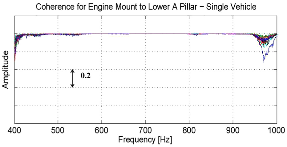
The coherence for the engine mount to the lower A-pillar. Each of the 35 colours represents the results of five repeat measurements.

The data was found to be highly repeatable over the frequency range, with NSD values of 2.5% and 2.9% for the engine mount to the suspension strut and engine mount to the lower A-pillar, respectively. The distance between the excitation point and the measurement response point also has an effect on the measurement variability. ¹⁷ Each time the signal passes through boundaries, such as hinges, rubber seals and welds, the variability in the measurement is found to increase. As the distance between the excitation point and response point increases, therefore, typically the measurement variability is also found to increase. This is reflected in the measurement variability results, which can be found in the vehicle-to-vehicle NSD results in the next section. These experimental results provide a benchmark for the measurement variability. In summary, good repeatability is seen for frequency bands that have coherence values around 1.

Vehicle-to-vehicle variability

Structural testing on the 16 nominally identical Range Rover Evoque models was carried out following the same method as described in Section 2. A sample of the transfer mobility data are shown in Figure 6. Each individual line plotted represents a single vehicle, and each result has been averaged over five individual hits. The coherence has been recorded in order to determine the data quality of the measurements, and the standard deviation calculations have also been included as a method in which the variability may be quantified. In order to identify and rank the variability of each set of measurements, a single value is calculated for each of the response positions. This is found by averaging the NSD data over a frequency range, which is determined by the coherence data in Figure 5. Thus, the NSD data within the frequency range of 450–800 Hz was found to vary by 25.3%, 33.5% and 37.3% for the suspension strut, the lower A-pillar and the upper A-pillar, respectively. Note that, as expected, the measurement variability increases with distance from the excitation point. These values are in a similar range, of 20–35% variability, when compared to other acoustic response variability studies. ¹⁸

Figure 6.

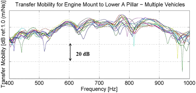
A comparison of transfer mobility graphs for the 16 nominally identical Range Rover Evoque vehicles tested with an impact hammer excitation from the engine mount and the response measured with an accelerometer above the lower A-pillar.

All three positions showed a large variability in the response data of each test. The difference between the single vehicle measurement and the vehicle-to-vehicle variability is shown more clearly in Figure 7, which gives the NSD of the position with the most variable FRF data (engine mount to upper A-pillar).

Figure 7.

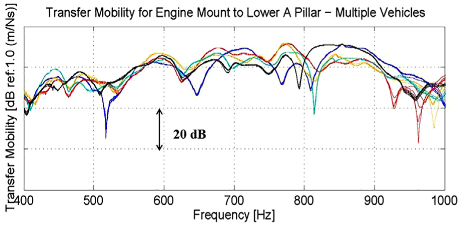
Transfer mobility data for a sample of five vehicles. Repeat measurements for each vehicle are shown in the same colour. Each colour represents the measured FRF of a single vehicle.

Figure 7 shows the results from five different vehicles taken at the upper A-pillar, each of which has several repeat measurements, which are shown in the same colour. It is possible to conclude that the measurement procedure had very little influence on the vehicle-to-vehicle variability.

Often when making experimental validations with finite element simulation results, only a single vehicle’s experimental data will be used. By observing the spread of results shown in Figure 7, it becomes clear that basing the expected performance of every manufactured vehicle on the simulated results of a single vehicle is likely to give unrealistic results due to the wide spread of experimental data. Even so, if uncertainty due to the measurement taking process could be predicted, then this information may be useful at the design stage by providing a spread of potential values at each frequency that may occur. The variation due to other sources such as manufacture, material tolerances and external influences would still have to be quantified, but could also provide uncertainty bands at the design stage.

Figure 8.

Comparison of the predicted with the measured NSD for the engine to lower A-pillar FRF data in the case of a single vehicle.

Implementation of the coherence function in order to predict the measurement variability

The ability to separate different variability sources with the use of a single formula provides a tool that can save time and money. The influence on the overall variability from the measurement process can be determined without having to carry out a separate single vehicle test. Figure 8 shows a comparison between the NSD data taken from a single vehicle and the predicted results after equation (7) has been applied to the coherence data. The two are found to be similar in amplitude across the frequency range, although slightly offset as the predicted data underestimates the actual variability. The difference between the directly recorded and predicted measurement variability could be reduced with the inclusion of a bias error. The prediction might also be improved by removing random noise at the input.

Figure 9.

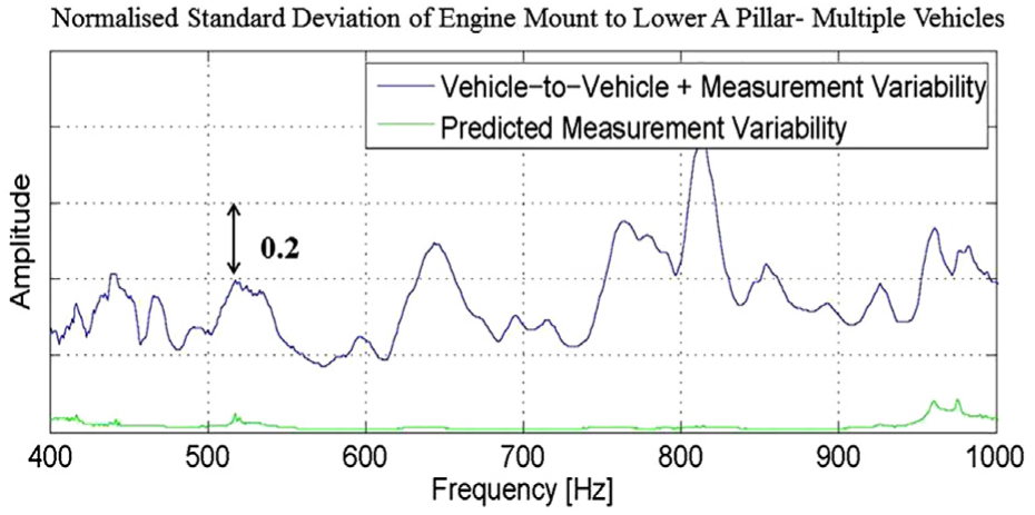
Comparison of the predicted with the measured NSD for the engine to lower A-pillar FRF data for all 16 vehicles.

The formulation, equation (7), is also applied to the vehicle-to-vehicle coherence data. The result of this can be seen in Figure 9, where the blue plot is the combined vehicle-to-vehicle and measurement variability recorded from the 16 nominally identical vehicles, and the blue plot shows the predicted measurement variability. Thus, by separating one set of data from the other, the separated measured variability data is given as shown in Figure 8.

Although the use of the coherence formulation can provide a good approximation to the measurement variability, it cannot provide any further information about the inter-variability. However, the estimation of the measurement variability provides a more realistic value of the inter-variability that can be applied to simulated results in the form of uncertainty bands.

Conclusions

Structural vibration FRF tests have been conducted on an ensemble of 16 Range Rover Evoque vehicles in order to determine both the vehicle-to-vehicle and the measurement variability. Three measurement response positions were tested: the suspension strut, the lower A-pillar and the upper A-pillar. An engine bracket mount was used as the excitation point. To obtain the measurement variability, a single vehicle was tested up to 35 times with an impact hammer and accelerometer. The NSD was calculated, and the measurement results were found to vary by up to 2.9%, which falls within the standard range seen in the literature. ⁵

The vehicle-to-vehicle variability was obtained by testing 16 nominally identical vehicles in the same manner. The NSD was calculated and produced values of 25.3%, 33.5% and 37.3% for the respective positions noted above. It was noticed that with increasing distance between the response at the accelerometer and the excitation location, the coherence would become increasingly worse. It is possible that this is due to the increasing number of components between the excitation and response points. Thus, it could be a result of the lack of signal energy from the impact hammer excitation reaching the accelerometer response.

The coherence data was used to predict the measurement uncertainty. By applying it without the need for extensive single vehicle tests, the measurement variability and the vehicle-to-vehicle variability can potentially be separated. The equation was validated on a sample of FRF data from a single vehicle. When the method was applied to the vehicle-to-vehicle variability data, the values were found to be very similar to the experimental measurement variability. The methods outlined here may be applied to other vehicles although the results shown are specific to the vehicles tested in this study.

Continued work to create an improved predictable measurement error will be carried out by taking into account the bias error for a multi-modal case. It would also be beneficial to include an FRF that minimises noise at the input. Using both types of FRF, noise would be minimised at both the input at output, however the two types of FRF form only a confidence interval for the true FRF rather than a single combined value. The results from this study could also be applied in a finite element context in the form of uncertainty bands on the predicted results.