
Abstract
For towering structures under complex time-varying excitation, the tuned magnetic fluid rolling-ball dampers (TMFRBD) cannot achieve self-tuning damping. In this paper, considering the operating characteristics of the TMFRBD, a damper self-tuning control algorithm, namely particle swarm optimization (PSO)-FUZZY-PID, is proposed for real-time adjustment of the intrinsic frequency of TMFRBD, which can greatly improve the damping effect, namely self-tuning magnetic fluid rolling-ball dampers (STMFRBD). Firstly, the equivalent dynamics model of the damping system is established, deriving the structural dynamic amplitude response as a function of the excitation frequency to structural frequency ratio. Different frequency tracking schemes of the damper are compared and analyzed. Then magnetic field simulations and magnetic fluid magnetic property measurements are performed for the dampers, respectively. Secondly, the self-tuning PSO-FUZZY-PID control algorithm is designed to improve the damping performance of STMFRBD under time-varying excitation by optimizing factors of the FUZZY-PID controller with PSO. To confirm the effectiveness of the damper self-tuning control algorithm, the frequency tracking of dampers with different control algorithms under time-varying excitation is compared. The results show that the damper’s frequency can be tuned quickly and accurately tracking excitation frequency by PSO-FUZZY-PID. Finally, the simulation and experimental results of STMFRBD and passive mass damper (PMD) under different loads are analyzed, and the structural amplitude response is analyzed using the Hilbert-Huang transform (HHT). In addition, the damping of STMFBD and TMFBD under different loads is compared. The results show that STMFRBD has better vibration-damping performance than PMD and TMFRBD.
Keywords
Introduction
Due to the high flexibility and low stiffness of the components in the higher horizontal position of the towering structures, 1 resulting in a structure that is susceptible to large oscillations caused by external vibrations, the vibration problem regarding the towering structure has received wide attention. 2 The current research on dampers for towering structures generally falls into three categories. The first type of passive dampers, 3 for instance, tuned mass dampers, 4 tuned rolling-ball dampers, 5 tuned liquid dampers. 6 This type of damper has a simple structure and does not consume external energy, but it cannot tune its operating state according to the complex excitation, which leads to a poor damping effect. The second type of active dampers, 7 for instance, using an acceleration negative feedback control algorithm to suppress structural vibration, 8 vibration suppression of towering structures using fuzzy sliding mode control, 9 and designing a novel neural network control strategy to suppress towering structural vibration. 10 These dampers can apply control forces to suppress vibrations under different excitations in a short period, but they require a large amount of external energy for operation. The third type of semi-active dampers is based on passive dampers and supplemented by active control means. 11 Therefore, this damper has the advantages of both and only requires less electrical energy to tune the damping performance. The current research on semi-active dampers focuses on smart materials, 12 for instance, magnetic fluid (MF), 13 magnetorheological fluid (MRF), 14 Since the smart materials can be adjusted according to external needs, they have a wide range of applications in damping, lubrication, etc.15,16 Due to the large yield stress and damping force of MRF, it has been widely used in the field of damping, for instance, MRF dampers with double annular damping gap, 17 Integral MRF dampers, 18 MRF dampers for FUZZY-PID controller. 19 However, micron-scale MRF tend to aggregate and precipitate with poor stability.
Unlike MRF, the nanoscale MF has higher stability and its unique magneto-viscous effect and zero hysteresis response under magnetic fields, which also has a simple vibration-damping structure and low response frequency.20,21 Magnetic Fluid (MF, also known as Magnetic Liquid or Ferrofluid), is a highly stable colloidal solution consisting of surfactants encapsulated with nanoscale magnetic particles and homogeneously dispersed in a base carrier fluid. 22 Abe et al. 23 conducted the first experimental study on the wobble characteristics of tuned MF dampers under a dynamic magnetic field and revealed the damping mechanism of the dampers. Kondo et al. 24 proposed a tuned MF column damper to suppress structural vibration over a wide frequency range. Oyamada et al. 25 designed tuned MF dampers using MF as the working fluid and changed the intrinsic frequency of the dampers by external coils. Ikari et al. 26 proposed a semi-active tuned MF column damper and studied its damping characteristics using two electromagnets. Ohno et al.27,28 designed a semi-active tuned MF damper and conducted a series of numerical simulations and experiments. Li et al. 29 proposed a new MF damper not only for structural damping but for energy conversion to improve damping efficiency. Previous studies have shown that the damper’s intrinsic frequency can change with the external magnetic field. However, in low-frequency operation, it is generally believed that only the upper MF of the damper is involved in the operation, while its lower MF is not involved in the operation, so it is not effective in damping low-frequency vibrations. To solve the problem that the MF in the damper does not fully participate in the work, Yang et al. 30 proposed a tuned MF rolling-ball damper (TMFRBD), effectively suppressing the towering structure’s low-frequency vibration by involving all MF in the operation.
Although TMFRBD can suppress the towering structural low-frequency vibration, when encountering complex time-varying excitation, the damper will be difficult to effectively attenuate the complex external vibration, because it cannot tune its parameters in real-time with the external excitation. Therefore, it is important to design a fast, accurate, and stable control algorithm to realize self-tuning damping. This paper considers the operating characteristics of the TMFRBD and proposes a damper self-tuning control algorithm, namely Particle Swarm Optimization (PSO)-FUZZY-PID, and factors of FUZZY-PID controller are optimally adjusted with PSO, to improve the damping performance of TMFRBD under time-varying excitation. The TMFRBD combined with the self-tuning control algorithm is defined as a self-tuning TMFRBD (STMFRBD). STMFRBD can track the change of excitation frequency to tune its intrinsic frequency in real-time to realize the tuned damping. In this paper, the damping system equivalent dynamics model is established, deriving the structural dynamic amplitude response as a function of the excitation frequency to structural frequency ratio, and comparing the changes in the amplification factor of STMFRBD under different frequency tracking schemes. Then a damper self-tuning control algorithm, namely PSO-FUZZY-PID, is designed to compare different control algorithms for the damper’s frequency tracking under time-varying excitation. And the damping performance of STMFRBD is verified by simulation and experiments, and finally, conclusions are given.
STMFRBD determination of frequency tracking scheme
Kinetic analysis of STMFRBD with the structure
Figure 1(a) shows the simulated towering structure using a single-degree-of-freedom frame. The STMFRBD consists of a rolling-ball, MF, a hemispherical recess, and an electromagnetic coil. Where the recess is rigidly connected to the top of the structure, the sum of the two masses is ms, and the structural damping and stiffness are c, k. The rolling-ball mass and radius placed in a groove with radius r1 are m1, r2, the ball contains MF with the mass of m2, and the ball drives the MF to roll along the hemispherical groove surface together. It is equating Figure 1(a) the single-degree-of-freedom frame with STMFRBD to the two-degree-of-freedom mass-spring-damping system in Figure 1(b). Where the vibration body equivalent damping, stiffness, and mass are c1, k1,
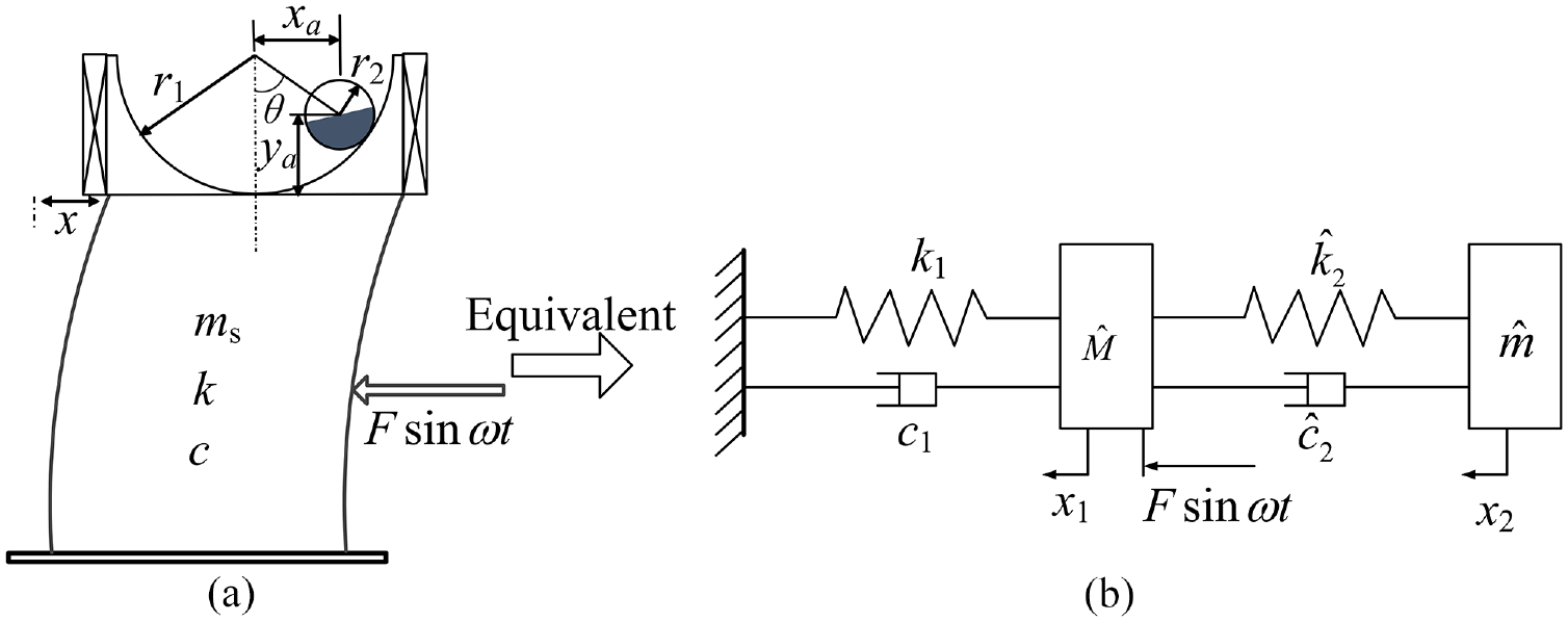
Equivalent model of damping system: (a) structure additional STMFRBD mechanical model and (b) two-degree-of-freedom mass-spring-damping system.
From Figure 1(a), the system kinetic energy T includes the vibrating body’s horizontal kinetic energy, the rolling-ball with the MF horizontal and vertical direction of translational kinetic energy, and the rolling-ball rotational kinetic energy:
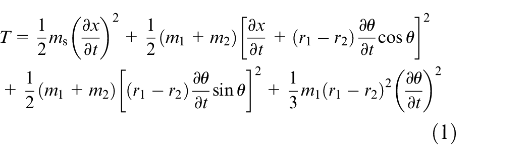
Where x is the structural top horizontal displacement, θ is the rolling-ball moving around the circular center of the groove angular displacement.
Assuming that the magnetic particle of MF is rotated by an angle Δθ under the magnetic torque

Since
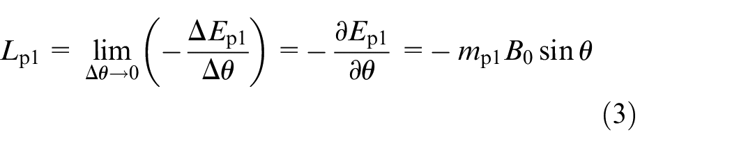
For magnetic particles suspended in an MF, in general

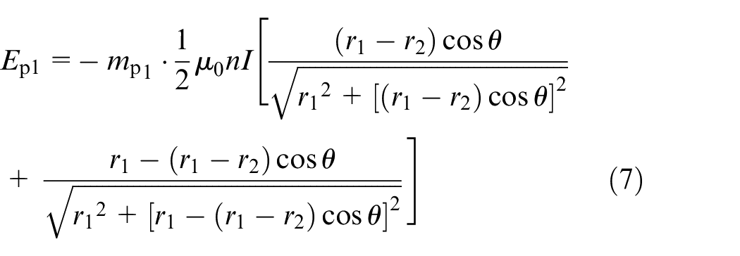
For TMFRBD, the internal magnetic field is generated by a cylindrical solenoid coil fed with DC current, and the magnetic field strength on the axis of the solenoid is:
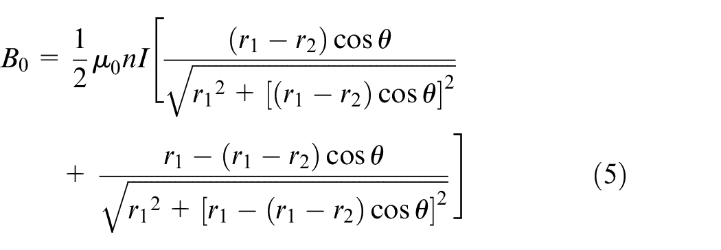
Where n is the turns of electromagnetic coil wound outside the groove, and I is the electric current.
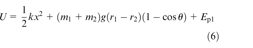
The system potential energy U consists of the elastic potential energy, the rolling-ball and the MF gravitational potential energy, and the magnetic particles potential energy, where the magnetic particle potential energy is combined with equations (4)–(5):
The Lagrange equation can be expressed as 31 :
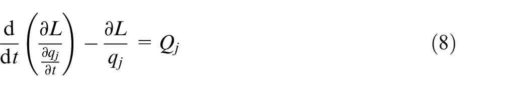
Where L = T-U, qj is the generalized coordinate, Qj is the generalized force, j is 1,2….
Assuming that the rolling-ball outer wall surface and the groove are smooth, the friction between the two can be ignored. For the system in Figure 1(a), the generalized coordinates are q1=x, q2=
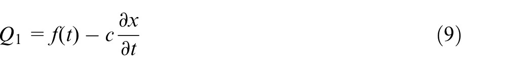
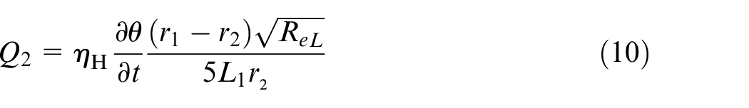
Where ReL is the Reynolds number, and ηH is the MF’s viscosity. Combining equation (1) and equations (6)–(10) and gives:
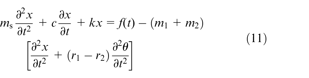
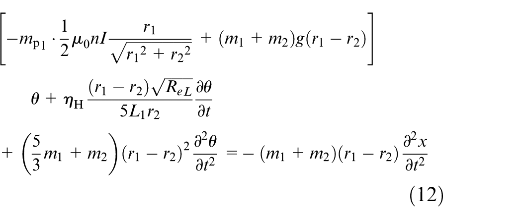
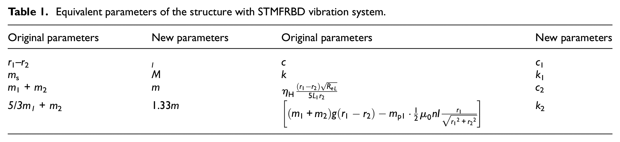
Where f(t) is externally applied force. From Figure 1(a), the horizontal and vertical displacements of the rolling-ball are xa(θ) = (r1−r2)sinθ, ya(θ) = r1−(r1−r2)cosθ. Since θ is relatively small, it can be approximated sin(θ) ≈θ, cos(θ) ≈ 1. At this time (r1−r2)θ is the rolling-ball horizontal displacement, and r2 is vertical direction displacement, that is, the vertical displacement can be ignored at this time. Since m1 is approximately equal to m2, therefore, when replacing m1 + m2 with m equivalent, it is easy to get 5/3m1 + m2 = 1.33m. Table 1 shows other equivalent replacement parameters for equations (11)–(12).
Equivalent parameters of the structure with STMFRBD vibration system.
Assume that xA is the rolling-ball relative to the ground displacement, x is the structural top relative to the ground displacement, then lθ = xA-x is the rolling-ball relative to the structural top displacement. Combine the parameters in Table 1, substituting this into equations (11)–(12), and organizing it yields:
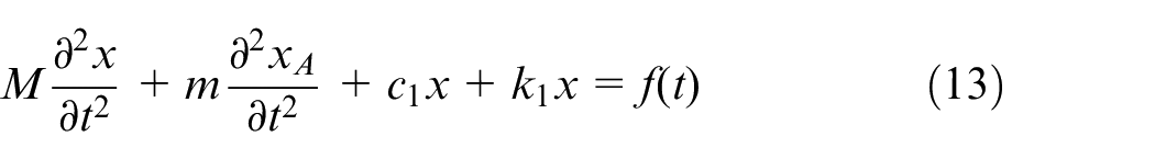
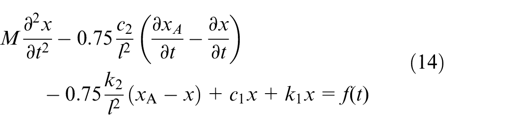
Make
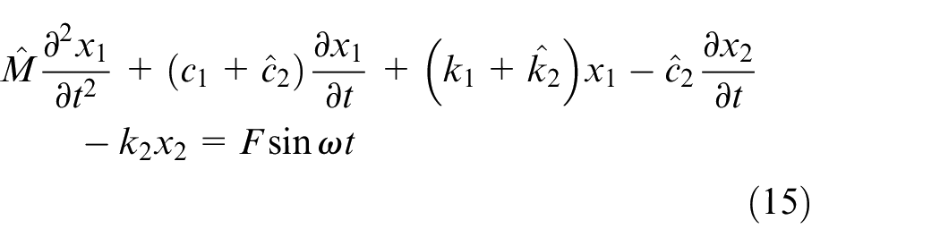
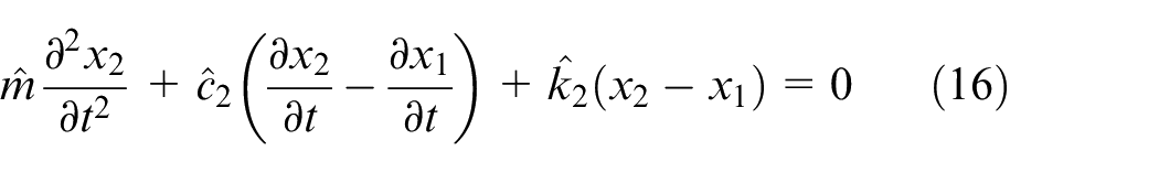
Equations (15)–(16) is the equivalent kinetic equation of Figure 1(b), then the displacement x1, x2, and the external excitation force F in the equation can be expressed in the complex form respectively
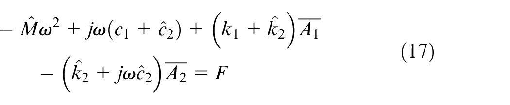
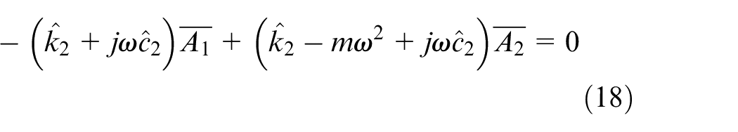
Combining with equations (17)–(18), the top amplitude of the structure can be:
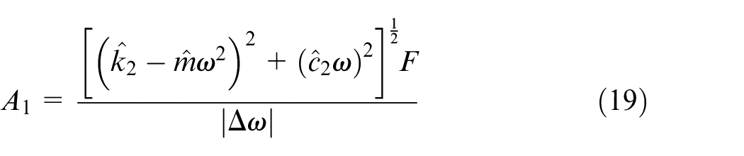
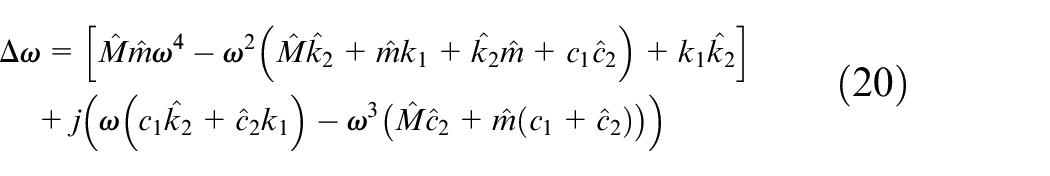
Assume that the structural intrinsic angular frequencies and STMFRBD are
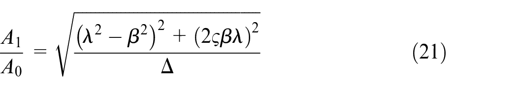
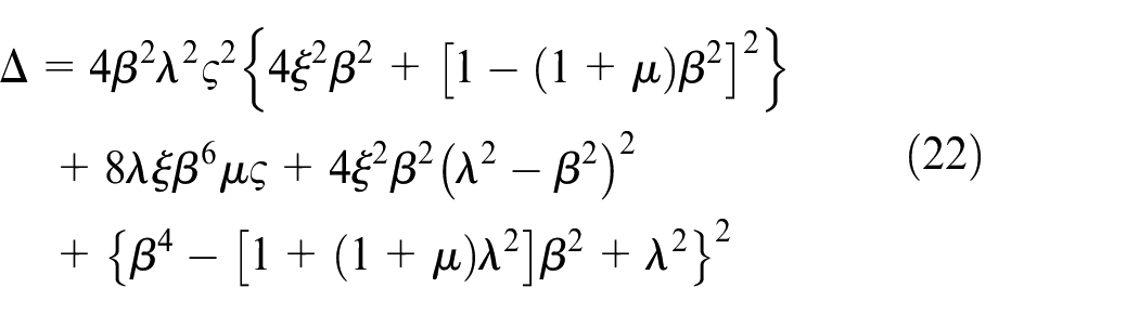
From equations (21) and (22), A1/A0 is related to the parameters λ, ς, β, μ,
Variation of amplification factor under different parameter schemes
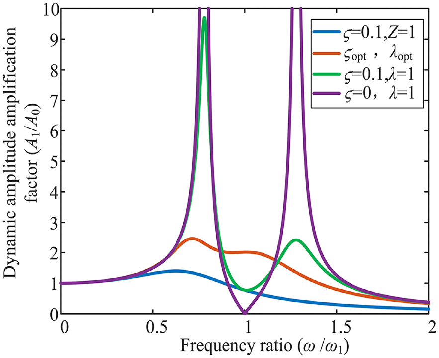
When μ,
Effect of different parameter ratios on the amplification factor.
As can be seen from Figure 2, when ς = 0.1 and λ = 1, A1/A0 becomes smaller compared to ς = 0 and λ = 1, indicating that a larger damping ratio can reduce the dynamic amplitude amplification factor. From the damping theory, it is known that the optimal damping ratio and frequency ratio expressions 32 :
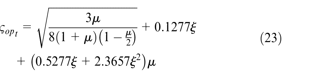
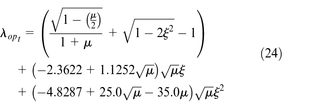
Combining equations (23) and (24), the red curve can be obtained as in Figure 2, which shows that a damper with optimal parameters can further reduce the amplification factor. The blue curve is ς = 0.1 and Z = 1, which means that the damper frequency changes with the excitation frequency. From Figure 2, the blue curve has the most minor amplification factor, which indicates that compared with the passive dampers without optimization and with optimal parameters, the frequency tracking scheme at Z = 1 has a good damping effect.
To confirm that Z = 1 is the optimal frequency tracking scheme, compare the other tracking schemes with the scheme when Z is 1. Let Z vary in the range of 1.0–1.5 and 1.0–0.5 to obtain the curves shown in Figure 3.

Effect of different tuning ratios on amplification factor: (a) Z = 1.0–1.5 and (b) Z = 0.5–1.0.
From Figure 3(a), the dynamic amplitude amplification factor increases and then decreases when the frequency ratio increases, and increases with Z. From Figure 3(b), the structural dynamic amplitude amplification factor increases as Z decreases. When ω/ω1 is less than 0.78, the amplification factor when Z is 1 is slightly higher than that when Z is less than 1. For Figure 3, when ω/ω1 is larger than 0.88 and Z is 1, the amplification factor decreases rapidly with the increase in frequency ratio. From the whole frequency ratio, when Z is 1, the amplification factor can be effectively reduced. Therefore, a frequency tracking scheme with Z = 1 can be used for the vibration of the structure during time-varying excitation.
Magnetic properties of MF and STMFRBD magnetic field simulation
In order to further analyze the performance of STMFRBD, this section measured the magnetic properties of the used kerosene-based MF (Base carrier fluid and surfactants account for 92% of the total volume of MF by volume, while solid-phase ferromagnetic particles account for 8%.), and the measurement results are shown in Figure 4, to analyze the main factors affecting the magnetic properties of the MF.
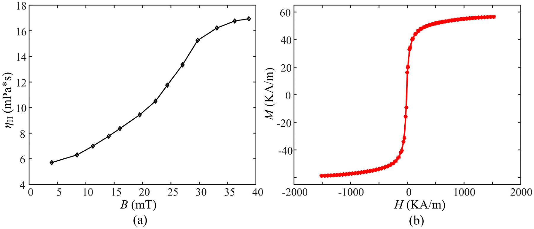
Magnetic properties of MF: (a) magnetic viscosity properties and (b) magnetization properties.
From Figure 4(a), the viscosity of the MF varies in the range of 5.8–17.6 mPa*s under the action of the magnetic field of 0–40 mT. From Figure 4(b), when the external magnetic field varies in the range of −500–500 kA/m, the MF is not saturated and the relationship between its magnetization strength and the excitation field is approximated as M = χmH, where χm is the magnetization rate of the MF. When the external magnetic field reaches about 500 kA/m, the MF reaches saturation.
Therefore, the viscosity and magnetization characteristics of the MF can be changed by an external magnetic field. When the applied magnetic field does not exceed the range that saturates the MF, the magnetic properties of the MF can be effectively changed, and thus the adjustment of the damper performance can be achieved.
To further investigate the magnetic field variation of the damper at different positions, the geometric model of the damper is first established, followed by the calculation of the magnetic field distribution inside the damper, and the established model and calculation results are shown in Figure 5.
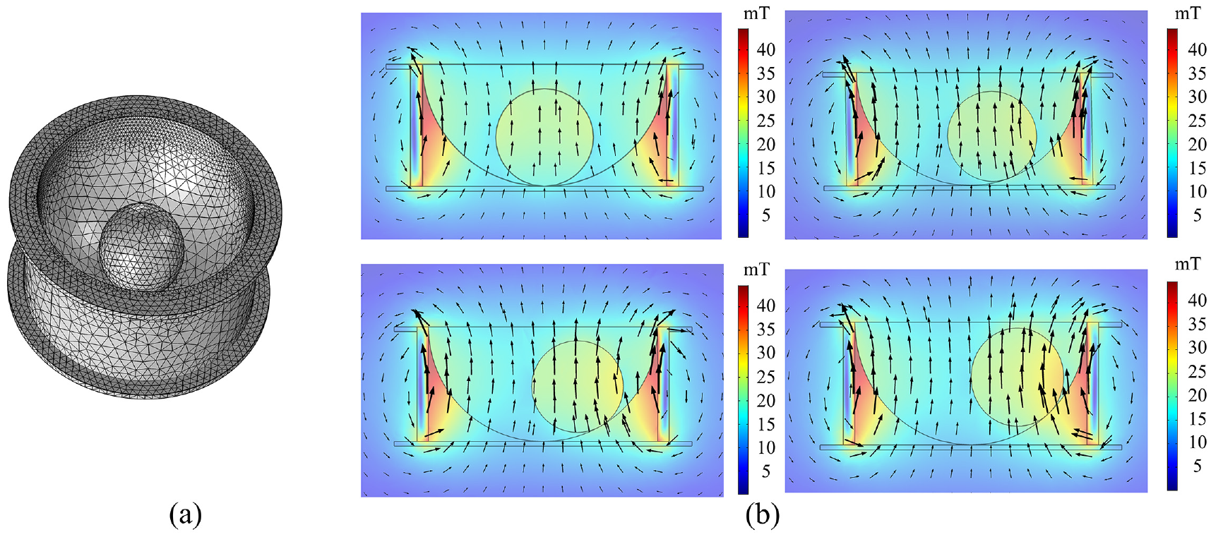
Simulation of the magnetic field of the damper: (a) model of the damper and (b) magnetic field distribution at different positions.
From Figure 5, the magnetic field distribution in the damper recess has good symmetry, and its magnetic field increases and then decreases along the central axis from bottom to top. Combined with Figure 4, the magnitude and direction of the magnetic field in the damper groove meet the requirements for adjusting the magnetic properties of the MF. Therefore, when the ball is in any position in the groove, the external magnetic field can effectively change the magnetic properties of the MF and then adjust the inherent frequency of the damper to achieve the purpose of tuning vibration reduction.
Damper self-tuning control algorithm design
The conventional FUZZY-PID controller can compensate for the PID deficiency to some extent. However, since its quantization and scaling factors are constant, it often fails to meet the required control performance for time-varying excitation. Considering the operating characteristics of TMFRBD, a damper self-tuning control algorithm, namely PSO-FUZZY-PID, is proposed, which can adjust the controller factor under time-varying excitation in real-time, and then tune the TMFRBD intrinsic frequency to track the main frequency of excitation in real-time. Figure 6 shows the damper self-tuning control algorithm principle.
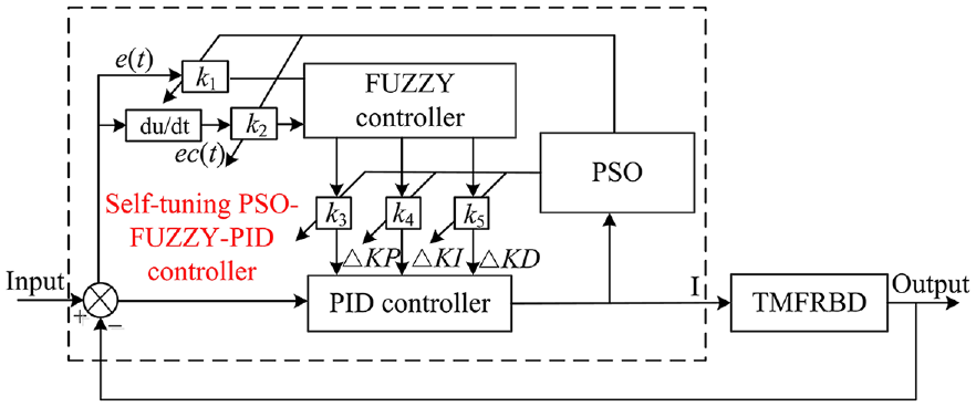
Damper self-tuning control algorithm schematic.
From Figure 6, it is clear that the damper self-tuning control algorithm contains the FUZZY controller, PID controller, PSO, quantization factors k1, k2, and scaling factors k3, k4, k5, etc. The FUZZY controller’s factors are rectified with PSO, where k1 and k2 maps the error and error change rate in the fundamental domain to the fuzzy controller input domain, and k3, k4, and k5 maps the fuzzy controller output to the output of the fundamental domain. For time-varying excitation, the intrinsic frequency of TMFRBD should be tuned in real-time to ensure the minimum response amplitude of the structure. The optimal factor during the time-varying excitation can be obtained by PSO, and then the optimal electric current of the FUZZY-PID controller output can be adjusted in real-time to tune the intrinsic frequency of TMFRBD in real-time.
FUZZY-PID control algorithm design
PID is a classical control algorithm, suitable for accurate mathematical models and linear systems. When the controlled system is nonlinear and has time-varying uncertainty, PID is no longer applicable. Fuzzy control is applied to nonlinear time-varying systems and is one of the most widely used intelligent algorithms, which can not only identify the error but also adjust the controller factors online according to its change trend. By combining fuzzy control with PID, self-tuning of PID parameters can be achieved. 33 The fuzzifier can be described as:

Where the input controller TMFRBD intrinsic frequency error and error change rates are E and EC, the TMFRBD intrinsic frequency error and error change rates are e(t) and ec(t). Positive big (PB), positive medium (PM), positive small (PS), zero (Z), negative small (NS), negative medium (NM), and negative big (NB) represent the seven fuzzy partitions into which E and EC are divided. According to the control law of TMFRBD intrinsic frequency tune, Table 2 displays fuzzy control rules.
Fuzzy control rule table.
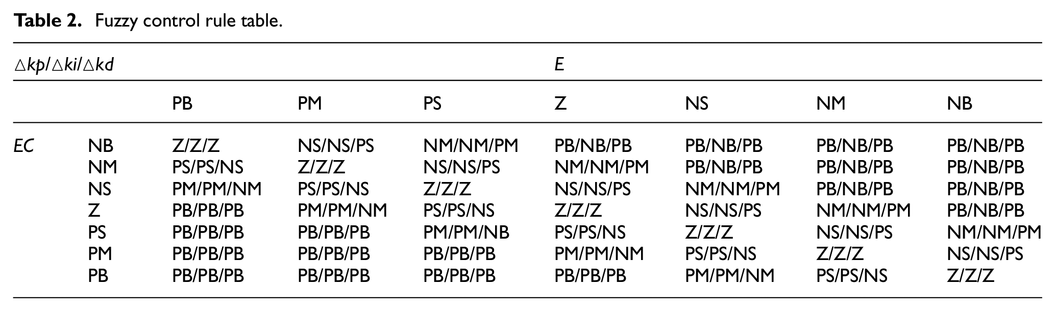
The FUZZY-PID controller involves five triangular affiliation functions and two gauss affiliation functions. The fuzzy rule surfaces of the affiliation functions for three parameters are shown in Figure 7, where E, EC, Δkp, Δki, and Δkd are [−0.1, 0.1]. The fuzzy inference of the controller is done by the Mamdani method.
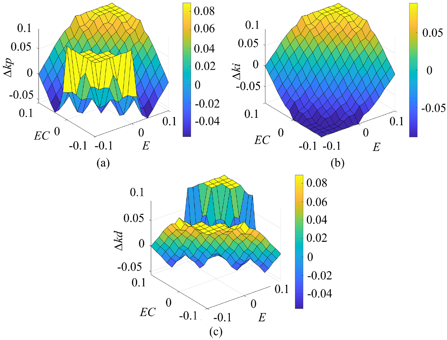
Fuzzy regular surface: (a) △kp, (b) △ki, and (c) △kd.
From Figure 7, the darker the yellow color indicates that the system output is a more positive value, and the darker the blue color indicates that the system output is more negative. The defuzzifier controller can be expressed as:

Where the controller outputs are Δkp, Δki, and Δkd, and k3, k4, and k5 are the scaling factors.
PSO-FUZZY-PID control algorithm design
Particle swarm optimization (PSO) is a bird flock activity swarm-inspired optimization algorithm. 34 The algorithm first generates a set of random solutions and iterates continuously to find the optimal solution. The FUZZY controller’s factors in this paper are optimized in real-time with PSO, which can achieve the maximum amplitude attenuation of the dampers to the structure under time-varying excitation.
Assume that the positions and velocities of the N particles composing a cluster are used to represent a D-dimensional vector, namely xij=(xi1, xi2, xiD), vij=(vi1, vi2, viD). The particle velocity and position are updated iteratively by the following equation 35 :

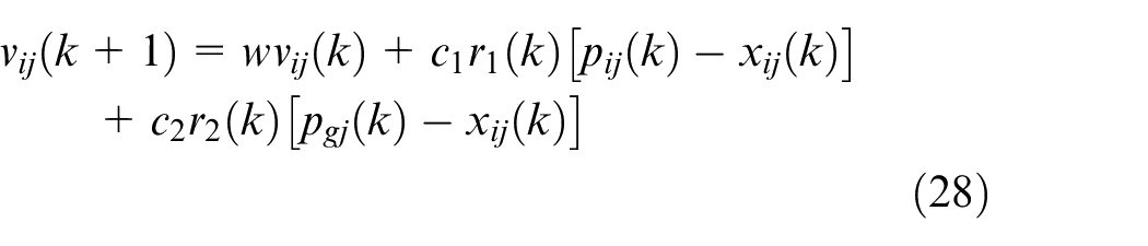
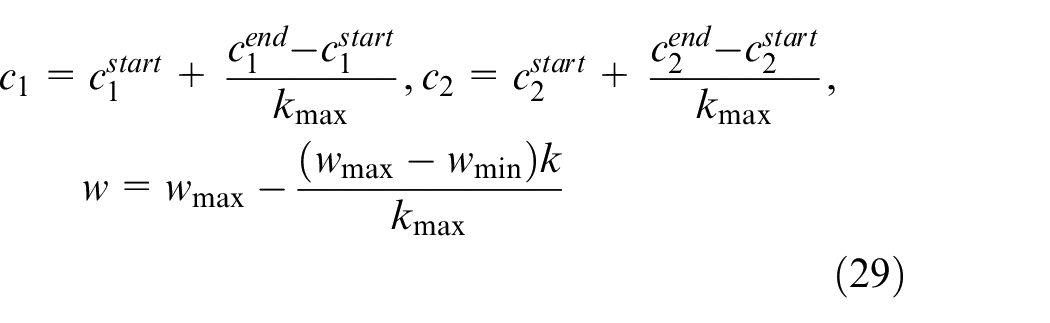
Where (27)−(29): k is the iterations number, r1(k) and r2(k) are [0,1] uniformly distributed random numbers, pij(k) and pgj(k) are the local optimums and global extremes found by the particles during the iterative process. Among them
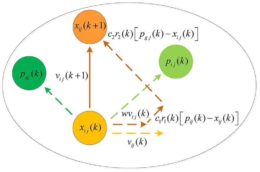
Particle position and velocity update map.
In this paper, the time multiplied absolute error integration criterion (ITAE metric) is selected as the fitness function for the optimization of FUZZY-PID and PID controller factors:
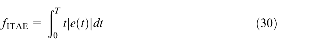
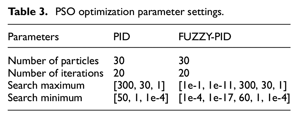
Table 3 shows the specific parameter values set for the PSO in this paper.
PSO optimization parameter settings.
For the parameters and the optimization constraints of the model are as follows:
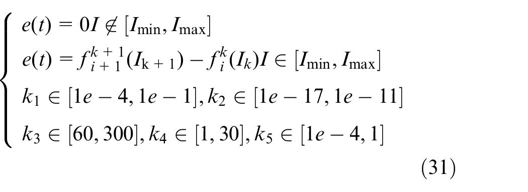
Where
Combined with Table 3, Figure 9 shows the PSO optimization controller factor flow.
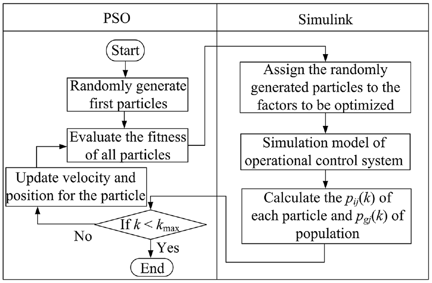
PSO-optimized controller flow chart.
As shown in Figure 9, the algorithm first generates a random set of particles, evaluates the fitness of particles, assigns the generated particles to the factors to be optimized, then run the simulation model, and the particles are searched for optimality in the solution space. During the iteration, calculate pij(k) and pgj(k) and compare them with historical values to find the optimal value. Until the termination condition is satisfied, pij(k) and pgj(k) both follow equations (27)–(29) to continuously update the particle velocity and position.
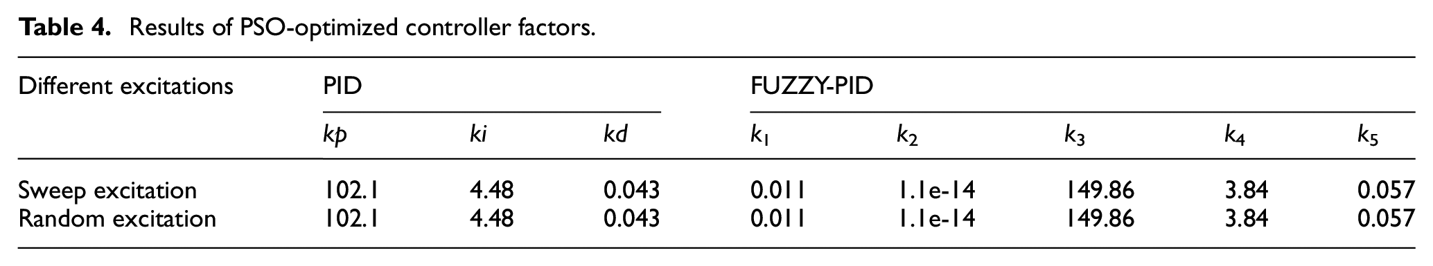
Table 4 shows the results of the optimization factors for PSO under different excitations.
Results of PSO-optimized controller factors.
Simulation results of self-tuning control algorithms under different excitations
Determine the self-tuning control algorithm
The STMFRBD intrinsic frequency studied in this paper 30 :
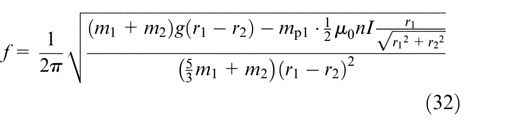
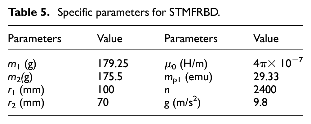
It can be seen from equation (32), f is related to the parameters m1, m2, r1, r2, n, I, etc. Table 5 shows the values of some parameters of equation (32).
Specific parameters for STMFRBD.
By substituting the values of Table 5 in equation (32), the frequency can be rewritten as:

Combining equation (33) and the parameters in Tables 1 and 5, the stiffness, damping, and frequency of the damper can be obtained as a function of current, and the results are shown in Figure 10.
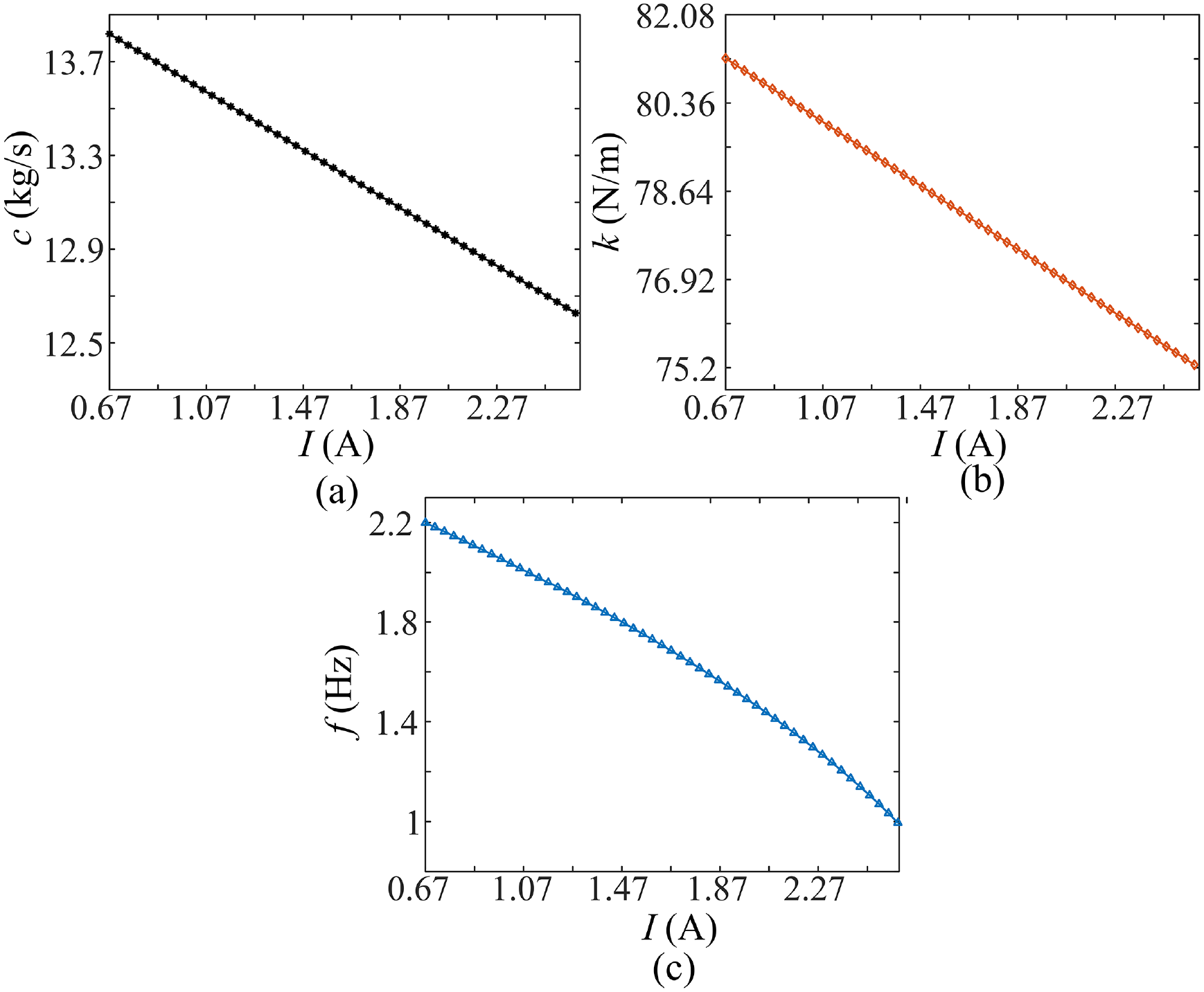
Variation of damper parameters with current: (a) damping, (b) stiffness and (c) frequency.
From Figure 10, when the electric current I varied in the range of 0.67–2.6 A, the damping coefficient of the damper varies in the range of 12.64–13.82 kg/s, the stiffness coefficient varies in the range of 75.2–81.22 N/m, and the intrinsic frequency f of the damper changes in the range of 1–2.2 Hz. That is, when the current changes in a certain range, the relevant parameters of the damper are changed, among which the intrinsic frequency changes the most. Therefore, the optimal damping of the damper can be achieved by adjusting the inherent frequency of the damper.
This paper compares PID, PSO-PID, FUZZY-PID, and PSO-FUZZY-PID to tune the damper frequency by tracking the excitation frequency under the sweep and random excitation. The optimal algorithm is selected as the frequency tracking control algorithm based on the stability, tracking accuracy, and the presence or absence of down-shoot and overshoot of the four control algorithms.
Sweep signal variations
The excitation frequency is continuously varied from 1.0 to 2.2 Hz in 0 to 40 s and is used as the reference signal (REFS). From equation (33), when the electric current I is 0, the frequency is 2.5 Hz. Therefore, when the algorithm causes an overshoot of 2.5 Hz at 0 s regulation, it can default as not caused by the algorithm performance, that is, it is not considered an algorithm performance indicator. The next comparison of four different control algorithms to tune the damper’s frequency tracking REFS is shown in Figure 11.

Simulation of sweep frequency change tracking control.
From Figure 11, in the initial state, the PID control produces an overshoot of nearly 3 Hz and a down-shoot of 0.18 Hz, which stabilizes at 2.3 ms. The FUZZY-PID control does not produce overshoot and down-shoot but produces an error of 5% with REFS, which stabilizes at 50 ms. The PSO-PID control produces an overshoot of 2.6 Hz and a down-shoot of 0.18 Hz, which stabilizes at 4.2 ms. The PSO-FUZZY-PID control not only generates no overshoot and down-shoot but accurately tracks the vibration frequency and achieves stability in 7.15 ms compared to FUZZY-PID, shortening the time to stability.
Random signal variations
Figure 12 shows the excitation frequency randomly changing every 4 s at 1.0–2.2 Hz as the reference signal (REFS), comparing the four control algorithms to tune the damper’s frequency to track the REFS change.
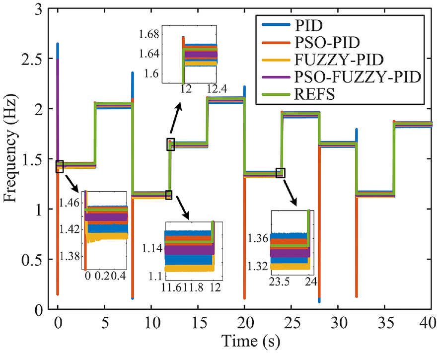
Simulation of random frequency tracking control.
From Figure 12, the PID tune frequency with an overshoot of 2.68 Hz and a down-shoot of 0.15 Hz, stabilizes at 2.8 ms and produces varying degrees of down-shoot and overshoot at most subsequent frequency changes. The PSO-PID tunes the frequency without overshoot, but generates a down-shoot to 0.095 Hz, stabilizes at 8.2 ms, and generates varying degrees of down-shoot and overshoot at subsequent frequency changes. The FUZZY-PID tunes the frequency without down-shoot and overshoot, but generates an error of 0.04 Hz at the beginning, stabilizes at 32 ms, and generates varying degrees of error in the subsequent tune time. PSO-FUZZY-PID without down-shoot and overshoot, and compared with the first three algorithms not only can accurately track the change of REFS but can greatly reduce the time to reach stability.
From Figures 11 and 12, when tracking different excitation frequencies, the frequency tracking different control algorithms are different. The PID has overshoot and down-shoot at some track-up points, while the PSO-PID has a large down-shoot and long stabilization time, and the FUZZY-PID has no down-shoot or overshoot but generates large errors and takes a long time to stabilize. PSO-FUZZY-PID not only has no down-shoot and overshoot but can reach stability quickly and track REFS accurately, so PSO-FUZZY-PID is selected as the self-tuning algorithm.
Comparison of vibration reduction between STMFRBD and PMD
Based on the kinetic equations (15)–(16) in Section 2.1 and the PSO-FUZZY-PID designed in section 3, the system dynamic response under different excitations is simulated using MATLAB software. To demonstrate the superiority of STMFRBD, the dynamic response of STMFRBD, PMD, and the system without dampers are compared, to compare the STMFRBD and PMD damping performance. Considering sweep and random excitation conditions, the PMD damping band is set near the system resonant frequency and kept constant.
System response under sweep excitation
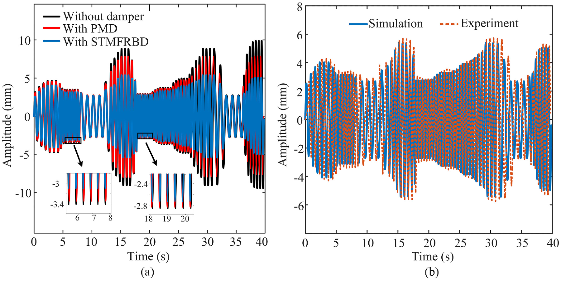
The excitation amplitude is set at 2 mm and the frequency is continuously varied from 1.0 to 2.2 Hz in the period of 0–40 s. Figure 13(a) shows the dynamic response of the system under simulation by applying MATLAB. Figure 13(b) shows the comparison of the dynamic response under STMFRBD simulation and experiment.
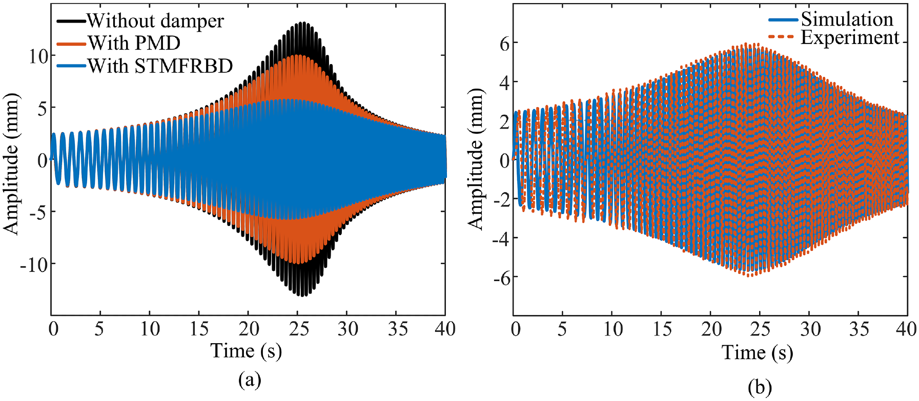
Sweep excitation: (a) dynamic amplitude response and (b) comparison of STMFRBD simulation experiments.
From Figure 13(a), the amplitude response of the three curves tends to increase and then decrease with the increase of the excitation frequency. Before 25.5 s, the amplitude response of the three different operating conditions gradually increases, and after 25.5 s, it gradually decreases. The amplitude response of the system without dampers reaches 13.07 mm at 25.5 s, while the amplitude response of the system with PMD and STMFRBD is 9.92 and 5.67 mm, respectively, which is because STMFRBD can tune its intrinsic frequency in real-time to achieve tuned damping. The PMD only achieves a good damping effect near the resonance point and shows poor damping performance far from the resonance point. As shown in Figure 13(b), two curves coincide as a whole, and the average error of the response amplitude of both is 5.17%, verifying the theoretical model accuracy.
The damping effect of the system under the action of PMD and STMFRBD is quantitatively described using the following equation:
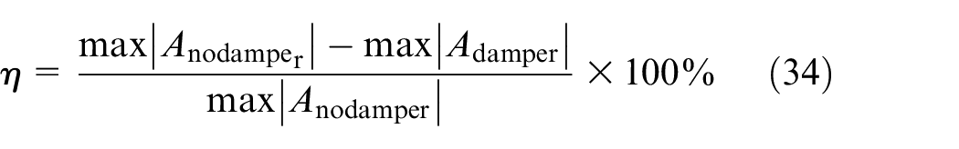
Where
The system amplitude response time, is divided into eight segments, and the average response amplitude of the system is calculated for each segment of the damper action respectively, and Table 6 shows the vibration reduction rates of different dampers calculated using equation (34).
The vibration reduction rate of different dampers under sweeping load.
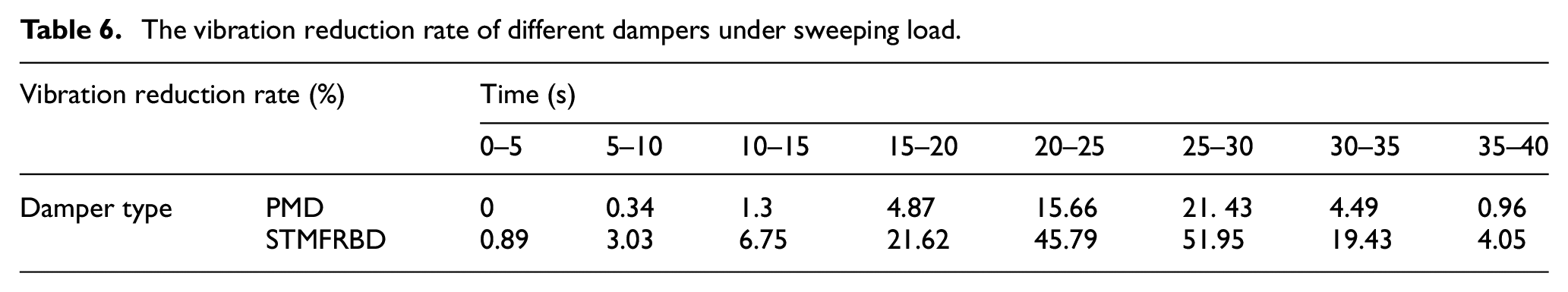
As shown in Table 6, the STMFRBD average vibration reduction rate is 19.18% compared to 6.13% for PMD, indicating that STMFRBD has better damping performance compared to PMD.
System response under random excitation
The excitation amplitude is set at 2 mm, and its frequency varies randomly every 4 s between 1.0 and 2.2 Hz. Figure 14(a) shows the dynamic response of the system under simulation by applying MATLAB. Figure 14(b) shows the simulation and experimental comparison of STMFRBD under random excitation.
Random excitation: (a) Dynamic amplitude response and (b) STMFRBD simulation experiment comparison.
From Figure 14(a), the system response amplitude is different under different excitation amplitude responses. The PMD reduces the amplitude to 6.66 and 6.85 mm at 12–16 s and 36–40 s, respectively, while the STMFRBD reduces the amplitude to 4.62 and 4.42 mm. Figure 14(a) shows that STMFRBD still shows a good frequency tracking effect under random excitation and exhibits superior damping performance. From Figure 14(b), the two coincide as a whole, where the maximum error is 6.69%, verifying the theoretical model accuracy.
From Figure 12, random excitation involves eight different frequencies, and Table 7 shows the damper’s vibration reduction rates calculated for eight different random frequencies in combination with equation (34).
Vibration reduction rates of different dampers under random loading.
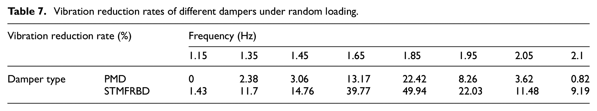
The simulation results of combined sweep and random excitation show that STMFRBD has better overall damping performance than PMD. This is because the PMD intrinsic frequency cannot be tuned, and when the excitation frequency changes, the PMD damping effect will be weakened. In contrast, STMFRBD can track the external vibration frequency to tune its intrinsic frequency to achieve tuned damping, so that the structure is in the optimal damping state.
Experimental research
To verify the damping performance of STMFRBD, this section compares and analyzes the vibration-damping performance of PMD, TMFRBD, and STMFRBD through experimental test methods, where the PMD mass is equivalent to a rolling-ball with built-in MF. Using free vibration decay experiments, the intrinsic frequencies of the structure and the dampers can be measured before and after the application of the dampers. Then according to the different vibration modes, the vibration damping performance test experiments are divided into swept load and random load vibration experiments. Since the structural response under both experiments is a non-stationary signal, the paper uses the Hilbert-Huang et al. transform (HHT) to perform a time-frequency analysis of the non-stationary signal of the response.36,37
Experimental program design
The experiment uses a single-degree-of-freedom frame to simulate the structure for vibration damping experiments, and the frame stiffness and damping coefficients are 979.4 N/m and 16.9 kg/s, the structural height is 465 mm and remains constant during sweeping and random load vibration. The free vibration decay experiment is an experiment to test the structure and the dampers’ natural frequencies by applying a fixed displacement offset of 12 mm to the top of the structure without external excitation. Sweeping frequency load vibration experiments use an electromagnetic shaker to apply a constant amplitude and continuously varying frequency to the structure. The front contact of the electromagnetic shaker is connected to the structure before the experiment, the signal generator controls the excitation frequency and excitation displacement of the shaker. The random load vibration experiment is a computer-side controlled shaker that produces a vibration with constant amplitude and randomly varying excitation frequency. The same platform is used for both experimental tests, and the test platform is built as shown in Figure 15(a). The TMFRBD used for the experiments is shown in Figure 15(b).
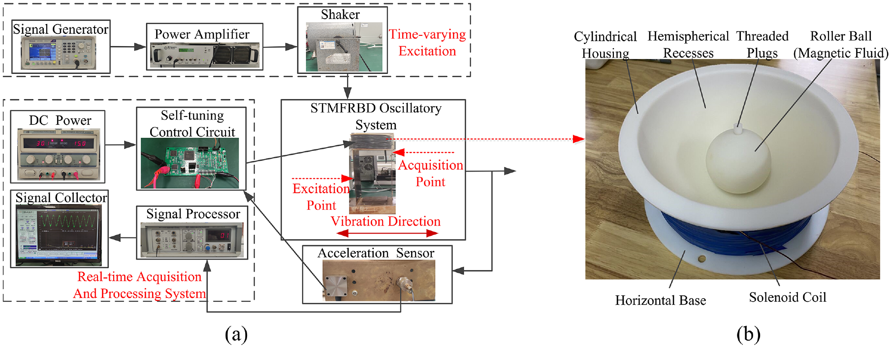
Experimental setup: (a) test platform and (b) TMFRBD.
As known from Figure 15(a), the experimental platform involves experimental devices mainly including a signal generator, power amplifier, signal processor, shaker, STMFRBD vibration system, self-tuning control circuit, DC power supply, acceleration sensor, etc. Among them, the STMFRBD vibration system consists of a single free frame structure and STMFRBD, and the MF (provided by Beijing Shenran Magnetic Fluid Company) is a kerosene-based ferric tetroxide MF with a density of 1.76 g/cm3. Two acceleration sensors are connected to the top of the structure. One acceleration sensor transmits the collected vibration signal directly to the self-tuning control circuit, which calculates and identifies the structural vibration main frequency, and then outputs the corresponding electric current signal to tune the intrinsic frequency of the damper. The other acceleration sensor transmits the collected vibration signal through the signal processor to the DASP software system on the computer side of the signal collector, which automatically converts the acceleration signal to a displacement signal and can monitor the structural amplitude response in real-time.
From Figure 15(b), the TMFRBD contains a hemispherical recess, a ball (MF), a solenoid coil, etc. The damper’s intrinsic frequency can be tuned by electric current. Since the hemispherical recess is rigidly connected to the structure and only provides a moving environment for the ball, namely the damping effect is played by the ball and the MF, so the no-damper mentioned in the text refers to no ball and MF. Since the mass of the ball and the MF are small compared to the structure, they do not affect the characteristics of the structure such as the intrinsic frequency.
Free vibration decay experiment
By using a 12 mm fixed displacement offset method, the free vibration decay frequencies of the structure before and after the application of the damper can be measured separately, where the intrinsic frequency of the structure can be changed by adjusting the height. In this section, the frequencies of STMFRBD and the structure are tested, and the structure is adjusted at 485 and 434 mm, and the measured free decay vibration frequencies are 1.65 and 1.85 Hz. The top amplitude response of the structure without dampers and STMFRBD is shown in Figure 16.
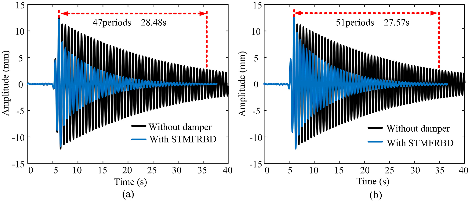
Free vibration decay experiment: (a) 1.65 Hz and (b) 1.85 Hz.
From Figure 16, it can be seen that the structure and STMFRBD move for 47 and 51 periods in 28.48 and 27.57 s, corresponding to the intrinsic frequencies of the structure at two different heights, that is, 1.65 and 1.85 HZ, respectively. The structure height is adjusted several times to measure the inherent frequency of the structure at different heights. Under the condition of satisfying the tuned vibration reduction, the magnitude of the tuning electric current required for STMFRBD to track the frequency change of the structure at different heights can be calculated by combining equation (33), respectively. The frequency and electric current data of the structure and STMFRBD are shown in Table 8.
Experimental results of free vibration decay.
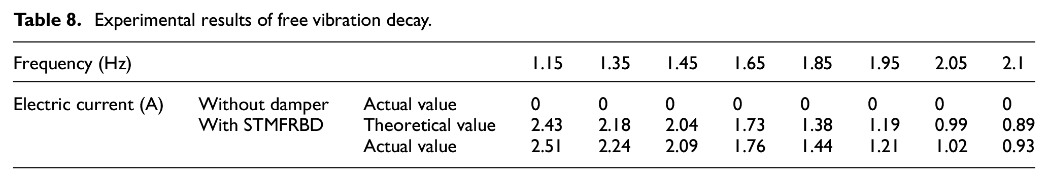
From Table 8, STMFRBD can adjust its own inherent frequency with the inherent frequency of the structure by electric current. The maximum error between the theoretical and actual values is 4.49%, which is within the allowed error range and can meet the experimental requirements.
Sweeping load vibration experiment
First set the excitation displacement of the shaker to 2 mm, and then set the signal generator to generate a 1.0–2.2 Hz sine sweep signal in 0–40 s, and use the signal collector to collect the structural top amplitude in three different cases of PMD, STMFRBD, and no damper, which can be obtained as the curve shown in Figure 17(a). The three curves in Figure 17(a) are expanded separately and the time-frequency analysis of the three curves is performed using HHT, and the curve shown in Figure 17(b) can be obtained. Then divide the 40 s time of amplitude response of Figure 17(a) into eight segments equally, and calculate the vibration reduction rate under each segment separately by combining with equation (34), the curve shown in Figure 17(c) can be plotted.
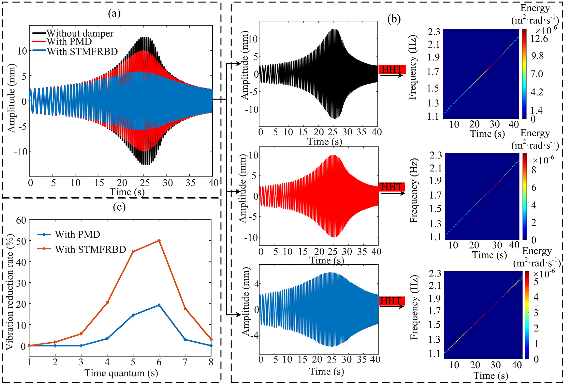
Structural response under sweeping excitation: (a) Structural amplitude response with different dampers, (b) time-frequency analysis, and (c) comparison of vibration reduction rates of two dampers.
From Figure 17(a), the structural top amplitude shows a trend of increasing and then decreasing. When the structural intrinsic frequency and the excitation frequency are equal, the structural amplitude reaches 12.6 mm without dampers, while PMD and STMFRBD can reduce the structural amplitude to 9.2 and 5.72 mm, respectively. From Figure 17(b), the output signal’s main frequency is the same as the excitation frequency (1.0–2.2 Hz), where the vibration energy is mainly distributed around the resonance frequency. Since the damping frequency band of PMD is near the structural intrinsic frequency, it cannot change its intrinsic frequency. Therefore, the vibration energy distribution in the time-frequency diagram is similar to that of the structure without dampers, with only an energy reduction. The STMFRBD can track the structure vibration frequency, therefore, its vibration energy distribution is not only lower but more uniform compared to that of the unhampered PMD. As shown in Figure 17(c), the vibration reduction rate in both operating conditions tends to increase first and then decrease. The vibration reduction rate in the sixth period reaches 19.26% and 50.05% for the two operating conditions, respectively. During the whole period, the average vibration reduction rate of PMD is 5%, while the average vibration reduction rate of STMFRBD is 17.99%. On the whole, the damping effect of STMFRBD is better.
Random load vibration experiment
Firstly, the excitation displacement of the shaker is set at 2 mm, and the signal generator is used to generate the excitation frequency with random distribution at 1.0–2.2 Hz every 4 s. Figure 18(a) shows the amplitude response of the PMD, STMFRBD, and no damper at the top of the structure collected by the signal collector. Figure 18(b) shows the time-frequency analysis of the three curves of Figure 18(a) using HHT respectively. From Figure 18(b), eight different frequencies vary randomly. The amplitudes at different frequencies are averaged and the vibration reduction rates at different frequencies are obtained using equation (34) to plot the curves shown in Figure 18(c).
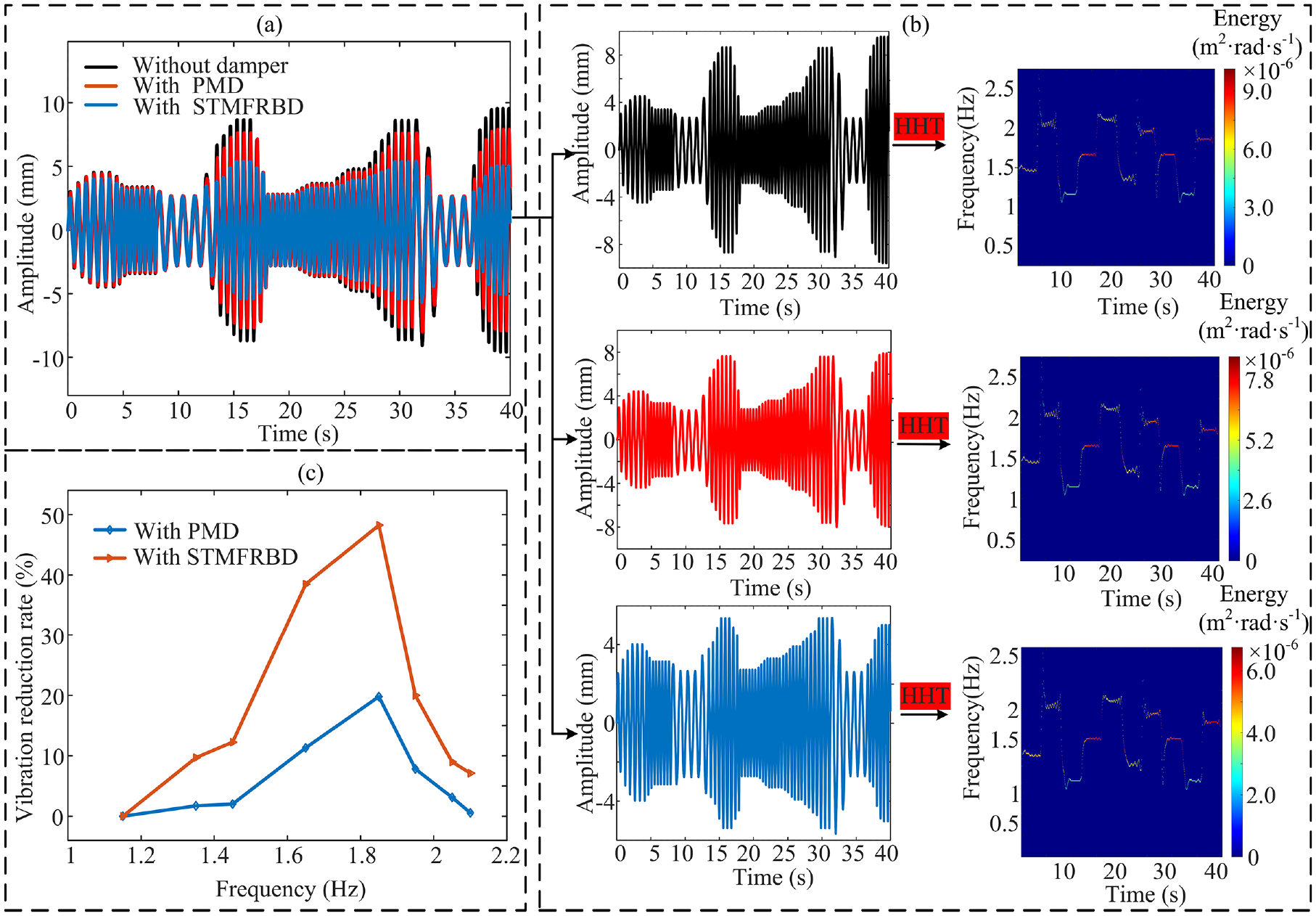
Structural response under random loading: (a) structural amplitude response with different dampers, (b) time-frequency analysis, and (c) comparison of vibration reduction rates of two dampers.
From Figure 18(a), the structural amplitude response is different at the corresponding frequencies for each period. The structural amplitudes without dampers reached 7.51 and 8.54 mm at vibration frequencies of 1.65 and 1.85 Hz, respectively. PMD and STMFRBD reduced the structural amplitude to 6.66 and 4.62 mm, respectively, at a vibration frequency of 1.65 Hz. PMD and STMFRBD reduced the structural amplitude to 6.85 and 4.42 mm, respectively, at a vibration frequency of 1.85 Hz. From Figure 18(b), the structural vibration energy is mainly distributed around the resonance frequencies of 1.65 and 1.85 Hz. When there is no damper, the structural vibration energy is highest at these two frequencies. When the PMD acts, reducing the structural vibration energy by 11.66% and 17.38% at these two frequencies, respectively, however, at other frequencies, there is a maximum reduction of 4.79%, and the lowest is unchanged. When STMFRBD is applied, the structure not only reduces the vibration energy by 37.99% and 47.43% at these two frequencies but reduces the vibration energy by different degrees at other frequencies.
From Figure 18(c), the damping effect of STMFRBD is higher than that of PMD. When the vibration frequency is 1.85 Hz, the vibration reduction rates of the two operating conditions reach 19.79% and 48.24%, respectively. When the vibration frequency is 1.95 Hz, the vibration reduction rate of STMFRBD is still 20%, but the vibration reduction rate of PMD is 7.83%. This is because the damping band of PMD is narrower, and cannot be changed when the excitation frequency is changed, so it can only have a certain damping effect near the resonance frequency. In contrast, the STMFRBD proposed in this paper can track and collect the structural vibration frequency, and even under complex excitation, it shows better frequency tracking stability and real-time adjustment of the intrinsic frequency in line with the excitation frequency to achieve the optimal reverse resonance.
Comparison of STMFRBD and TMFRBD under different loads
Considering the frequency of random loads and the damping effect of TMFRBD at 1.45, 1.65, 1.85, and 1.95 Hz frequencies are more representative, this subsection will compare the damping of TMFRBD at four frequencies with STMFRBD and PMD at different loads. The vibration reduction rates of the dampers under different loads can be obtained by combining equation (34), as shown in Figure 19.
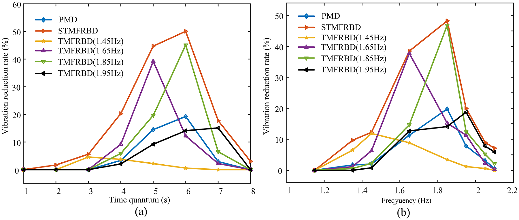
Comparison of damping rates for different load dampers: (a) sweeping load and (b) random load.
From Figure 19, when the intrinsic frequency of the STMFRBD tracks the external excitation change under different load experiments, some band ranges of its regulation will cover TMFRBD with different frequencies. Therefore, when the frequency point of TMFRBD appears near the regulation band of STMFRBD, it will be close to the damping rate of STMFRBD, which is the reason why the highest point of the damping rate curve of TMFRBD with different frequencies is similar to that of STMFRBD. However, the damping effect of TMFRBD is poor at other excitation frequencies, sometimes even lower than PMD, because the inherent frequency of TMFRBD cannot track the change in excitation frequency. The average damping rates of PMD and STMFRBD under sweeping load vibration are 5% and 17.99%, respectively, while the highest average damping rate of TMFRBD is 9.64% and the lowest is 1.39%. In summary, the damping effect of STMFRBD is better than that of PMD and TMFRBD under time-varying excitation.
Conclusion
An accurate and efficient self-tuning control algorithm is the prerequisite and key to ensuring the damping effect of TMFRBD under complex external excitation. In this paper, a self-tuning control algorithm is proposed by combining the operating characteristics of the TMFRBD, namely Particle Swarm Optimization (PSO)-FUZZY-PID. To evaluate the proposed control algorithm performance quality, the frequency tracking and damper’s damping effect under different working conditions through simulation and experiment have been studied.
The variation of dynamic amplification factor under different parameter schemes is compared. The results show that for structural vibrations under time-varying excitations, the defect of the narrow damping band of conventional passive dampers is compensated by the frequency tracking scheme with Z = 1, and the damping performance of the dampers is greatly improved compared with that of unoptimized and parameter-optimized passive dampers.
Comparing the proposed self-tuning PSO-FUZZY-PID with PID, PSO-PID, and FUZZY-PID control algorithms in different operating conditions where the damper’s frequency tracks the change of excitation frequency, the results indicate that the PSO-FUZZY-PID can stably, quickly, and accurately tune the damper’s frequency to track the change of external excitation frequency compared with other algorithms.
The simulations and experimental comparisons of the vibrating structure with attached STMFRBD are carried out under different excitations, verifying the dynamics model accuracy. The maximum vibration reduction rates of STMFRBD, PMD, and TMFRBD under different excitations are 51.95%, 21.43%, and 45.1%. The average damping rates of PMD and STMFRBD under sweeping load vibration are 5% and 17.99%, respectively, while the highest average damping rate of TMFRBD is 9.64% and the lowest is 1.39%. The proposed STMFRBD can be selected as the dampers for towering structures in the engineering field.
This paper proposed the damper self-tuning control algorithm which can be used for the rolling-ball damper to track the frequency under time-varying excitation, which paves a new way to design frequency tracking schemes and control algorithms of the other tuned dampers.
Footnotes
Declaration of conflicting interests
The author(s) declared no potential conflicts of interest with respect to the research, authorship, and/or publication of this article.
Funding
The author(s) disclosed receipt of the following financial support for the research, authorship, and/or publication of this article: This work was supported by the National Natural Science Foundation of China under Grant No. 51877066.