
Abstract
We describe an asymptotic method for calculating the size of a zone of partial slip at the edge of a complete contact of arbitrary edge angle and coefficient of friction. Above a critical coefficient of friction the contact remains stuck, and this critical value is explored. A distributed dislocation method is used and the use of different types of numerical quadrature is explored. The size of the slip zone, and its dependence on the contact edge angle and coefficient of friction, are explored.
Introduction
A complete contact is one whose extent is defined by a discontinuity in the gradient profile of one of the contacting surfaces. In layman’s terms, this means that the edge of the contact is located at the corner of either of the contacting bodies. This gives rise to a stress singularity at the edge of the contact1–3 provided that the contact remains intimate throughout the initial contact region, that is, the loading is such that the corner does not lift off. The singularity has to be relieved, and this can be done by plasticity, 4 by the nucleation and propagation of cracks, 5 or by local frictional slip along the contact interface. This contact may persist across then entire interface (i.e. two separate bodies in contact), or it may be a closed pair of crack faces, 6 we consider the former in this case.
It is the last of these effects which we will consider here. The creation of a zone of partial slip is dependent on the loading, as described by Riddoch and Hills 7 the intimate contact must be maintained by the correct signs of the stress intensity factors, and as laid out by Hills and Dini 8 the coefficient of friction must be lower than the value of the traction ratio implied within the dominant eigenvector of the Williams solution. 9
Calibrations of external loads to the stress intensity factors have shown that the contact will tend to spread outwards under purely normal loading,7,10,11 so initial investigations focus on outward slip.
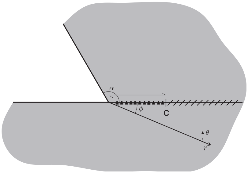
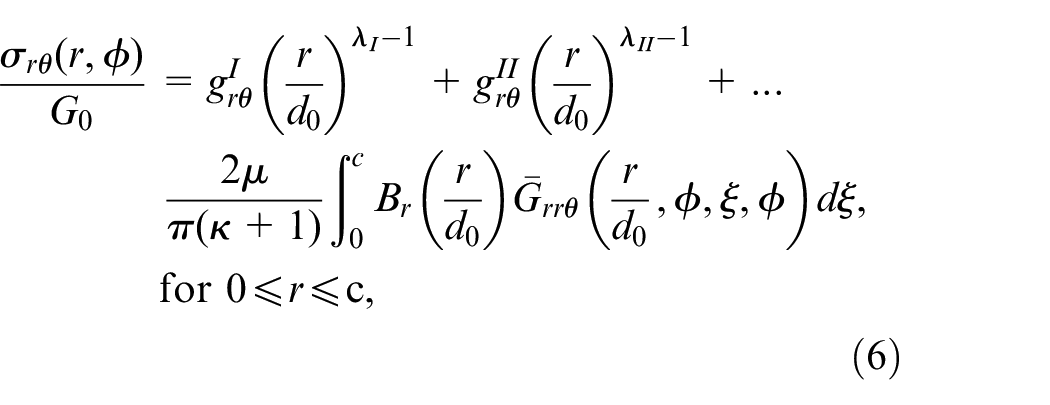
Applying Coulomb’s friction law throughout, this analysis will endeavour to model the slip and determine the size of the slip zone. Furthermore, previous work has considered only the three-quarter plane problem,12,13 which applies, for example to the problem of a square block indenting a half-space. In this analysis, this will be extended to consider a variety of indenter angles. Additionally, previously it has been stated that the size of the slip zone, when normalised by a value calculated from the Williams solution, is independent of the coefficient of friction, which has now been found to be incorrect. Figure 1 shows a sketch of the resultant system, with the slip zone present at the edge of contact.
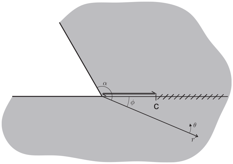
Sketch of a slip zone at the edge of a complete contact of arbitrary internal angle.
Asymptotic formulation
It has already been mentioned that the Williams solution9,14 will be used extensively. This provides an asymptotic solution to determine the state of stress in the neighbourhood of the apex of a wedge. This solution places the origin of a polar coordinate system at the edge, a feature which is preserved throughout this analysis.
The state of stress is dominated by two terms, which are the symmetric (here after referred to as mode I) and anti-symmetric (hereafter referred to as mode II) eigensolutions. For a wedge having total internal angle greater than
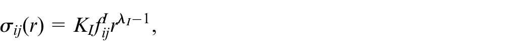
The stress is described by the formula
where
This solution may be used as a bilateral solution, as an adhered complete contact is equivalent to a wedge whose internal angle is the sum of a half-plane and the internal angle of the contacting body. Therefore, this solution can be used as the basis for this analysis. At this stage, we will define two constants, that we find from the Williams solution and which will be useful later.
We begin by recalling the work of Hills and Dini
4
and using this to extract the characteristic length dimension of the problem. Before doing this, however, it will be useful to align the eigensolution of the problem to the slip line with new basis vectors along the interface, as this will allow easier normalisation later on. Quite simply this is done by applying multipliers to the vectors;
The second important quantity we wish to define is the implied size of the slip zone, as indicated by the ratio of the tractions given by the Williams solution. This is the point where
where
Finally, we will use our inherent length scale (

Dislocation formulation
Turning now to the problem of modelling the actual extent of slip, we require a knowledge of the size of the slip zone, and a method of modifying the stresses. The former will be something we will return to later, but for the latter, we will use dislocations. Crystalline dislocations are used in material science to represent discontinuities in lattice structures, although that is not how we will use them here.
Instead we are interested in the stress and displacement fields that the dislocations create. The form of these is well known and understood15–18 and will be used extensively. These influence functions are known for a dislocation in an infinite plane, and so a method must be found to determine the influence of such dislocations in a semi-infinite wedge, a system which, as we have said, is analogous to an adhered complete contact. This has been done previously by considering a single dislocation and using distributions of dislocations to clear the free surfaces of induced traction,19–22 and in this analysis we will use the results calculated by Riddoch and Hills. 22
Denoting the wedge influence of a dislocation by
Sketch showing the distribution of dislocations along the slip interface.
Consequently, the corrected stresses along the contact interface can be written as
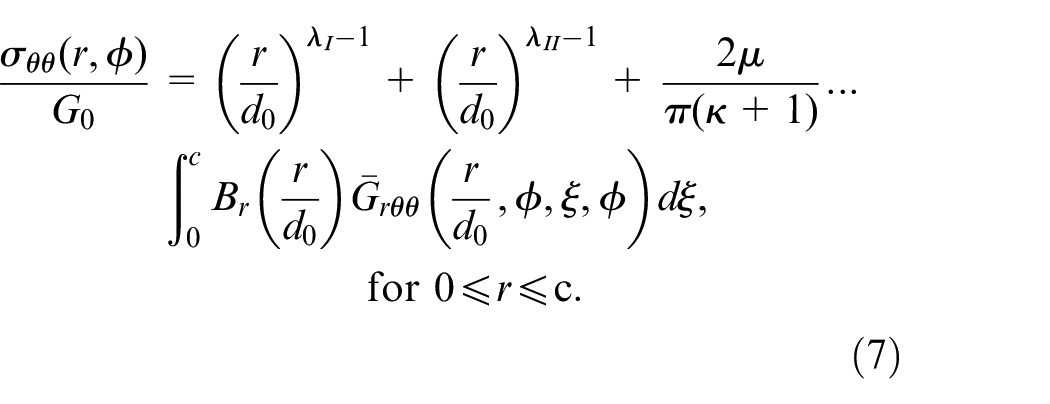
Within the slip region, the Coulomb friction law must be satisfied, meaning
where
A numerical inversion
Considering, first, the inversion of the integral equation, we note that we will require a numerical method. This is because the dislocation kernels, as found by Riddoch and Hills 22 do not have a closed-form expression. The kernels are, however, singular in nature, so equation 8 is a Cauchy singular integral equation.
Numerical quadrature
Consequently, a Gauss-Chebyshev quadrature will be employed as described by Erdogan et al.
23
This quadrature deals with the singularity by separating the behaviour into a well-behaved unknown function, denoted by
The choice of this fundamental function determines the type of behaviour that can be expected of the solution at the end points. However, there are only two types of behaviour which are accounted for, square root singular, and square root bounded, and so with either possible at both ends, giving a total of four different cases, as laid out in Table 2.2 by Hills et al. 24
We must consider the state of stress at the edge of contact and the slip stick boundary. Considering, first, the latter, in the adhered case, the stress at this point is bounded, with each component’s value being a finite number, this will still be true as the contact slips. So here the corrective term must be bounded.
The question is not so easily resolved at the contact edge end of the interval however. The stresses in the bilateral solution are singular at the edge of contact, specifically, they are power order singular, and the power is given by
Applying singular-bounded quadrature
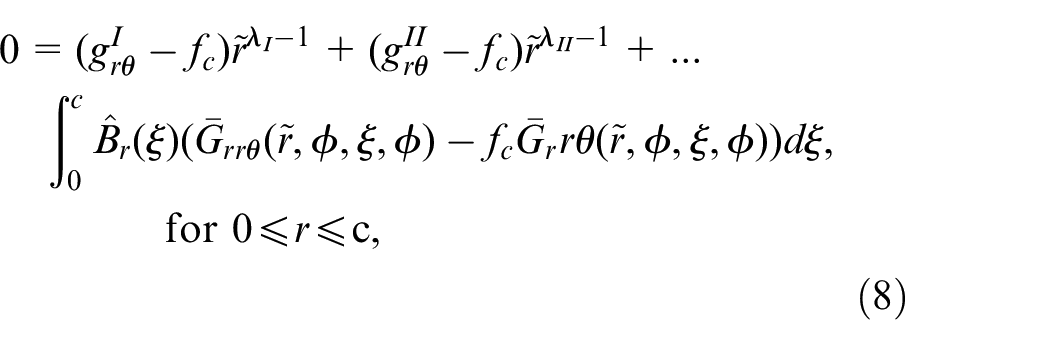
Consequently, a singular-bounded quadrature is employed. It should be noted that this is the same quadrature as was applied by Churchman and Hills. 12 Table 2.2 (case II) in Hills et al. 24 then gives us a method for choosing our collocation and integration points.
Before we can apply the quadrature, we must first transform the integral. The quadrature requires the integration range to be
Applying these substitutions gives us the integral equation
At this point it is worth noting that generally
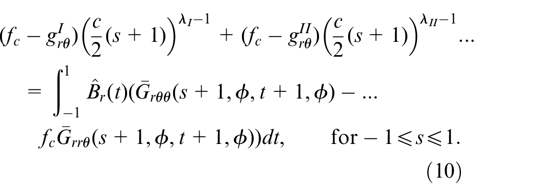
This equation is now in a form where the quadrature may be applied. This leads us to a set of
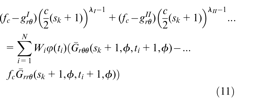
where
The size of the slip zone
Having in hand this inversion method, we now come to solve the set of equations. By use of the transforms, this requires knowledge of the size of the slip zone
Two constraints
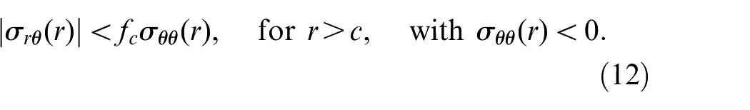
Previous studies12,13 have utilised a pair of conditions to calculate the size of the slip zone. This is done by guessing the size of the slip zone, and then checking these conditions to ensure that the estimated slip zone size satisfies both.
These conditions are derived from two basic phenomena. The first of these is that Coulomb’s law is satisfied at a given point if and only if the point is in the slip region. For a point within the slip region, as specified by equation 8, this condition will be automatically satisfied by any solution to equation 8. Points outside of the slip zone satisfy this condition:
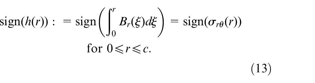
The second condition within the slip region is derived from the orthogonality condition. This requires the velocity of a slipping point to have the same sign as the shear stress at that point. As this analysis is quasi-static in nature, we do not have a rigorous definition of velocity. However, it is a sufficient approximation to consider instead the slip displacement. Slip displacement is defined as the integral of the dislocation density, since the dislocations themselves represent the displacement discontinuity. We may write this condition as
We now have four conditions, summarised in Table 1. The first of these, condition A, is automatically enforced by the solution of the integral equations. Similarly, the last of these, condition D, is automatically true; no dislocations are present along the interface in the stick region and so no displacement is caused. We can, however, use the remaining two conditions, B and C, to constrain the solution. These place restrictions on the solution in the slip region and the stick region, and it may appear that these conditions are sufficient.
Table of conditions in the slip and stick regions.
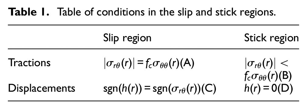
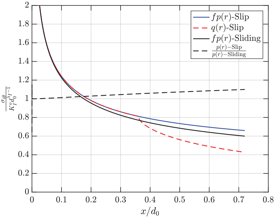
Experience has shown that in this case, the conditions, whilst necessary, are not sufficient to define a unique size for the slip zone. Figure 3 shows the stresses implied by a slip zone which is too small, according to our findings later in the “Results” section. It can be observed that both conditions described here are satisfied, the left hand plot shows (solid black line) that no slip is implied in the slip region. Furthermore, it can easily be observed that both the shear traction (solid red line) and the slip displacements(right hand plot) are positive throughout the slip zone. This would therefore appear to be a valid solution.
Plot of the stresses in a slipping square edge indenter with a slip zone of size
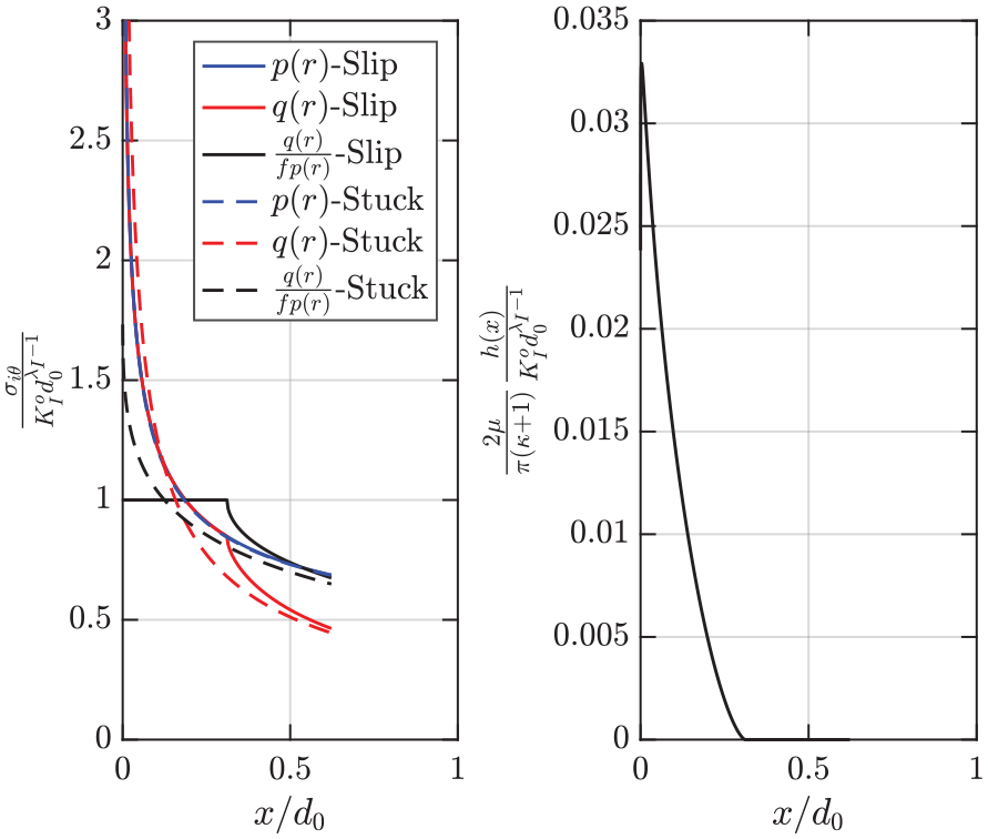
Figure 4 shows the stress in the same contact, but in this case we specify a slip zone size that we believe to be too large. Once again, it can be observed that there is no violation of the slip condition in the stick region (solid black line, left hand plot) and that slip displacement and shear stress have the same sign (right hand plot and solid red line, left hand plot respectively.) So this too would appear to be a valid solution.
Plot of the stresses in a slipping square edge indenter with a slip zone of size
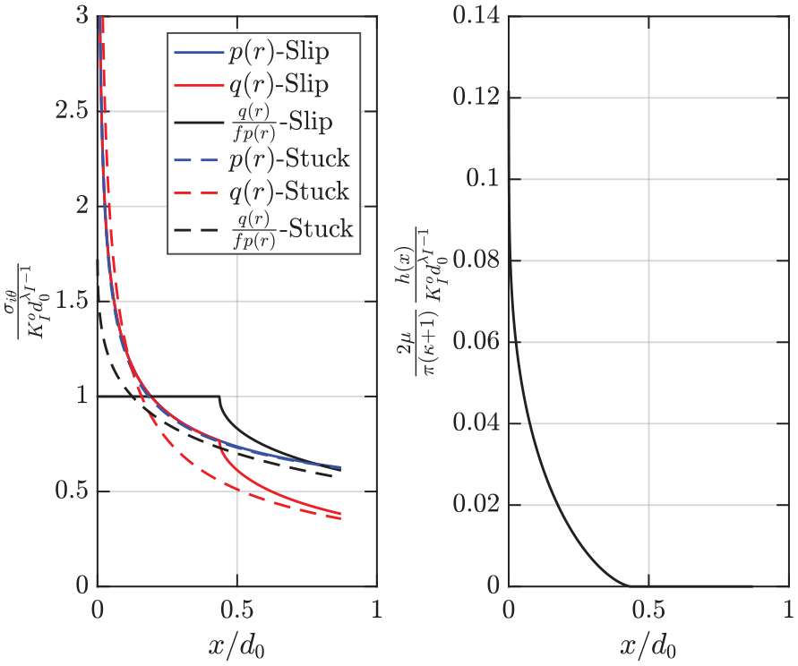
This is obviously problematic, the constraints are not only providing multiple solutions, but rather a range. Experience shows for example that for
Overlay plot showing the stresses produced for two different slip zone sizes, small being
The sliding solution
As previously mentioned by Churchman and Hills
12
it may be useful to consider the solution for a sliding block, as developed by Conminou.
25
This gives rise to an eigenvalue, denoted

However, the sliding asymptote is valid only for a very small region of the slip zone. We do not have to hand, a bound of the range of validity of this solution, so we cannot say with any confidence that this approximation will be accurate at any point a finite distance from the contact edge. The solution is exact only when
Slip displacements
The orthogonality condition requires the calculation of the slip displacements, which must be of the same sign as the shear stress. It is tempting to find other conditions. Perhaps the most obvious of these to consider is the prevention of a turning point in the slip displacements. Intuitively it may seem that the slip displacements must be strictly increasing from the slip stick boundary to the edge of contact.
However, this statement has been made without justification, and no immediate justification is apparent. Slip displacements are calculated from dislocation densities, and hence reference discontinuities, so no relation between the stress and the strain may be drawn. So, whilst it may appear at first sight to be obvious, we cannot say with any certainty that this will be the case, and so we can not enforce a condition based on this assumption.
Similarly, it could be argued that the slip displacement should not show singular behaviour at the edge of contact either. It is tempting therefore to enforce the condition that the minimum value of the second derivative of slip displacement with respect to position is bounded at the edge of contact. In practical terms this would mean that the slip length at which this value is minimised would be the true slip length. However, this is once again making assumptions about the form of the slip displacements, which cannot be rigorously justified. It is, therefore, not possible to strictly enforce any constraints on the slip displacements, beyond the use of the orthogonality condition.
An alternative numerical approach
All of the problems described above present a serious obstacle to accurately determining the size of the slip zone. Let us consider a different approach. Earlier, we described at length, how and why we chose the singular bounded quadrature. Let us now consider an alternative conclusion.
The choice of end point behaviour forces a choice between square root singular and square root bounded. The reason that we are forced to make this choice is so that any singular behaviour can be separated. This means that we have one function whose form is known precisely (the fundamental function) and the other part of the function,
For this reason, when we find that the power order behaviour of the solution is not close to either square root bounded or square root singular, but rather lies somewhere in between, particularly if the behaviour is weakly singular (i.e. of power order much smaller than square root) we can investigate the behaviour as if the problem is bounded.
We may employ the bounded-bounded quadrature when investigating the slip problem. The power order behaviour of the corrective term will be of order
This is a fact that we will use to our advantage later; for now though it presents a problem. The method of solution for these equations is to invert a coefficient matrix. This is only possible if the matrix to be inverted is square. So, the way we tackle this problem is to select one of the equations arbitrarily and remove it. This leaves us
Determining the size of the slip zone
Now having the inversion method in hand, we must now determine the true size of the slip zone. Once again this cannot be done using pre-existing conditions, and so an estimate must be used and refined. We still use the friction law (equation (12)) and the orthogonality condition (equation (13)) as these conditions must still be fulfilled. Once again, though, these conditions prove necessary but not sufficient.
However, we have another condition that we can utilise. The equation which we discarded when inverting the system must still be satisfied. This is a far stricter condition, and enforces the friction law at the point described by the equation. In practice, this equation is written as
and the value of this expression is minimised. This gives us the slip zone size which satisfies the friction law at this point, which is therefore, the true size of the slip zone.
Results
Throughout these results, the primary output will be the size of the slip zone
Let us first examine the problem of a square block indenting a half plane. This problem has previously been solved by Churchman and Hills
12
who suggested that the ratio
Plot showing the tractions along the slip interface before (dotted) and after (solid) slip, and the slip displacements for a square block indenting a half-space with the coefficient of friction being 0.3.
The next question we then ask is, “Was Churchman right to say that the ratio
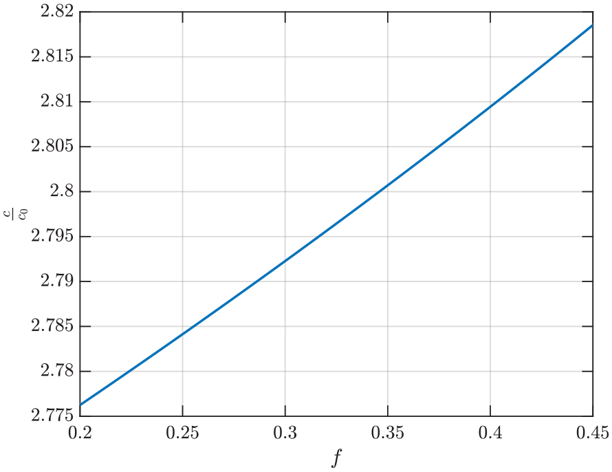
Plot showing the variation of slip zone size for a square block indenting a half-space for varying coefficients of friction.
Next we come to the issue of varying the angles of the contact defining block involved. In practice it is unlikely that two sharp corners would meet perfectly, thus meaning that it makes most sense to consider a block of differing angle indenting a half-space. Furthermore, any slip displacements will destroy the nature of the contact. The method described can tackle such problems, although they are of little practical interest. It is worth noting, however, that in the case where the contacting bodies have the same geometry so the contact interface is colinear with the wedge bisector, then no slip will occur, as by definiton only mode I stresses are present, in which case the ratio of shear to normal stress is invariant with distance from the origin.
Returning to the problem of a block indenting a half-plane, turning now to the result when we vary the angle of the indenter between
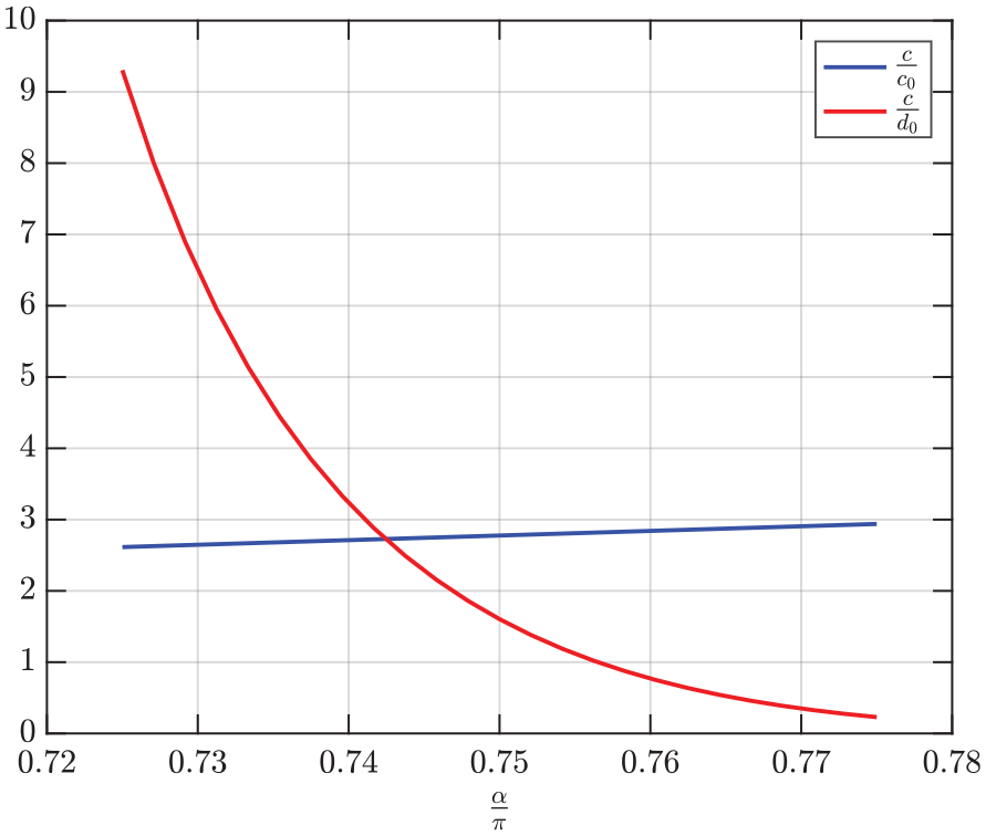
Plot showing the variation of slip zone size for block of various internal angles indenting a half-space.
The first of these bounds is that the mode
Plot showing the variation of
When the ratio
meaning that the stress ratio is given by
and is thus invariant with
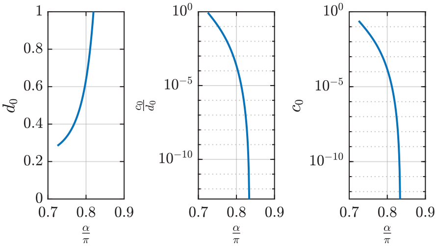
The variation of
Plot showing the variation of
Comparison of inversion methods
As we progress with the bounded-bounded quadrature, it is perhaps wise to check that the results that we get using this method are not dissimilar to those found using the singular-bounded quadrature, when supplying that method with the correct size for the slip zone. Figure 11 shows an overlay plot of the stresses and slip displacements for the two methods for a square indenter with coefficient of friction
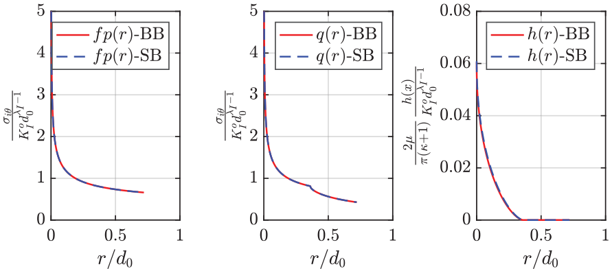
Plot showing an overlay of the stresses calculated using the bounded-bounded (red) and singular-bounded (blue, dashed) quadratures.
Discussion
These results are satisfactory and make sense on an intuitive level. However, so far several problems have been left open in this analysis. The first of these, that we will discuss is, “Why are the two conditions which previously were sufficient, now only necessary, these being the friction law and orthogonality conditions?”
In attempting to answer this question, let us consider briefly a different problem. Consider the problem of an semi-infinite incomplete contact, loaded so as to produce a zone of partial slip at the contact edge. These problems are not the same: the incomplete contact is uncoupled, that is changes in the normal traction or normal load will not affect the shear traction and vice versa. Secondly, the contact pressure is square root bounded at the contact edge. The adhered shear traction is square root singular, and we may use a distribution of dislocations to apply a corrective term to model slip.
Happily, on this occasion, a simpler dislocation kernel may be used, and Moore et al. 26 were able to find a closed form solution by inverting the integral equation. This also gives us a true size for the slip zone. However, using a dislocation formulation, we can observe the state of stress generated if the modelled slip zone size is forced to be either too small or too large.
We denote the size of the slip zone calculated by Moore et al. as
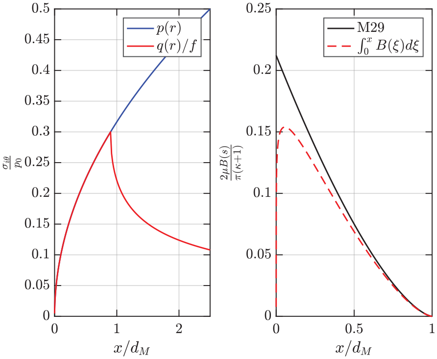
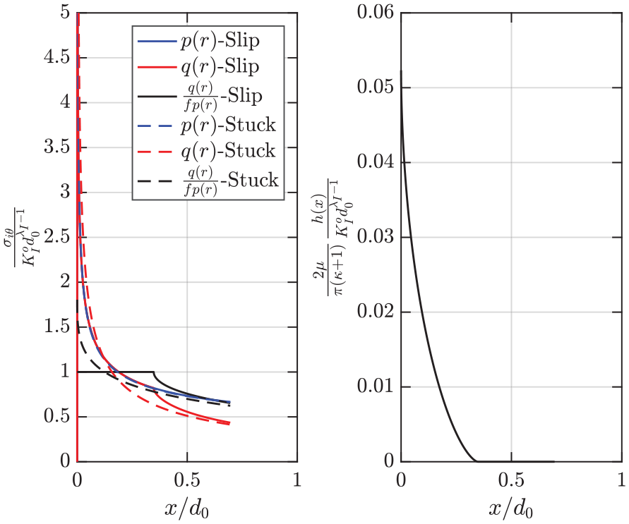
Plot showing the surface tractions (left hand plot) and slip displacement (right hand plot) for a slipping incomplete contact with a slip zone 90% of the true size.
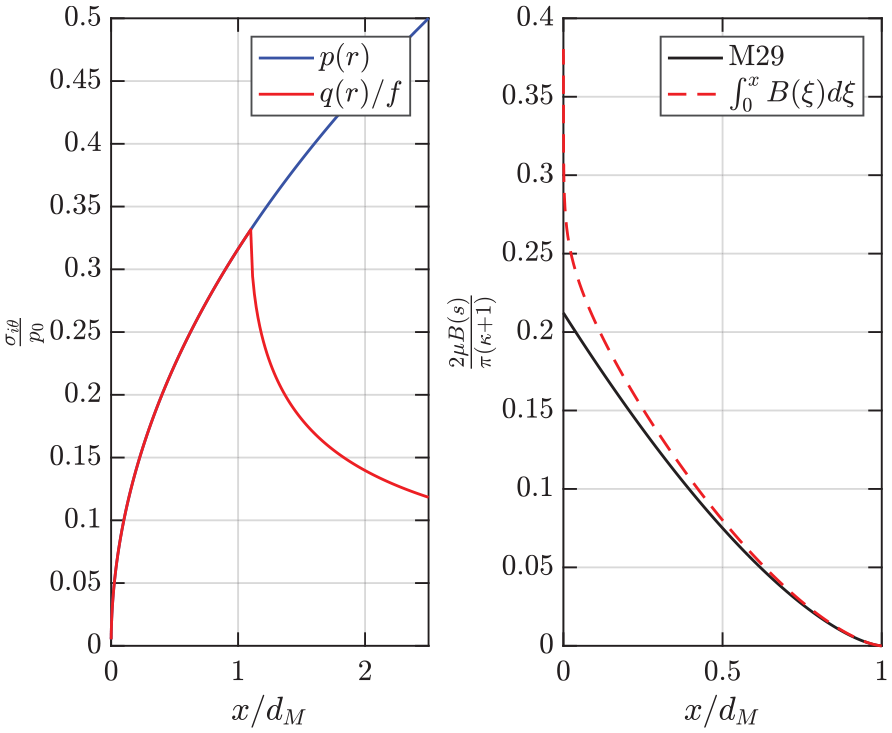
Plot showing the surface tractions (left hand plot) and slip displacement (right hand plot) for a slipping incomplete contact with a slip zone 110% of the true size.
For all the reasons previously stated, these problems are not the same, and the behaviour of the stresses is very different, most notably the corrected solution is not singular. However, it is noteworthy that the same problems arise when trying to determine slip zone size in another semi-infinite contact, using the same friction law and orthogonality conditions.
Sliding asymptote
We have already stated that the sliding solution may not be used to constrain the slip solution with any confidence as we are not able to say over what range the asymptotic representation is correct. Even once we have a solution that we are happy with this is a difficult problem, as we do not have values for the sliding stress intensity factor.
However, the sliding asymptote may be fitted to our slip traction at the edge of contact, where an accurate representation is expected. Doing this will obviously result in a very good match at the points which we use for the fit, but it is instructive nevertheless, as it gives an indication of how good an approximation the sliding asymptote is throughout the slip region.
Figure 14 shows a comparison of the tractions found using our method described above and the sliding asymptote, fitted at the edge of contact. The ratio between the two (Figure 14, dashed black line) is particularly instructive as it shows that the asymptotic approximation remains close to the calculated traction for a large portion of the slip region.
Plot showing a comparison of the slip and sliding tractions.
Slip displacements
When discussing the slip displacements calculated using the singular bounded quadrature, we stated that we are unable to exclude the possibility of a turning point in the slip displacement, but in all cases examined so far no turning point has been present. So the question may be asked, does a turning point arise, or, as expected, is no turning point present?
Figure 15 shows a normalised overlay of the slip displacements found for five different cases for the coefficient of friction (left hand plot) and for five different angles (right hand plot). It can be seen that the form of each of these is broadly similar, and none displays a turning point behaviour. This is by no means a rigorous proof, or an exhaustive examination, but it is indicative that it seems extremely unlikely that a turning point in slip displacement might be observed.
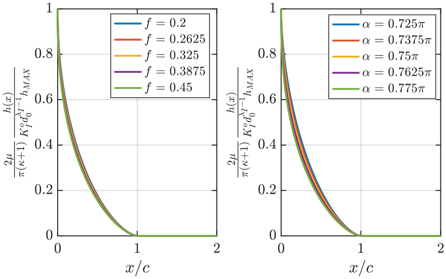
Plot showing a normalised overlay of the slip displacements for different coefficients of friction (left hand plot) and indenter angles (right hand plot).
Conclusion
In this analysis, we have determined the size of a zone of partial slip at the edge of a complete contact. We have shown how the size of this slip zone varies with changes in the coefficient of friction, and the contact angle. This includes a correction of previously published results. Furthermore, bounds have been placed on the range of validity of the asymptotic solution, and/or the existence of a slip region.
Additionally, we have discussed and explored two different numerical methods, and the reasons for choosing either method. Previous conditions used to determine the size of the slip zone have been investigated, and have proved insufficient. Alternative constraints have been explored and ruled out, although these are shown to also be true, but not enforceable as constraints. Finally, a method is arrived at using a feature of one of the numerical methods, although the choice of numerical quadratures has been shown not to affect the solution.
Footnotes
Declaration of conflicting interests
The author(s) declared no potential conflicts of interest with respect to the research, authorship, and/or publication of this article.
Funding
The author(s) disclosed receipt of the following financial support for the research, authorship, and/or publication of this article: Both authors thank Rolls-Royce plc and the EPSRC for the support under the Prosperity Partnership Grant ’Cornerstone: Mechanical Engineering Science to Enable Aero Propulsion Futures’, Grant Ref: EP/R004951/1.