Sage Journals: Discover world-class research

Abstract

Limited driving range and availability of charging infrastructures are still among the main barriers of adoption of electric vehicles (EVs) in the market. Combination of those limiting factors causes ‘range anxiety’ in EV users. While different EV battery technologies and charging infrastructures are under development, one short-term solution to reduce EV users’ range anxiety is to provide the EV user with an accurate range estimation. In this study, an EV range estimation technique is proposed that recognises the current driving pattern and then classifies it into one of the predefined clusters (driving modes). The future energy consumption per kilometre is then tuned according to the average energy consumption of each cluster. Having an updated energy consumption rate, the EV range is calculated based on the battery state-of-charge. Different features are considered for driving pattern clustering where ‘average speed’ and ‘average power’ were identified as the best choices for this application. The effectiveness of the proposed EV range estimator is validated using real driving data that gives an average error of 9% in EV energy consumption estimation ahead.

Keywords

Electric vehicle range estimation driving pattern recognition clustering energy consumption

Introduction

Electric vehicle (EV) technologies are growing quickly mainly because of their zero local emissions (i.e. direct tailpipe emissions). However, limited driving range, long charging time and in some areas, limited number of charging infrastructures are still the main barriers to the adoption of EVs in the market.^1,2 The combination of those limiting factors cause a phenomenon called ‘range anxiety’,^3–5 which refers to the driver’s fear of running out of energy before arriving the destination. Although range anxiety could be alleviated by increasing the battery pack’s capacity, increasing the allowable charging power, and building more charging stations, those solutions are quite expensive and do not directly improve the driver’s confidence on the remaining driving range (RDR). EV drivers often reserve a buffer of around 20% of the battery capacity to avoid running out of energy on the journey.⁶ To make the most use of the limited battery capacity, providing EV users with an accurate RDR estimation is same important as increasing the maximum range.⁷ Therefore, while different EV battery technologies and charging infrastructures are under development, a short-term solution to alleviate EV users’ range anxiety, is to provide an actuate RDR estimation.^8–12

EV RDR estimation is a very challenging task due to the uncertainties in future driving condition (i.e. driving pattern, traffic condition), environmental factors (i.e. ambient temperature, wind, rain), and battery state (i.e. nonlinearity, ageing), etc. There are a number of techniques for RDR estimation in the literature, which are classified into two main categories: (i) history-based and (ii) model-based estimation techniques.^13–19

The history-based methods assume that the immediate future energy consumption is same as the very recent energy consumption. In other words, the remaining range prediction relies on past energy consumption data.^20–23 Because of its less complexity, this technique is commonly used in the existing RDR estimators on commercial vehicles. However, the accuracy of this technique suffers from the frequent fluctuations in energy consumption that happen in a real driving scenario. This consequently causes fluctuations in RDR estimations shown on dashboard that can potentially make it unreliable for the EV user. To tackle this issue, EV manufacturers have proposed some solutions. Tesla Model S provides either instant range or average RDR estimation.²⁴ Instant range utilizes the latest few data points to calculate range while the average range utilizes average energy consumed over the last 10, 25 or 50 km of the journey. When navigated to a destination, Tesla Model S can also predict energy usage based on driving style (predicted speed, etc.) and environmental factors (elevations, temperature, etc.). The RDR of Nissan Leaf is calculated based on the historical actual power consumption average.²⁵ The Renault Zoe estimates RDR using the average energy consumption data over the last 200 km.²⁶

On the other hand, model-based methods estimate the remaining range in a more complicated way by using adaptive algorithms or machine learning techniques to predict future speed profile, future energy consumption and remaining battery energy^27,28 as discussed in the following.

Markov model is utilised in a study by Oliva et al.^29,30 to predict the driving speed profile in the near future. Various sources of uncertainty such as driving pattern and measurement noise have been considered in those studies. Their RDR estimation algorithm consists of two steps. Firstly, the battery state is estimated by a particle filter²⁹ or Kalman filter.³⁰ Secondly, the future driving profile is predicted using Markov chain. Then according to the distribution of the propagated particles, the RDR has been estimated as a probability distribution. In another study by Pan et al.,³¹ Markov chain together with artificial neural network (ANN), is utilised to estimate the RDR. The estimation process is divided into offline and online stages. At the online stage, the real-time driving condition is recognised and then classified into one of the four predefined clusters, after which the Markov chain and ANN are used to predict the future driving conditions based on the driving pattern. The average energy consumption of each cluster is calculated at the offline stage. Once the current driving condition is recognised, the corresponding energy consumption is identified and the RDR is computed.

Liu et al.³² introduced a method called RDR Information Fusion (RDRIF). The RDR is estimated by the fusion of both the calculated and cumulated range. The calculated range is obtained from the data of the present battery state and vehicle energy consumption, while the cumulated range is the cumulation of the real travelled distance. The experiment results show that after the initial stage the estimator error is less than $\pm$ 5%. Adnane et al.³³ proposed a new driving mode predictor (DMP) using machine learning models, which are obtained from EV’s speed history. The DMP is then used in energy management system of a dual-source EV. In another study, Sonalikar et al.³⁴ implemented a simplified approach to calculate the driving range using Kalman filter and real-time vehicle data. In that technique, the initial error might be large however, it could be reduced by using static or history energy consumption at the beginning of the estimation. Assuming that in the next decades there will be more vehicles connecting to a server in the back-end, Grubwinkler et al.³⁵ used a cloud-based method to gather speed information from diverse vehicles and drivers. Then the estimation model predicts the energy consumption along a given road by utilising the previously obtained data. The energy consumption value is then used for RDR calculation.

In conclusion, model-based methods are more accurate, but they need lots of data as input and higher computational effort that might not be feasible to be implemented in a passenger car. On the other hand, while less accurate, history-based range estimators are easy to be implemented in the vehicle for real-time application, though they are not accurate enough as discussed earlier.

In general, the EV RDR depends on two factors: (i) available energy in the battery pack, and (ii) energy consumption as a function of the conditions in which the vehicle is operating. Information about the first factor (i.e. battery state of charge) is available in all commercial EVs. However, the second factor is very difficult to be predicted. According to the literature, driving pattern has a significant impact on the energy consumption.³⁶ Driving pattern can be presented in different ways where a common form is the speed profile verse time. There are different methods in the literature, which are developed for driving pattern information analysis and prediction. These methods can be classified into two main categories, namely driving pattern prediction and driving pattern recognition.^37,38 In the prediction category, the traffic and geographic information provided by GPS or digital maps is used to predict vehicle’s speed, elevation and so on. Instead of predicting future driving patterns, the driving pattern recognition methods extract features of the past driving pattern to recognise the existing driving mode (no future prediction) and assume that the driving pattern will not change in a very short time horizon. In literature,³⁹ field tests were conducted to gather real driving data, and then driving data segmentation and feature extraction have been performed to investigate the influence of the features on vehicle energy consumption using computer simulation. Feng et al.⁴⁰ studied a supervised driving pattern recognition method, based on which, each driving pattern is represented by a feature vector, which is formed by a set of parameters sensitive to the driving pattern. The online driving pattern recognition can be realised by computing feature vectors and then cluster the current driving pattern to one of the driving modes in the reference database. There are also other studies in the literature in which the concept of driving pattern (also called driving mode) recognition is utilised for energy management in hybrid vehicles.^41–44

This study is focused on creating a multi-mode EV range estimator based on driving pattern recognition (DPR). Although the concept of DPR already exist in the literature, the application of such technique for EV RDR estimation is done here for the first time. The proposed RDR estimation technique aims to fill the gap between the history-based techniques (with more simplicity) and the model-based techniques (with more accuracy) by proposing a proper trade-off between accuracy and simplicity for real-time applications. In other words, the proposed technique is an advanced history-based method, which is intelligent enough to distinguish between different driving patterns.

Structure of this paper is as follows. The next section discusses the RDR estimation strategy. Then, driving data segmentation and energy consumption of each cluster are discussed. ‘Driving pattern clustering’ section discusses the proposed driving pattern clustering technique using different features. RDR estimation and the validation results are investigated in the penultimate section. The final section includes the conclusions.

Range estimation strategy

A history-based method is chosen for range estimation in this study which is model-free and without the need for high computational effort. Therefore, it is potentially applicable for real-time applications. As mentioned in the Introduction section, the EV RDR depends on (i) battery pack’s available energy and (ii) energy consumption. Since the available energy on board can be obtained from the battery management system (BMS), this paper only studies the second component, that is energy consumption.

Based on the fact that driving pattern rarely changes in a very short time interval, it is reasonable to assume that the driving pattern over the next few seconds is very similar to that in the short history of motion. The flow chart of the proposed RDR estimation technique is shown in Figure 1. It consists of offline and online stages. The proposed strategy is designed such that it recognises the current driving pattern (based on a short history of motion) and then, the near future driving pattern is assumed to be same as the current one. The online recognition process is repeated frequently to avoid use of old information while driving. The near future average energy consumption (Wh/km) is then estimated based on the identified cluster (here each cluster means a driving mode). The average energy consumption of each cluster is calculated offline, which is explained in more detail in ‘Driving data segmentation and energy consumption calculation’ section. Having the battery remaining energy information, the RDR (km) is calculated by dividing the available battery pack energy (Wh) by the future average energy consumption value (Wh/km). When the driving pattern changes, the average energy consumption value is also updated to the value corresponding to the new recognised driving mode.

Figure 1.

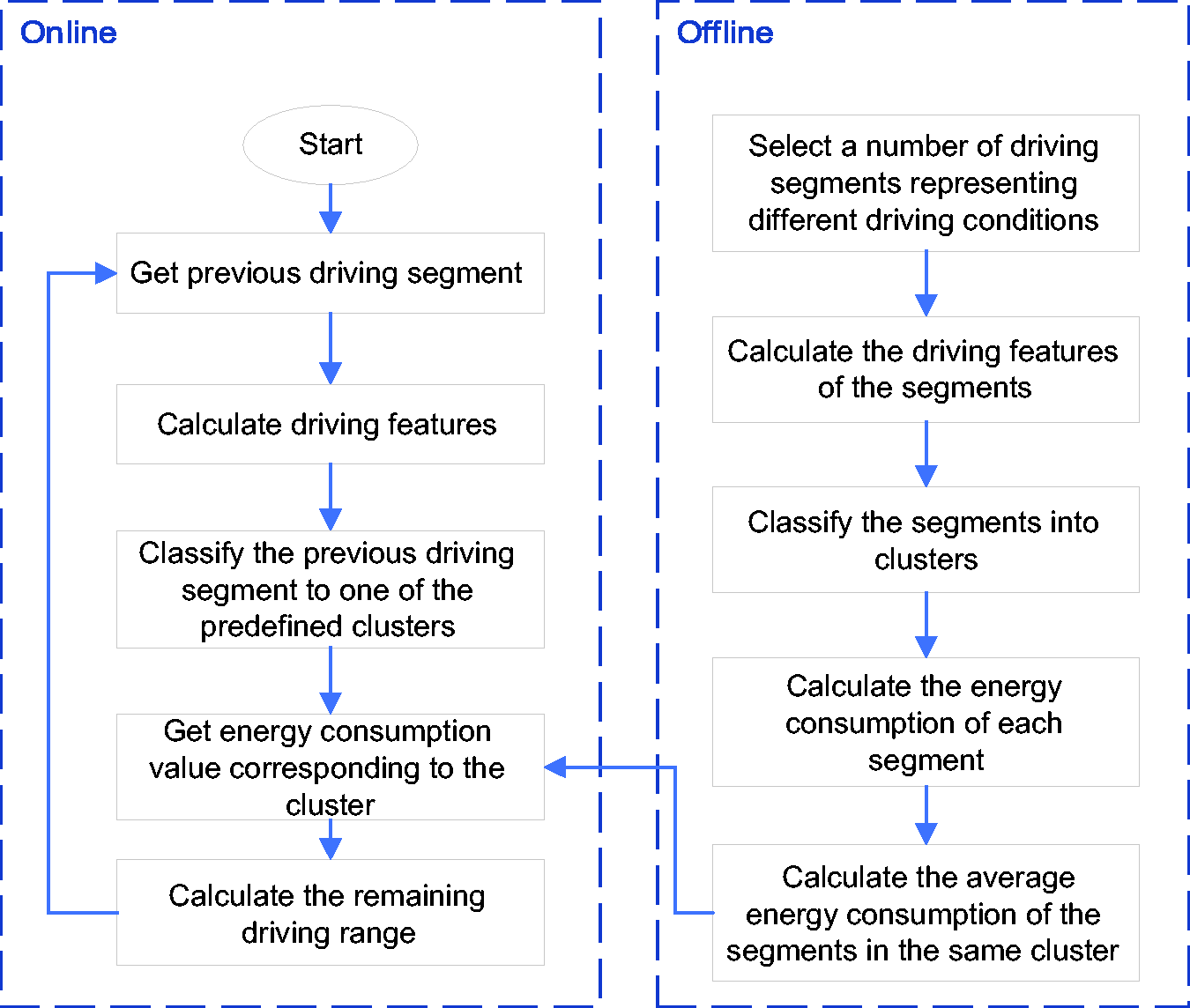
Proposed RDR estimation strategy.

Based on this definition, the segments in same cluster are assumed to have similar energy consumption per kilometre, although it is known that there is a variance between the energy consumption of each individual segment and the cluster’s average energy consumption. It is possible to decrease this deviation by defining more clusters however, the drawback of that solution is to have more transitions between clusters in real-time, which can be another source of error. So, a proper trade-off between the number of clusters and overall performance of the system is necessary. Different number of clusters are investigated in this study as discussed in the following sections.

According to the proposed RDR estimation strategy, the RDR could be calculated through equation (1):

RDR = \frac{{R E}_{battery}}{E_{consumption}}

(1)

{R E}_{battery} = SOC * C

(2)

where

RDR

is the remaining driving range (km),

{R E}_{battery}

is the remaining energy (Wh) in the EV battery,

E_{consumption}

is the average energy consumption value corresponding to the current driving mode (Wh/km),

SOC

is the battery state of charge (%), and

C

is the energy capacity of the EV battery pack (Wh).

Driving data segmentation and energy consumption calculation

EV energy consumption model

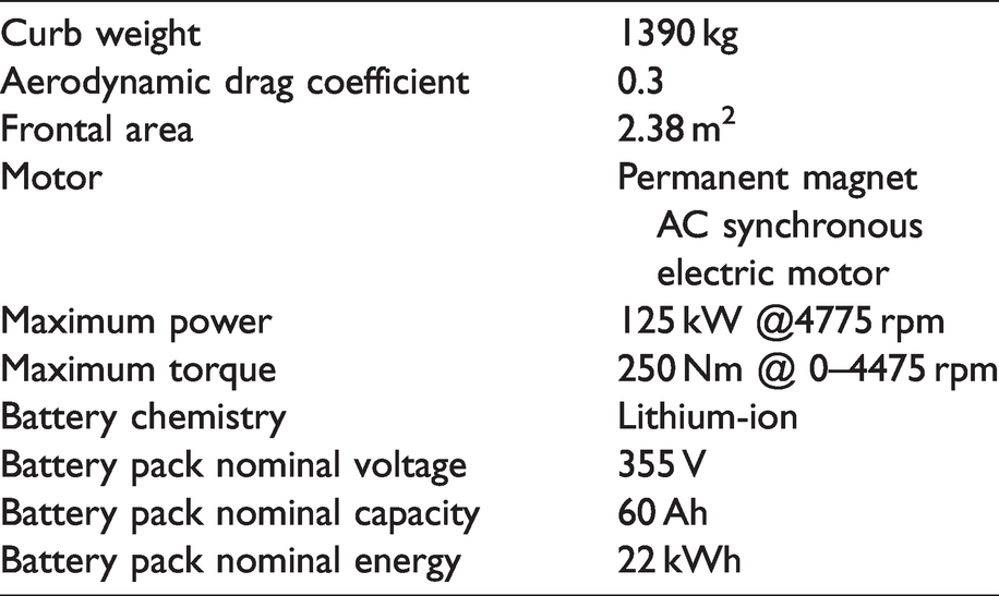
An accurate EV model is the prerequisite to calculate the energy consumption. The EV that is considered in this study, is BMW i3 with specifications presented in Table 1. The EV model which is used in this study, has been presented in full details in literature.⁴⁷ It consists of driver model, brake system, power electronics and electric motor, battery model, transmission system, auxiliary loads, and longitudinal vehicle dynamics. As discussed in literature,⁴⁷ the model has been validated against experimental test data, which has demonstrated a satisfactory level of accuracy in terms of energy consumption calculation.

Table 1.

BMW i3 specifications.^45,46

Curb weight	1390 kg
Aerodynamic drag coefficient	0.3
Frontal area	2.38 m²
Motor	Permanent magnet AC synchronous electric motor
Maximum power	125 kW @4775 rpm
Maximum torque	250 Nm @ 0–4475 rpm
Battery chemistry	Lithium-ion
Battery pack nominal voltage	355 V
Battery pack nominal capacity	60 Ah
Battery pack nominal energy	22 kWh

It should be noted that the EV model is only used for offline energy consumption analysis. As mentioned in the Introduction section, this study aims to combine the history of vehicle motion in real-time with the offline model-based energy consumption analysis to improve EV range estimation accuracy. Driving data segmentation

In order to analyse a continuous signal of driving data measured in real-time, one common technique is to divide it into small segments. There are two methods in the literature to partition a measured speed profile: segment and micro-trip.^48,49 A driving segment refers to a section of the speed profile, which is recorded in a certain period of time (a predefined length) as shown in Figure 2 (the segment length is set as 120 s in this example). On the other hand, a micro-trip is defined as a section of the speed profile but from one stop to another stop, as shown in Figure 3. The micro-trip segmentation technique is more useful for other applications such as driving cycle development as discussed in literature.⁴⁸ Therefore, in this study, the time segmentation method is selected to partition the speed profile, as it has a distinct length, which makes it easier to be implemented in real-time.

Figure 2.

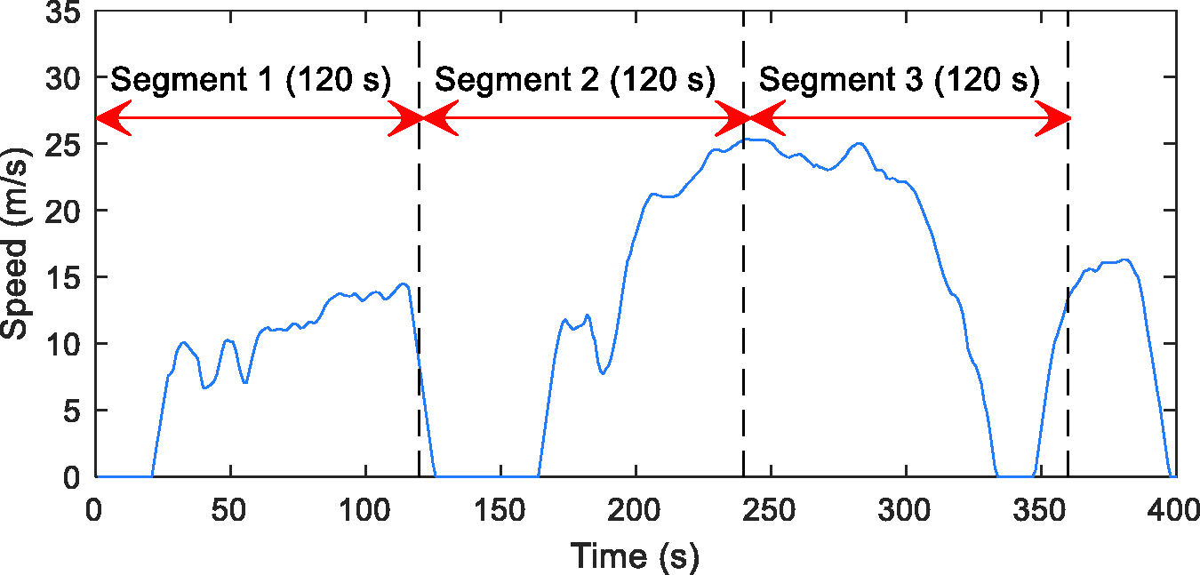
Driving segments.

Figure 3.

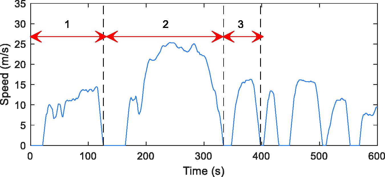
Driving micro-trips.

Sample data for offline energy consumption calculation

A range of standard driving cycles is utilised to generate a set of data that includes samples of driving segments. The data set includes driving in different types of road, different traffic conditions (congested, urban, suburban, and highway), and different driving behaviours. The driving data set is generated by combining the following 11 drive cycles as shown in Figure 4: UDDS, US06, SC03, NYCC, HWFET, FTP, WLTP Class 3, Artemis Road, Artemis Urban, Artemis Motorway 130, and Artemis Motorway 150. In the next section, the driving data set is divided into a number of segments for energy consumption analysis.

Figure 4.

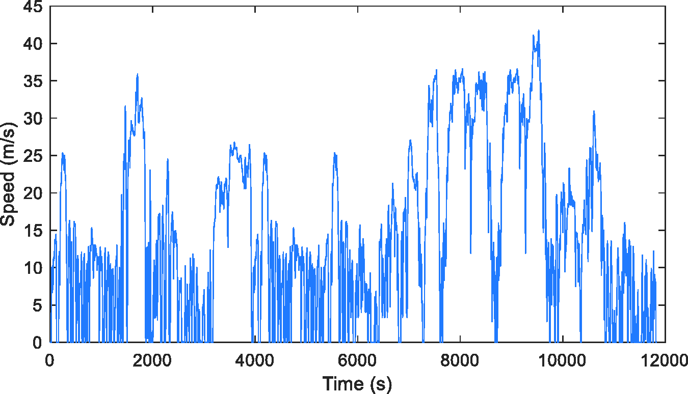
Combined speed profile based on different drive cycles.

It should be noted that the data set generated in this section using the standard drive cycles is not used for RDR estimation validation. For validation purpose, a separate set of data is used, which is collected by performing field measurements as explained in the following sections.

Energy consumption calculation

In a real application, the battery current and voltage signals are available from BMS control board, so the electrical power coming out of the battery can be easily calculated. Then the energy consumed at each driving segment can be obtained by integrating the power signal. In the EV model also the same approach is used where the energy coming out of the battery is computed by integrating the product of the battery pack current and voltage:

E = \frac{1}{3600} \int U * Idt

(3)

where

E

is the energy consumed in the segment (Wh),

U

is battery pack voltage (V),

I

is battery pack current (A).

The combined speed profile (shown in Figure 4) is used as the input of the simulation model. The EV model is simulated over the whole speed profile to obtain the energy consumption value corresponding to each driving segment as presented in below:

E_{seg} = E_{seg_end} - E_{seg_start}

(4)

where

E_{seg}

is the battery pack’s energy consumed in a segment (Wh), and

E_{seg_end}

and

E_{seg_start}

are the values of energy consumption recorded at the end and start of the segment respectively (Wh). For better understanding of equation (4), its parameters are shown in Figure 5.

Figure 5.

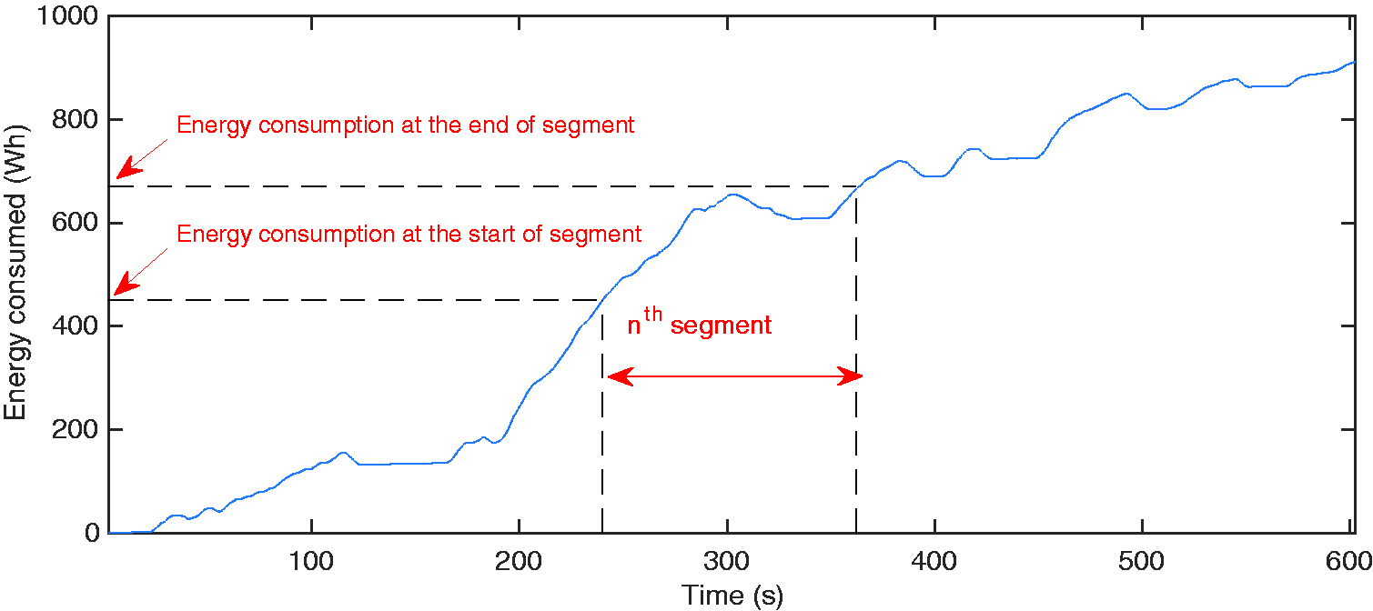
Energy consumption calculation during a single segment.

The value of distance travelled is also recorded in form of a time-series to calculate the average speed of each segment. The distance travelled in one segment can be obtained using the following equation:

d_{seg} = d_{seg_end} - d_{seg_start}

(5)

where

d_{seg}

is the distance travelled during a segment (km), and

d_{seg_end}

and

d_{s e g_start}

are the values of distance travelled recorded at the end and start of the segment respectively (km) as shown in Figure 6.

Figure 6.

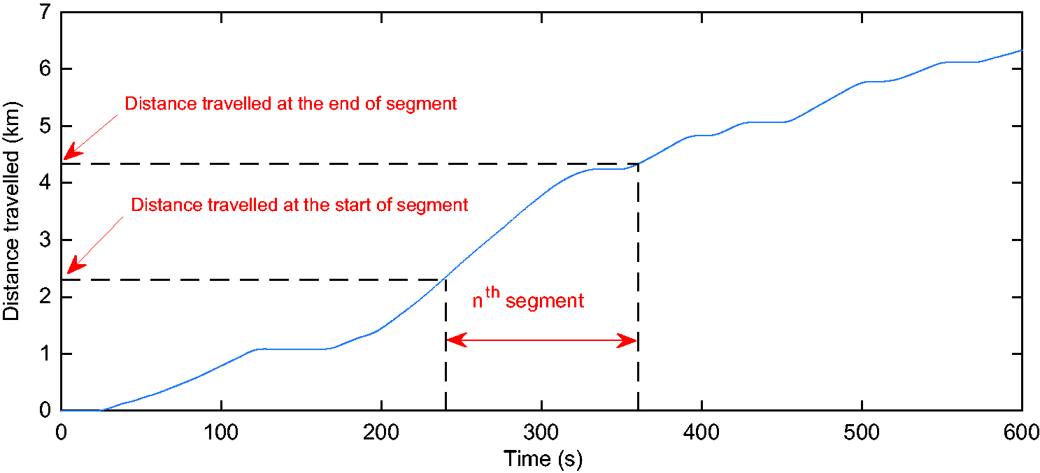
Distance travelled in a segment.

The average speed of each segment can then be calculated as follows:

v_{avg} = \frac{d_{seg}}{t_{seg}} * 1000

(6)

where

v_{avg}

is the average speed of the segment (m/s),

d_{seg}

is the distance travelled in the segment (km), and

t_{seg}

is the segment’s time length (s).

The energy consumption per unit of distance can then be calculated using equation (7):

E_{con_seg} = \frac{E_{seg}}{d_{seg}}

(7)

where

E_{con_seg}

is the energy consumption per unit of distance (Wh/km),

E_{seg}

is the energy consumed during a segment (Wh), and

d_{seg}

is the distance travelled over that segment (km).

Finally, the average energy consumption of all the segments in the same cluster is calculated using equation (8):

E_{con_cluster} = \frac{1}{n} \sum_{i}^{n} {E_{con_seg}}_{i}

(8)

where

E_{con_cluster}

is the energy consumption per unit of distance for a cluster (Wh/km),

n

is the number of the segments belong to that cluster, and

{E_{con_seg}}_{i}

is the energy consumption per unit of distance for the

i^{th}

segment of that cluster (Wh/km).

Driving pattern clustering

In order to recognise driving patterns in real-time, a set of parameters (features) need to be defined to characterise them first. As mentioned in the Introduction section, different driving features have been proposed in the literature to analyse driving patterns. For real-time applications, the driving features should be as simple as possible to reduce computational effort. For that reason, a single feature or very limited number of features are desirable. According to the literature, EV energy consumption (and consequently the EV range) is very sensitive to features such as ‘average speed’ and ‘average power’.³⁹ In the following sections, those two features are investigated individually and then together in order to characterise the driving patterns.

Driving pattern clustering using average speed

In this section, the driving segments are clustered into different number of groups based on their average speed. As driving data segmentation was discussed in ‘Driving data segmentation’ section, different values of segment length are considered. According to the literature, both the number of clusters and the length of the segments could influence the clustering performance.⁴⁰ Therefore, different combinations of cluster numbers and segment lengths are investigated. For that purpose, the speed profile is partitioned into 60, 120, 180, 240, 300, 360-sec length segments respectively. On the other hand, to investigate the impact of the number of clusters, the driving segments are clustered into 3, 4, and 5 groups.

In the data set presented in ‘Sample data for offline energy consumption calculation’ section, the maximum average speed is around 40 m/s, so the cluster boundaries are divided equally from 0 to 40 m/s:

In first case, the driving segments are clustered into 3 groups as follows:

Cluster 1: $s_{ave} <$ 13 m/s

Cluster 2: 13 $\leq s_{ave} <$ 26 m/s

Cluster 3: $s_{ave} \geq$ 26 m/s

In the second case, the driving segments are clustered into four groups:

Cluster 1: $s_{ave} <$ 10 m/s

Cluster 2: 10 $\leq s_{ave} <$ 20 m/s

Cluster 3: 20 $\leq s_{ave} <$ 30 m/s

Cluster 4: $s_{ave} \geq$ 30 m/s

And in the third case, the driving segments are clustered into five groups:

Cluster 1: $s_{ave} <$ 8 m/s

Cluster 2: 8 $\leq s_{ave} <$ 16 m/s

Cluster 3: 16 $\leq s_{ave} <$ 24 m/s

Cluster 4: 24 $\leq s_{ave} <$ 30 m/s

Cluster 5: $s_{ave} \geq$ 30 m/s

Where: $s_{ave}$ Is the average speed of the segment.

As an example, Figure 7 shows the average speed of all the segments in the case of three clusters and segment length of 60 seconds, which includes 197 segments in total.

Figure 7.

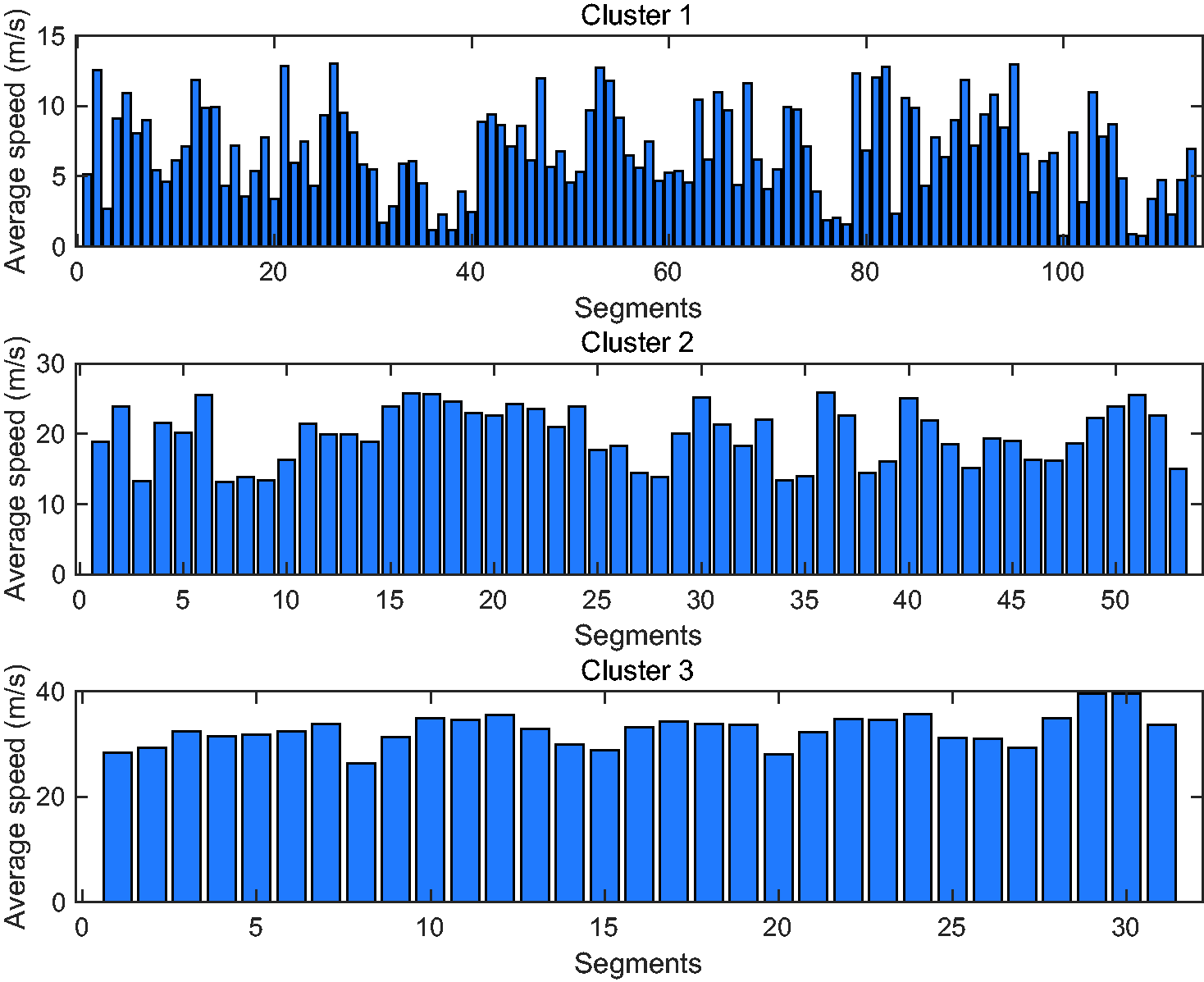
Average speed of segments in different clusters.

It should be noted that the simple clustering technique that is used here is selected intentionally because the data set was limited (as discussed in ‘Sample data for offline energy consumption calculation’ section). In real implementation of this technique (assuming a large data set), the speed boundaries can be determined using other clustering techniques based on the data rather than manually. For example, k-means clustering technique is used in literature⁵⁰ for real driving data clustering.

Driving pattern clustering based on average power

In this section, ‘average power’ demand during each segment is used as a feature for clustering of the driving segments. The power signal can potentially be better than the speed signal because it also includes the effect of road gradient, weight variations (e.g. Due to more passengers), and other factors that are not included in the speed profile. The battery output current and voltage are used to calculate the battery power. A similar procedure of segmentation, feature extraction and clustering is applicable for the power signal too.

In the simulation model, the battery power signal is recorded in form of a time-series. So the average battery power of each segment can be calculated using equation (9):

P_{avg} = \frac{1}{n} \sum_{i}^{n} P_{i}

(9)

Where

P_{avg}

Is the average power demand of the segment (kw),

n

is the number of the power signal data points, and

P_{i}

Is the

i^{Th}

Power signal value (kw).

To investigate the impact of segments’ length, same analysis is repeated for five different segment lengths, which includes 120, 180, 240, 300, and 360 seconds. For the data set introduced in ‘Sample data for offline energy consumption calculation’ section, the maximum average power is around 30 kw, so the clusters boundaries are set equally from 0 to 30 kw. Three different cluster numbers (3, 4, and 5) are defined as follows:

In the first case, three cluster boundaries are set as follows:

Cluster 1: $P_{avg} <$ 10 kw

Cluster 2: 10 kw $\leq P_{avg} <$ 20 kw

Cluster 3: $P_{avg} \geq$ 20 kw

In the second case, four clusters are defined:

Cluster 1: $P_{avg} <$ 7 kw

Cluster 2: 7 kw $\leq P_{avg} <$ 14 kw

Cluster 3: 14 kw $\leq P_{avg} <$ 21 kw

Cluster 4: $P_{avg} \geq$ 21 kw

And in the third case, five clusters are considered:

Cluster 1: $P_{avg} <$ 5 kw

Cluster 2: 5 kw $\leq P_{avg} <$ 10 kw

Cluster 3: 10 kw $\leq P_{avg} <$ 15 kw

Cluster 4: 15 kw $\leq P_{avg} <$ 20 kw

Cluster 5: $P_{avg} \geq$ 20 kw

Where $P_{avg}$ Is the average power of the segment (kw).

Taking the case of 60-second segments in three clusters as an example, Figure 8 shows the average power of segments for each cluster.

Figure 8.

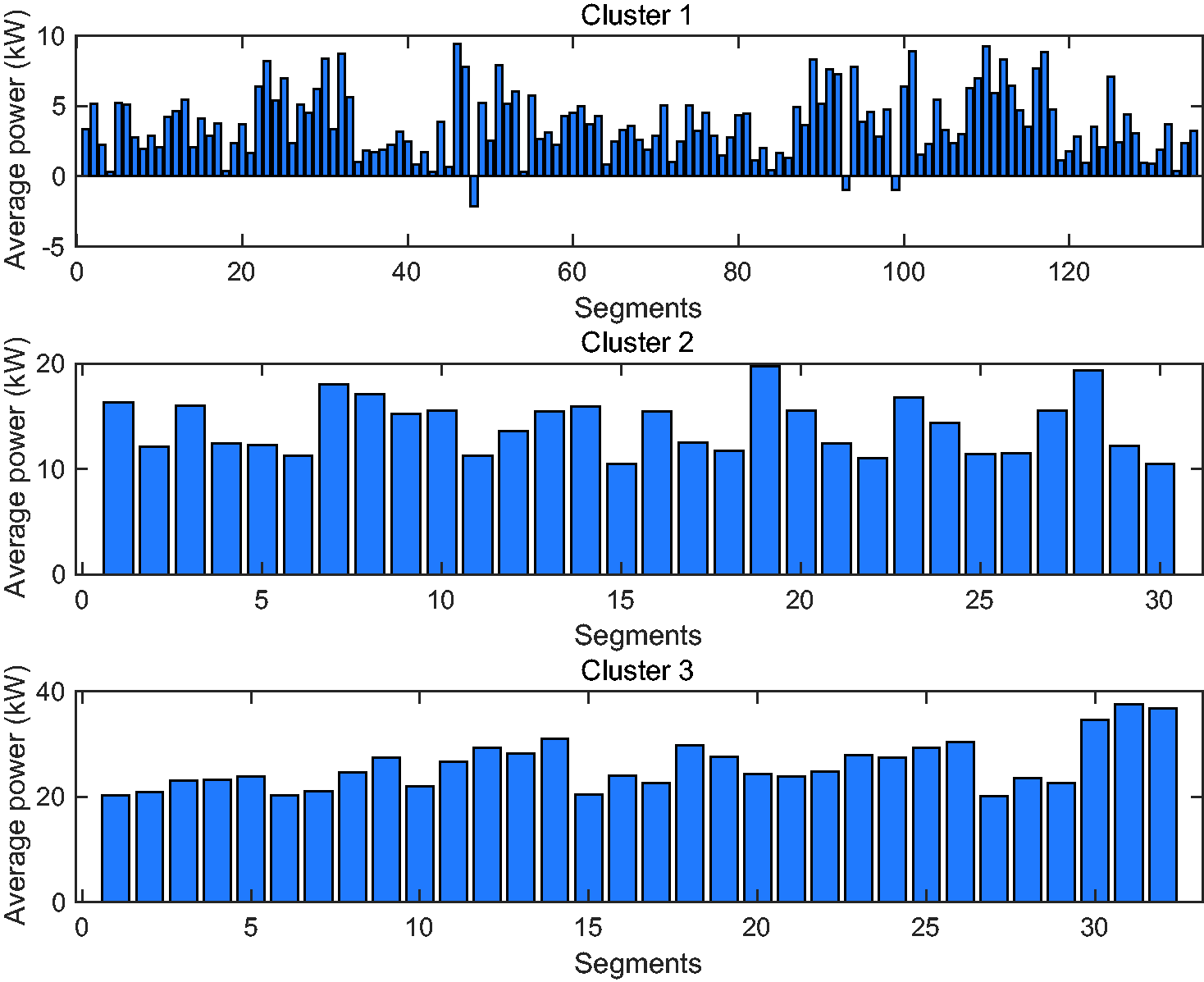
Average power of segments in different clusters.

Driving pattern clustering based on average speed and average power

In this section, both features of average speed and average power are used at the same time to classify the driving segments. In order to keep the total number of clusters at a low level (i.e. For real-time application), two regions are considered for each feature. For high-speed driving patterns, the average power is normally above 10 kw, while it is below that threshold for low-speed driving patterns. So that value is used as a reference for defining a division boundary. It should be noted that the value of power threshold is obtained for the vehicle model, which is used in this study, and a tuning process is necessary when switching to another vehicle. In terms of average speed boundary, it is assumed that driving patterns with an average speed below 10 m/s are low-speed while above 10 m/s is considered as mild- or high-speed driving pattern. Again, it should be noted that the boundaries are subject to change when vehicle specifications alter. The proposed method in this study is flexible in terms of working with a different set of clustering boundaries. The set of numbers which are selected in the simulations here, are just used to show the concept for an example vehicle.

Therefore, the segments are classified into four clusters as follows:

Cluster 1: $s_{avg} <$ 10 m/s, $P_{avg} <$ 10 kw

Cluster 2: $s_{avg} \geq$ 10 m/s, $P_{avg} <$ 10 kw

Cluster 3: $s_{avg} <$ 10 m/s, $P_{avg} \geq$ 10 kw

Cluster 4: $s_{avg} \geq$ 10 m/s, $P_{avg} \geq$ 10 kw

Where $s_{avg}$ Is the average speed (m/s), and $P_{avg}$ Is the average power (kw).

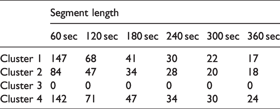
The combined standard drive cycles data set is partitioned into 60-, 120-, 180-, 240-, 300- and 360-sec segment lengths. Then in each case, the segments are classified into four clusters according to their average speed and average power. Table 2 shows the number of segments in each cluster for different segment lengths. It is found that all the segments are actually separated into only three clusters regardless of the segment’s length, as there is no segment in Cluster 3. This result is favourable because fewer clusters mean fewer changes in driving patterns, thus less fluctuation in estimated RDR. Actually, Cluster 3 includes segments with high power demand at low speed, which is not common in a real driving scenario. A good example of that is driving a sharp uphill slowly, that does not exist in our data set. For that reason, Cluster 3 is eliminated from the analysis in this study. Thus Cluster 4 becomes the third cluster, and hereinafter it is referred as ‘Cluster 3’.

Table 2.

Number of segments in each cluster.

	Segment length
	60 sec	120 sec	180 sec	240 sec	300 sec	360 sec
Cluster 1	147	68	41	30	22	17
Cluster 2	84	47	34	28	20	18
Cluster 3	0	0	0	0	0	0
Cluster 4	142	71	47	34	30	24

RDR estimation and validation

The proposed RDR estimator is validated in this section using real driving data. The speed profiles used in ‘Sample data for offline energy consumption calculation’ section are standard driving cycles, which cannot represent the real driving features. In this section, the average relative error was firstly defined to describe the accuracy of the estimator, then the real driving tests were performed on a typical EV, after which the results were compared and analysed.

Validation approach

Average relative error

At the first step to validate the effectiveness of the proposed driving segment clustering method, a relative error is defined as the difference between the energy consumption of a segment and the average energy consumption of the cluster that the segment belongs to it:

e = \frac{|E_{con_cluster} - E_{con_seg}|}{E_{con_seg}} * 100 %

(10)

where

e

is the relative error (%),

E_{con_cluster}

is the average energy consumption of the cluster (Wh/km), and

E_{con_seg}

is the energy consumption of the segment (Wh/km).

The average relative error of all the segments in the data set is considered to describe the effectiveness of the clustering method, which is obtained as follows:

e_{avg} = \frac{1}{n} \sum_{i}^{n} e_{i}

(11)

where

e_{avg}

is the average relative error (%),

e_{i}

is the relative error of the

i^{t h}

segment (%), and

n

is the number of segments.

Real driving speed profiles

At the second step of the validation process, a new real driving data set is collected by driving an EV on the road. For that purpose, because of the availability of Nissan Leaf EV, that car was used in the experiments. Although the energy consumption of BMW i3 is different from that of Nissan Leaf, here the aim of the experiments is not to model the vehicle but to extract real speed profiles for a typical EV. Similar to the standard drive cycles, which can be used for simulation of different types of vehicles, the collected real velocity profiles are assumed to be useable in the same way. More details about the test vehicle can be found in literature,⁵¹ however, it should be clarified that all the simulation models and results in this study are obtained for BMW i3.

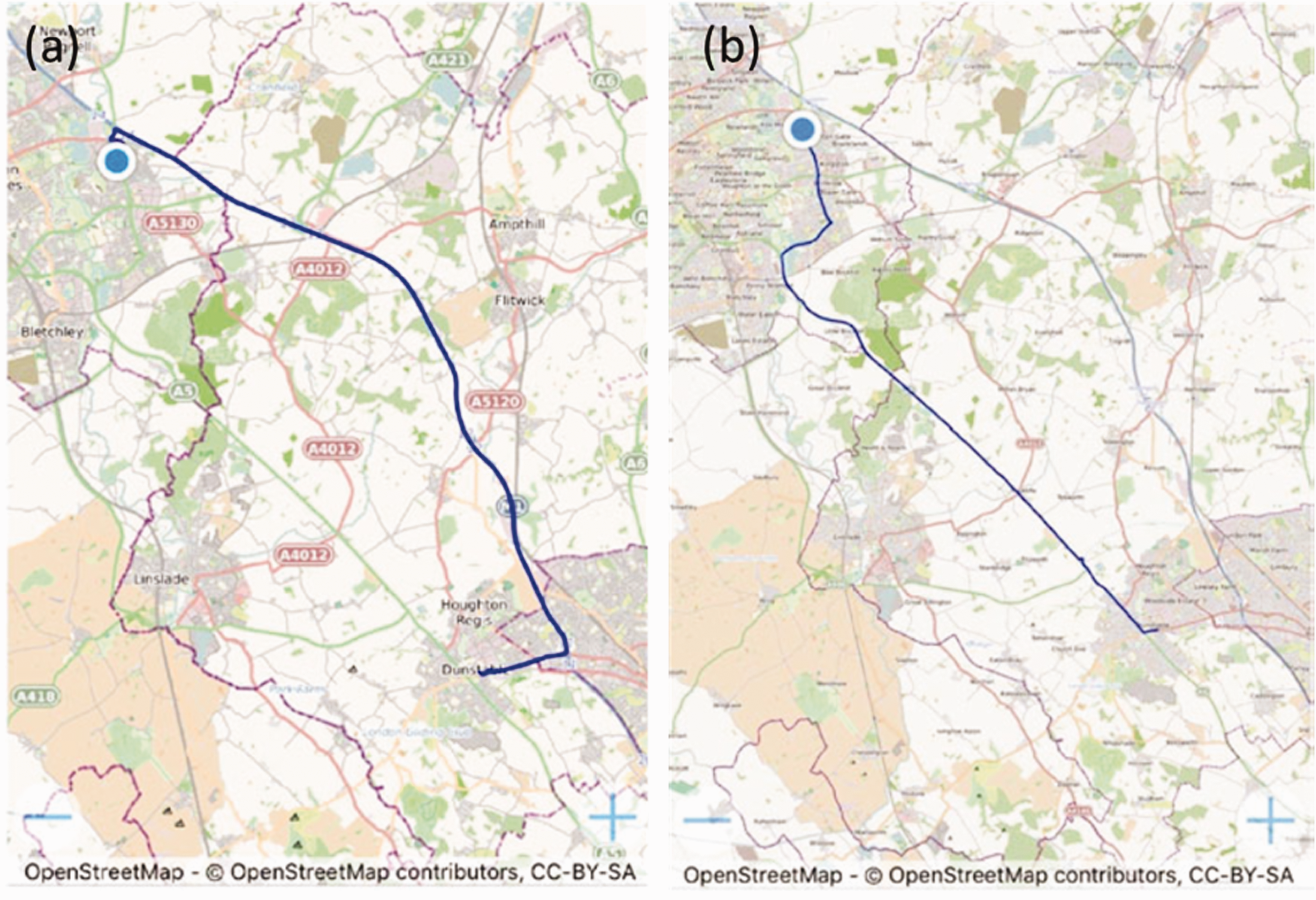
To include a range of different types of road, such as motorway, rural, and urban road, two routes were selected as follows:

Route A, from Dunstable to Milton Keynes: it mainly consists of high-speed driving in a motorway; the length of this route is about 31 km as shown in Figure 9(a).

Figure 9.

Experimental test routes: (a) test route A, which is from Dunstable to Milton Keynes, (b) test route B, which is from Milton Keynes to Dunstable.

Route B, from Milton Keynes to Dunstable: this route is completely different from the other route from Dunstable to Milton Keynes. It mostly contains extra-urban and urban roads; the length of that road is about 26 km as shown in Figure 9(b).

A total of six tests were conducted, numbered as Test 1 to Test 6, which are plotted in Figure 10. Each of the journeys is partitioned into segments with different segment length, then the average speed and average power of each segment are calculated. Thereafter, the driving segments of each test are classified into clusters as discussed in ‘Driving pattern clustering’ section.

Figure 10.

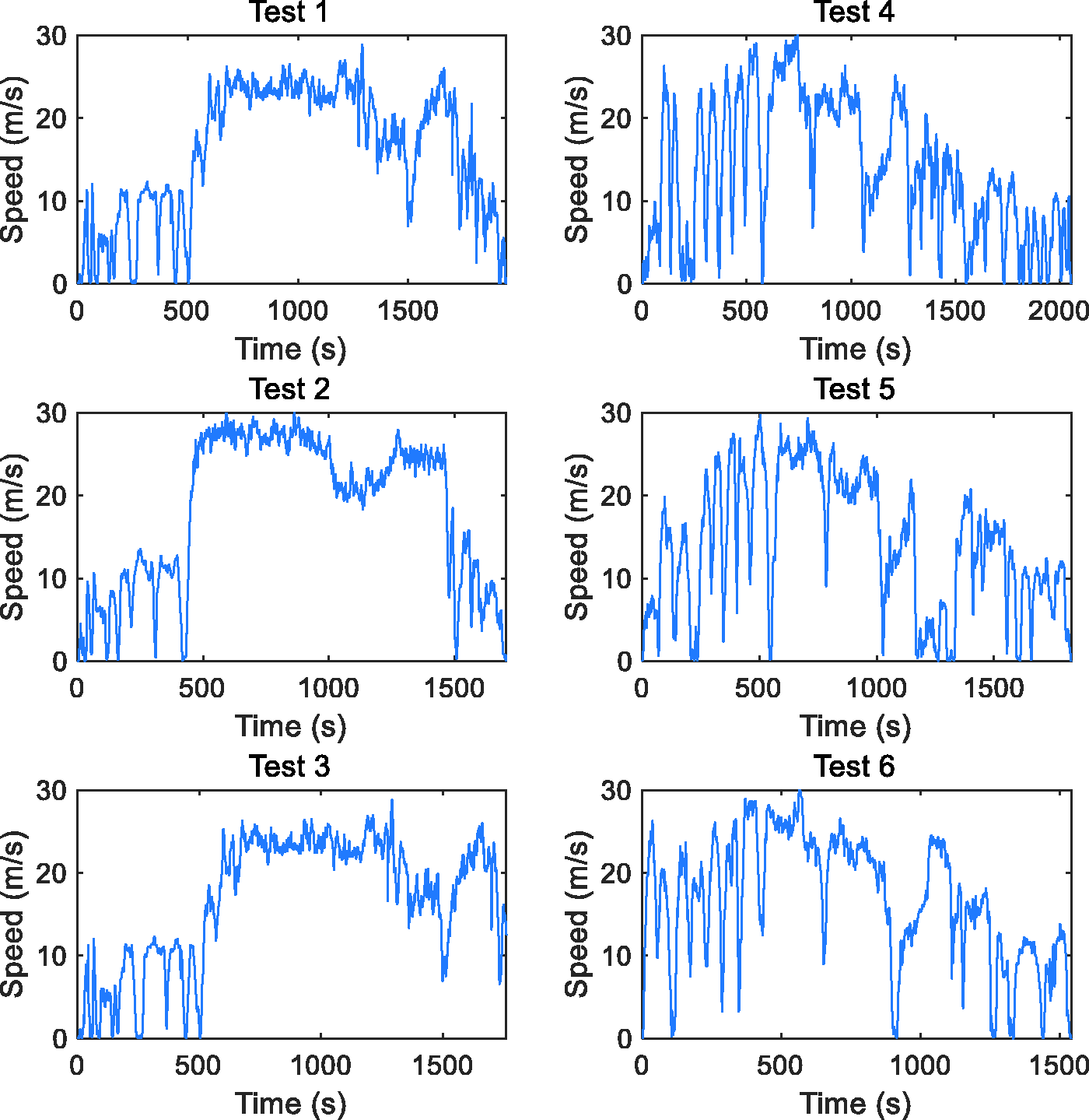
Speed profiles of the six tests: tests 1, 2 and 3 are performed on route A whereas tests 4, 5 and 6 are collected on route B.

Driving pattern clustering based on average speed

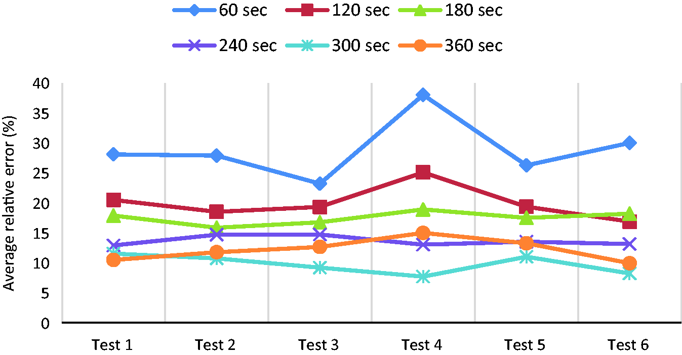
This section presents the results of the clustering method using ‘average speed’ as the only driving feature. The results of ‘average power’ and combination of both of them are also discussed in ‘Driving pattern clustering based on average power’ section and ‘Driving pattern clustering based on both average speed and average power’ section. Figure 11 shows the average relative error of each test using average speed by considering three clusters for different segment lengths. The results demonstrate that the average relative errors of the 60-sec segment length are the highest, ranging from 25% to 40% for different tests, whereas the 300-sec segment length has the smallest errors, ranging from 5% to 15%. Since the 360-sec segment length does not improve the results in comparison to 300-sec, longer segment lengths are not investigated here. To conclude this outcome, when the segment length increases, the energy consumption values in the same cluster become at a similar level. In other words, the variance of energy consumption values in each cluster is smaller, resulting in smaller errors. However, if the segment length is too long, the energy consumption might be less sensitive to a change in the driving pattern.

Figure 11.

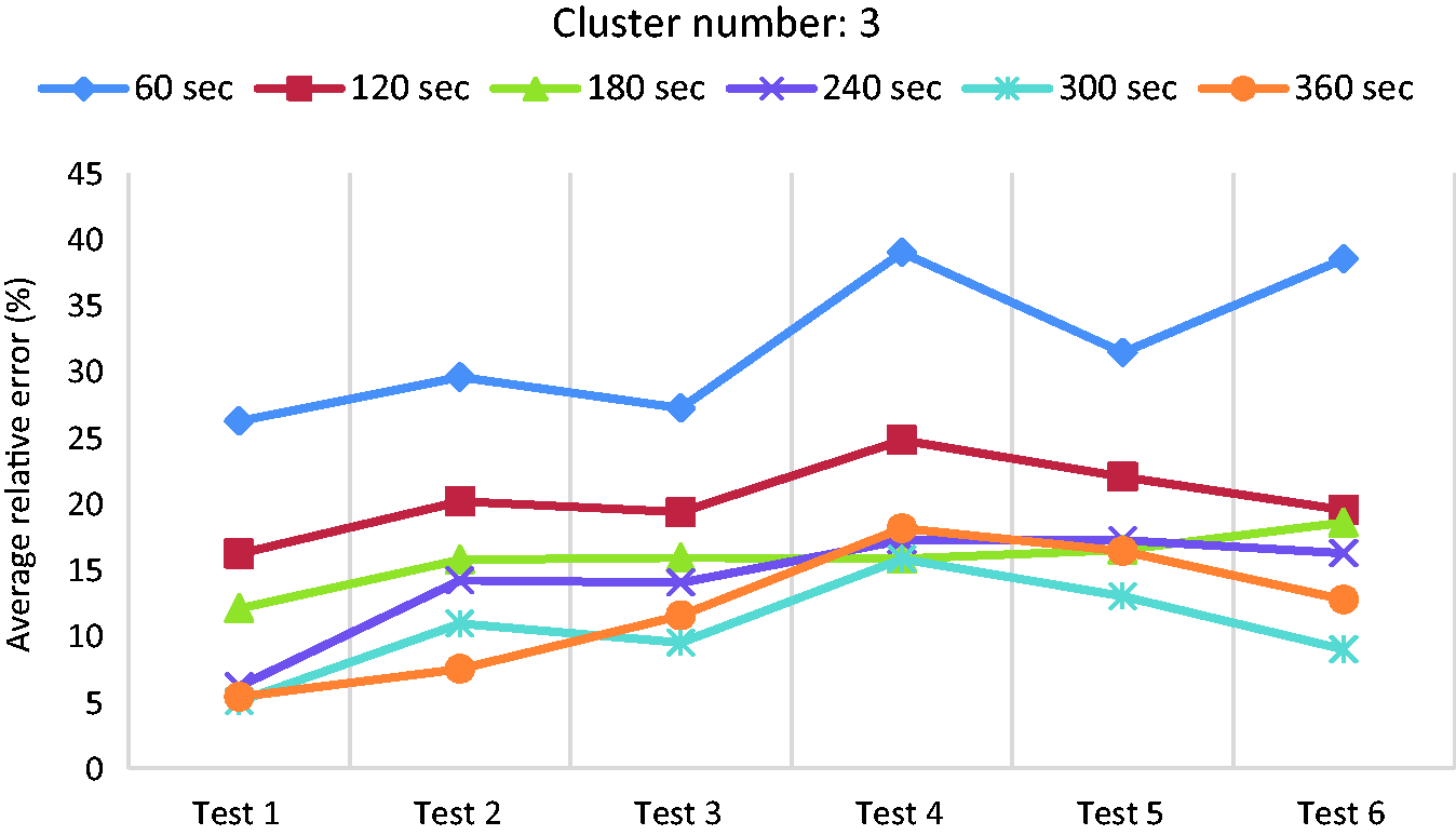
Average error of each test using three clusters based on average speed.

Figures 12 and 13 show the error values in the 4-cluster and 5-cluster cases respectively. As shown in the figures, the two cases have similar trends as that of 3-cluster case. Among all these cases, the 300-sec segment has the lowest errors; therefore, 300-sec (i.e. five minutes history) is chosen as the most suitable length for segmentation with respect to the average relative error. As a summary, the average relative error of different tests in case of 300-sec segment length is shown in Figure 14. The results demonstrate that for most of the tests, the case of 5-cluster has the lowest errors in comparison to the 3-cluster and 4-cluster cases. More than five clusters is not further investigated because the higher the cluster number is, the more transitions between the clusters happen, which can potentially result in more fluctuation in the estimated RDR or in other words, causing confusion for the EV user.

Figure 12.

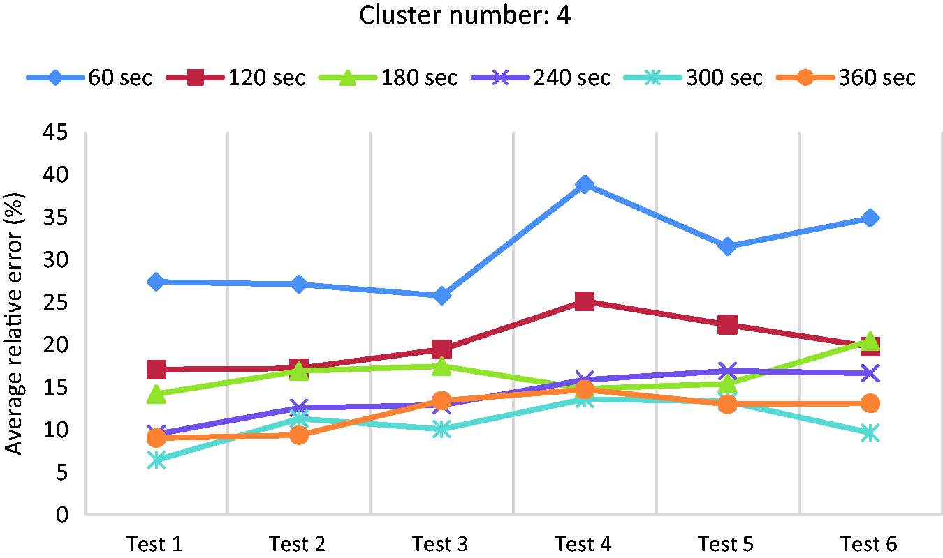
Average relative error for different tests in case of using four clusters and average speed.

Figure 13.

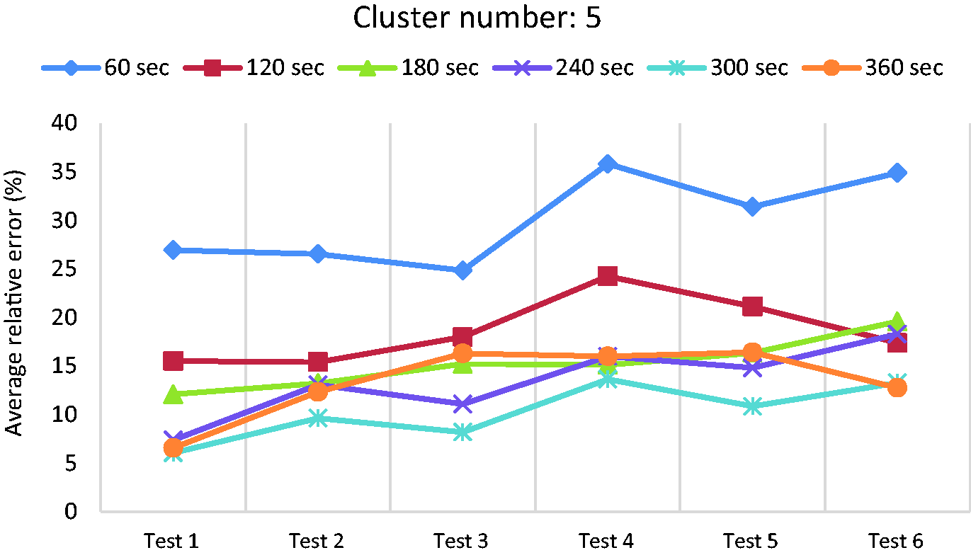
Average relative error for different tests in case of using five clusters and average speed.

Figure 14.

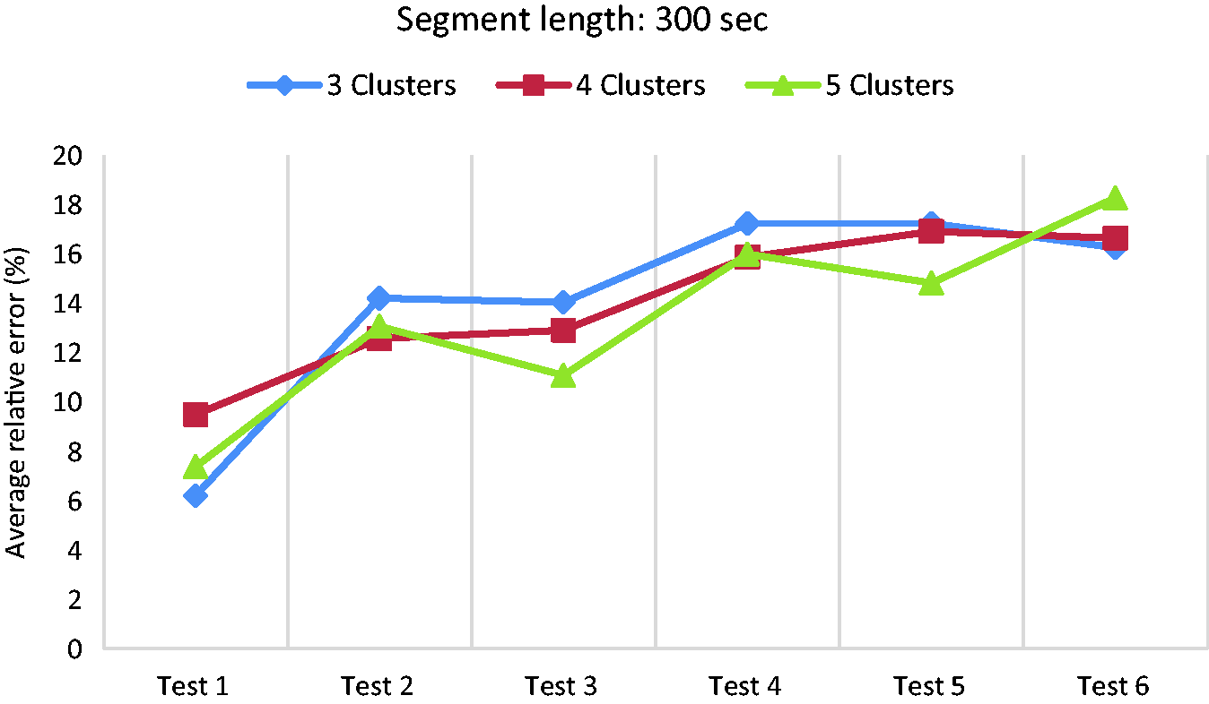
Average relative error for different tests in case of 300-sec segment length using average speed.

From the above analyses, it is concluded that the proposed clustering method works best when considering 300-sec segment length and five clusters using average speed as the only feature. Table 3 contains the error values for the six experimental tests using the proposed method. According to the results, Test 1 has the lowest error of 6.06%, test 4 has the highest error of 13.63% and the average error of all the tests is around 10%.

Table 3.

Average relative error of different tests using average speed as the only feature.

	Test 1	Test 2	Test 3	Test 4	Test 5	Test 6	Average
Average relative error	6.06%	9.64%	8.19%	13.63%	10.86%	13.28%	10.28%

Driving pattern clustering based on average power

In this section, ‘average power’ is used instead of ‘average speed’ as the only feature for driving segment clustering and RDR estimation. Figure 15 shows the errors in the 3-cluster case, where 120-sec segment length causes the highest errors around 20%. A similar trend that was observed and discussed in ‘Driving pattern clustering based on average speed’ section for the average speed, can be found here too. According to the results, the error decreases when the segment length increases. When the cluster number increases to four and five, as shown in Figures 16 and 17, the 300-sec segment length has the lowest error for some tests while for the others, the 360-sec is the best. Since 300-sec and 360-sec have error values in a same range, 300-sec is preferred as it is shorter and thus more sensitive to any quick change in driving pattern. Therefore, 300-sec segment length is chosen as the best choice here too.

Figure 15.

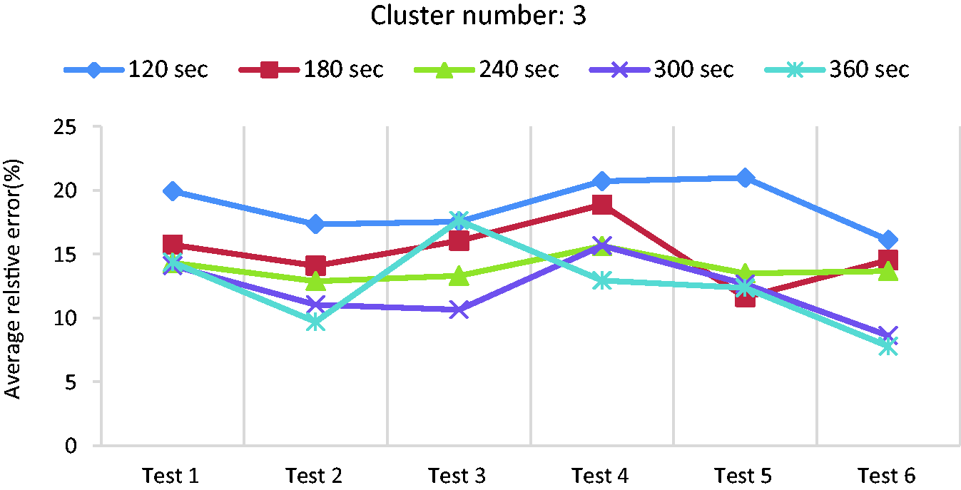
Average relative error for different tests in case of using three clusters and average power.

Figure 16.

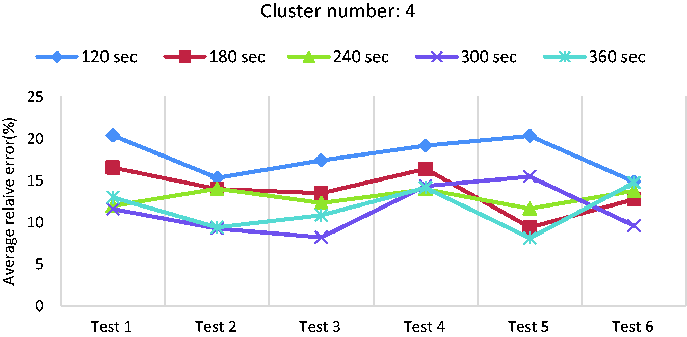
Average relative error for different tests in case of using four clusters and average power.

Figure 17.

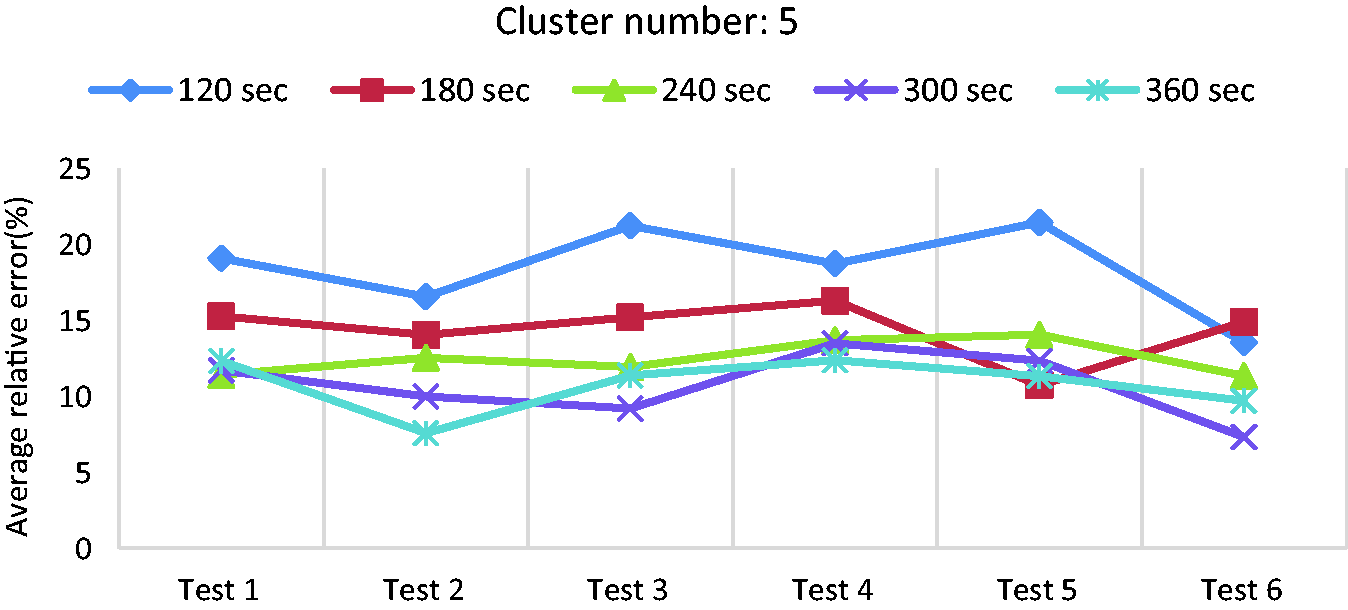
Average relative error for different tests in case of using five clusters and average power.

Figure 18 compares error values using different cluster numbers and average power as the only feature. According to the results, 300-sec segment length and five clusters are selected as the best choices. The error values for different tests using 300-sec segment length and five clusters are presented in Table 4, where the lowest error is 7.32% (i.e. for test-6), the highest error is 11.71% and the average error is around 10%. Compared with that from the average speed, the error is at a similar level.

Figure 18.

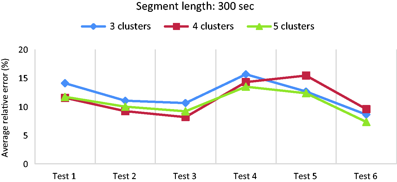
Average relative error for different tests in case of 300-sec segment length using average power.

Table 4.

Average relative error of different tests in case of 300-sec segment length using average power as the only feature.

	Test 1	Test 2	Test 3	Test 4	Test 5	Test 6	Average
Average relative error	11.71%	9.99%	9.19%	13.49%	12.35%	7.32%	10.68%

Driving pattern clustering based on both average speed and average power

In this section, same analysis is performed as explained in ‘Driving pattern clustering based on average speed’ section and ‘Driving pattern clustering based on average power’ section however, by using both features of ‘average speed’ and ‘average power’. The clusters boundaries are defined as explained in ‘Driving pattern clustering based on average speed and average power’ section. Figure 19 shows the average relative error of energy consumption estimation for different tests using both the ‘average speed’ and ‘average power’ features. The results demonstrate that the higher the segment length is, the lower the average errors are; except for the 360-sec segment length that has higher errors than the 300-sec case. Therefore, among all the segment lengths, the best choice seems to be the 300-sec length (i.e. same outcome obtained in previous sections too). Table 5 contains the average relative error values of different tests in case of 300-sec segment length. According to the results, the minimum error is 7.73%, the maximum error is 11.56%, and the average error of all six tests is 9.76%. In comparison to the previous error values presented in Tables 3 and 4, it can be concluded that the use of both ‘average speed’ and ‘average power’ performs slightly better than each individual feature. Although this improvement has been obtained with the cost of double computational effort and memory in real-time. Of course, the use of more features is also possible however, a good design is the one which is based on a proper trade-off between accuracy and simplicity in real-time.

Figure 19.

Average relative error of energy consumption estimation using two features for different segment lengths.

Table 5.

Average relative error of different tests in case of 300-sec segment length and using both average speed and average power.

	Test 1	Test 2	Test 3	Test 4	Test 5	Test 6	Average
Average relative error	11.56%	10.77%	9.23%	7.73%	11.03%	8.25%	9.76%

Figure 20 demonstrates 300-sec segments in a two-dimensional feature space, which includes average speed and average power. All the drive cycles and the real test data (6 tests) are divided into 300-sec segments where each point represents one segment in that figure. Figure 20(a) shows the clusters which are used in this study, as introduced in ‘Driving pattern clustering based on average speed and average power’ section. Since no segment belongs to Cluster 3 according to the definition presented in ‘Driving pattern clustering based on average speed and average power’ section, that useless cluster was eliminated and instead, Cluster 4 is named as Cluster 3 in Figure 20(a). To evaluate the clustering outcomes, a second technique called k-means clustering⁵² is used as a benchmark too. K-means clustering technique has been used before for driving segment clustering in the literature.³⁹ Figure 20(b) shows the clustering results of the same data using the k-means method. As shown in the figure, there is not much difference between the clustering outcomes using the two techniques, which validates the proposed technique of this study. Although both techniques generate same results, we preferred to use the first method, which was presented in ‘Driving pattern clustering based on average speed and average power’ section, because of its simplicity for real-time applications.

Figure 20.

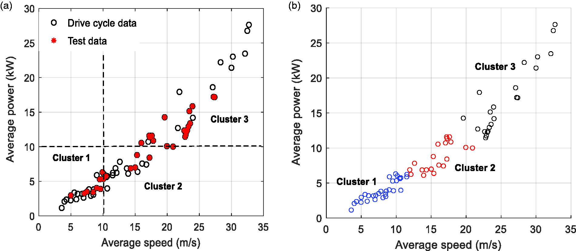
Driving segments clustering: (a) clustering based on speed/power thresholds, (b) clustering using k-means method.

Results summary and comparison

Clustering results

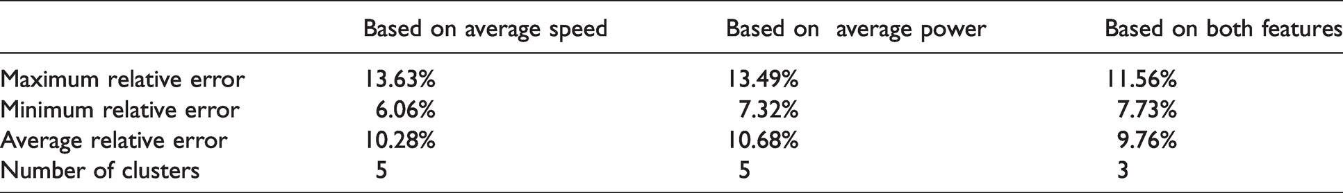
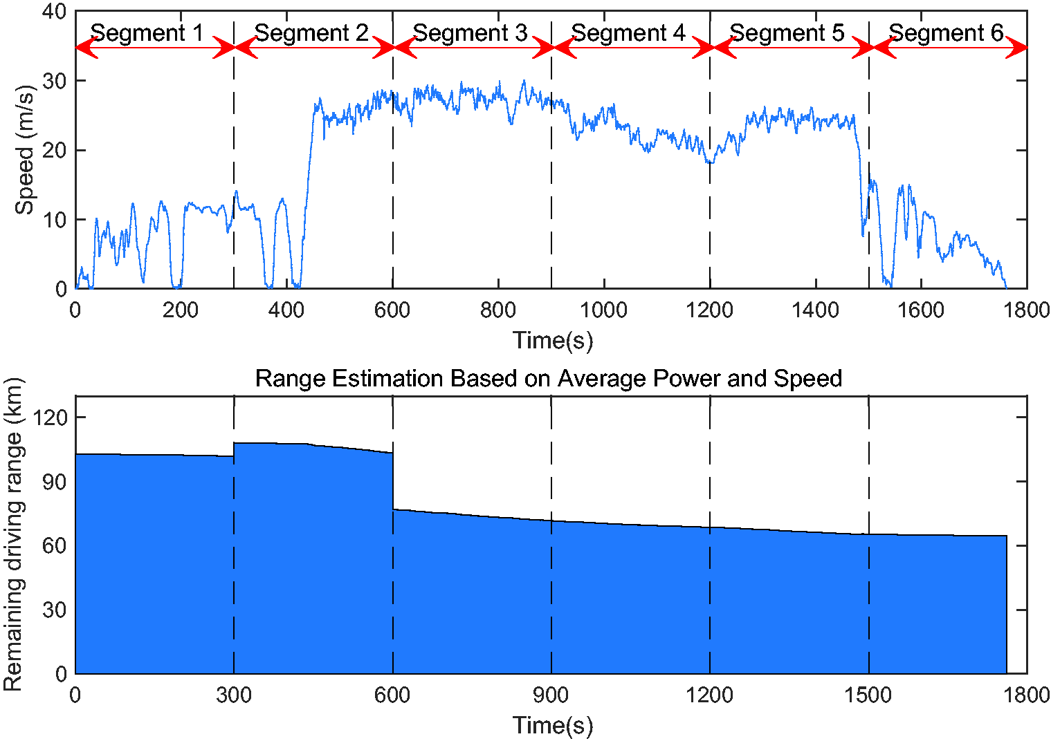
The average relative error values, which are obtained from different clustering solutions, are summarised in Table 6. The results demonstrate that the clustering solution based on both ‘average speed’ and ‘average power’ has the lowest values of maximum and average error. The proposed clustering solution based on the two features uses only three clusters, while the other two solutions use five clusters. Those selections are made based on the results of different cluster numbers, which were presented earlier in Figures 14 and 18. The use of less clusters has the advantages of simplicity and less RDR estimation fluctuations (i.e. due to less cluster change) in real-time too. Considering Test 3 as an example shown in Figure 21; during that test, the vehicle has travelled on an urban road at the first 400 sec and then it has moved to a highway. Using the clustering method based on both features, there is only one cluster change during that test, which is detected by the algorithm and the RDR estimation is adjusted accordingly.

Table 6.

Average relative error of energy consumption estimation using different clusters and features.

	Based on average speed	Based on average power	Based on both features
Maximum relative error	13.63%	13.49%	11.56%
Minimum relative error	6.06%	7.32%	7.73%
Average relative error	10.28%	10.68%	9.76%
Number of clusters	5	5	3

Figure 21.

RDR estimation during Test 3 based on average power and average speed.

It should be noted that the driving condition can be recognised only after 300th sec of the journey. The initial driving condition cluster is assumed to be cluster number 1 at the first 300 sec of each journey (the first segment), which means the RDR estimation is performed based on energy consumption of cluster number 1 at the beginning. The reason of choosing the first cluster is that usually the driving pattern has low speed and power demand just after starting an EV. After the first segment, the driving condition is updated based on the extracted features.

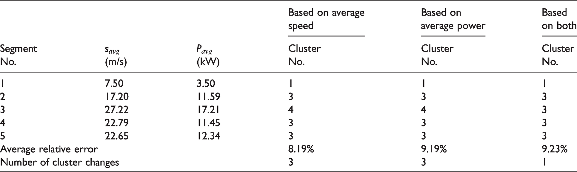
Figures 21 and 22 show the estimated RDR using the proposed clustering method based on: (i) two features, (ii) average power, and (iii) average speed respectively. According to Figure 21, the estimated RDR drops from 110 km to around 75 km when the estimator recognises the change in driving pattern from urban driving to highway driving. After that, the estimated range drops steadily as the recognised driving pattern keeps unchanged and the battery state-of-charge decreases gradually. However, by using only one of the ‘average power’ or ‘average speed’, the estimated range has more fluctuation as shown in Figure 22(a) and (b). Table 7 summarises the results in form of the number of cluster changes and average relative error using three different clustering approaches. Since the relative error of energy consumption estimation using all the three clustering approaches is at a similar level (i.e. around 9%), therefore, we can conclude that the clustering method using both features is preferred because of fewer cluster changes. Again it should be highlighted here that a proper trade-off is necessary between EV user’s comfort (by providing a more consistent estimation) and sensitivity to a quick change in driving pattern (i.e. higher RDR accuracy). As discussed earlier, one clustering solution can bring a higher accuracy in RDR but with the cost of more fluctuations on the dashboard. The extreme example of this case is a pure RDR estimator that works based on instantaneous energy consumption, which is ‘too accurate’ to be useable in practice. On the other hand, another clustering solution can bring a higher robustness in RDR but with the cost of less sensitivity to a quick change in driving pattern (i.e. less accuracy). The extreme example of this case is a RDR estimator that uses only one cluster (i.e. constant Wh/km) and a long time window of the motion history. This study was aimed at exploring other alternative solutions between those extremes by proposing the idea of driving pattern recognition in real-time.

Figure 22.

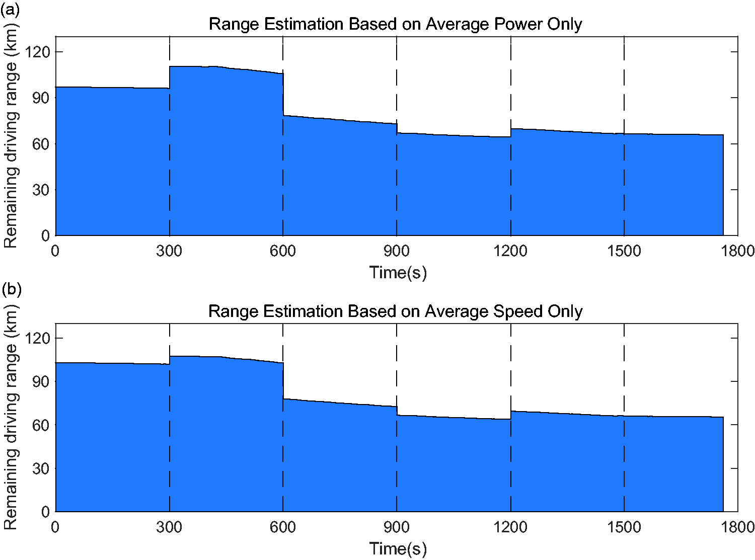
RDR estimation during Test 3: (a) based on average power, and (b) based on average speed.

Table 7.

Number of cluster changes and average relative error during Test 3 using three different clustering approaches.

			Based on averagespeed	Based on average power	Based on both
SegmentNo.	$s_{avg}$ (m/s)	$P_{avg}$ (kW)	Cluster No.	ClusterNo.	ClusterNo.
1	7.50	3.50	1	1	1
2	17.20	11.59	3	3	3
3	27.22	17.21	4	4	3
4	22.79	11.45	3	3	3
5	22.65	12.34	3	3	3
Average relative error			8.19%	9.19%	9.23%
Number of cluster changes			3	3	1

Energy consumption prediction results evaluation against a benchmark method

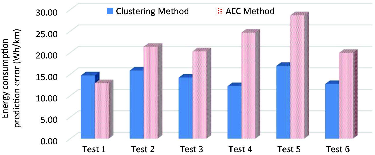
As a complementary analysis, performance of the proposed method is compared with a standard benchmark RDR estimation technique. Average Energy Consumption (AEC) method is used as the benchmark in which the EV energy consumption per km is estimated according to the vehicle specifications published by the manufacturer. Particularly for BMW i3, a new reference is added which includes the average energy consumption of that car, which is around 169 Wh/km.⁴⁶ That reference number is then used in the benchmark method (i.e. AEC) for energy consumption prediction. The results are calculated for all six test profiles using both clustering and AEC methods. Comparison between the outcomes is presented in Figure 23, which demonstrates the proposed driving pattern clustering technique outperforms the standard benchmark technique. Except for Test 1 where the AEC method works well, in all other cases, driving pattern clustering improves the results. The reason that AEC works well for Test 1, is that the energy consumption of that particular test is accidentally very close to the nominal value of 169 Wh/km. Indeed, the driving pattern clustering technique is able to distinguish between different driving segments however, the AEC is handling them in a same way. That means the AEC method generates higher errors when the real energy consumption is more far from the nominal value.

Figure 23.

Energy consumption prediction error using AEC and driving pattern clustering methods.

By considering the average of all six tests, the proposed technique improves the energy consumption prediction results around 7 Wh/km in comparison to the AEC method. This improvement can be even more if we could consider the effects of variations in passenger weight, road gradient, tyre pressure, and the air conditioning system. All of these factors directly affect the average power, which is used as a feature in our driving pattern recognition system. So, the proposed technique will be able to react to them however, the AEC method cannot.

Conclusions

This study was aimed at creating a multi-mode EV range estimator based on driving pattern recognition. By assuming that the battery capacity is known, range estimation was presented in form of energy consumption prediction (Wh/km). The proposed technique is expected to fill the gap between the model-based range estimation methods, which are more accurate but need more data and computational effort, and the history-based range estimators, which are easier to be implemented in real-time but less accurate. The history-based methods have been preferred in this study because of their less complexity (i.e. model-free) and being easy for implementation in real-time. Subsequently, an EV range estimation strategy was proposed that firstly recognise the driving pattern over the last few minutes of vehicle motion, and then classifies the driving pattern into one of the predefined clusters (driving modes). The energy consumption predictor uses that information until it recognises a change in the driving pattern, which is the time to switch to another mode. Different number of clusters and segment lengths (ranging from 60 to 360 seconds) were studies to find the optimum segment length and the number of driving modes. Average speed and average power were chosen to be used as driving features. According to the results, by considering segment length of 300 seconds and three clusters, an average relative error of around 9% was obtained for EV energy consumption prediction when compared with experimental data. Considering the fact that an EV range can be affected by a number of factors, the proposed range estimator demonstrated a promising level of accuracy. One important feature of the proposed technique was the ability to be implementable in real-time. That is against many other high accuracy model-based estimators in the literature, which are more accurate but not practical.

In addition to driving conditions, other factors could also introduce uncertainties, which make the EV energy consumption prediction even more challenging. For example, the range of EV drops under cold or hot climates. The primary contributor to range decrease is the cabin climate control system. To maintain the occupant's comfort within a thermal comfort zone, heating, ventilation, and air conditioning (HVAC) system is utilised, which is the second most energy-consuming system after the electric motor. Therefore, it should be considered as an additional element when developing EV RDR estimation algorithms. Moreover, the effect of battery thermal behaviour should be investigated as well to improve the RDR estimation results.

Footnotes

Declaration of Conflicting Interests

The author(s) declared no potential conflicts of interest with respect to the research, authorship, and/or publication of this article.

Funding

The author(s) received no financial support for the research, authorship, and/or publication of this article.

ORCID iD

Abbas Fotouhi

References

Hong

Wang

Zhang

, et al. Research on integration simulation and balance control of a novel load isolated pure electric driving system. Energy 2019; 189: 116220.

Shi

Pan

Wang

, et al. Battery electric vehicles: what is the minimum range required? Energy 2019; 166: 352–358.

Sehar

Pipattanasomporn

Rahman

, et al. Demand management to mitigate impacts of plug-in electric vehicle fast charge in buildings with renewables. Energy 2019; 120: 642–651.

Pevec

Babic

Carvalho

, et al. Electric vehicle range anxiety: an obstacle for the personal transportation (r)evolution? In: 2019 4th International Conference on Smart and Sustainable Technologies, SpliTech 2019, Split, Croatia, 18–21 June 2019.

Heath

Sant

Allen

Do you feel lucky? Why current range estimation methods are holding back EV adoption. Thiruvananthapuram: IET Conference Publications, 2013.

Smuts

Scholtz

Wesson

A critical review of factors influencing the remaining driving range of electric vehicles. In: 2017 1st international conference on next generation computing applications NextComp 2017. 2017, Mauritius: IEEE. pp.196–201.

Franke

Neumann

Bühler

, et al. Experiencing range in an electric vehicle: understanding psychological barriers. Appl Psychol 2012; 61: 368–391.

Zhang

Wang

Kobayashi

, et al. Remaining driving range estimation of electric vehicle. In: 2012 IEEE International Electric Vehicle Conference, IEVC 2012, Greenville, SC, 4–8 March 2012.

Ferreira

Monteiro

Afonso

JL.

Dynamic range prediction for an electric vehicle. In: 2013 world electric vehicle symposium and exhibition, Barcelona, Spain, 17–20 November 2013.

10.

Varga

Sagoian

Mariasiu

Prediction of electric vehicle range: a comprehensive review of current issues and challenges. Energies 2019; 12: 946.

11.

Moure

Roche

Mammetti

Range estimator for electric vehicles. In: 2013 world electric vehicle symposium and exhibition, Barcelona, Spain, 17–20 November 2013.

12.

Wai

Rong

Morris

Simulation of a distance estimator for battery electric vehicle. Alexandria Eng J 2015; 54: 359–371.

13.

Çeven

Albayrak

Bayır

Real-time range estimation in electric vehicles using fuzzy logic classifier. In: Dr. N. Velmurugan (Ed) Computers and electrical engineering, May, 2020. Vol.83. Amesterdam: Elsevier. p.106577.

14.

Hong

Park

Chang

Accurate remaining range estimation for electric vehicles. In: Proceedings of the Asia and South Pacific design automation conference, ASP-DAC, Macao, 25–28 January 2016, pp.781–786. Piscataway, NJ: IEEE.

15.

Grewal

Darnell

PM.

Model-based EV range prediction for electric hybrid vehicles. Thiruvananthapuram: IET Conference Publications, 2013.

16.

Bolovinou

Bakas

Amditis

, et al. Online prediction of an electric vehicle remaining range based on regression analysis. In: 2014 IEEE international electric vehicle conference, IEVC, Florence, Italy, 17–19 December 2014.

17.

Vaz

Nandi

AKR

Landers

, et al. Electric vehicle range prediction for constant speed trip using multi-objective optimization. J Power Sources 2015; 275: 435–446.

18.

Sun

Zhang

, et al. A machine learning method for predicting driving range of battery electric vehicles. J Adv Transport 2019; 2019: 1–14.

19.

Rahimi-Eilchi

Chow

MY.

Big-data framework for electric vehicle range estimation. In: IECON proceedings (Industrial Electronics Conference), Dallas, TX, 29 October–1 November 2014.

20.

Aktekin

Gumus

Haspolat

, et al. Average consumption-based range estimator design for a human-electric hybrid vehicle. In: ELECO 2019 11th international conference on electrical and electronics engineering. 2019, Bursa: IEEE. pp.840–844.

21.

Vatanparvar

Faezi

Burago

, et al. Extended range electric vehicle with driving behavior estimation in energy management. IEEE Trans Smart Grid 2019 10(3), 2959–2968.

22.

Wang

Besselink

Nijmeijer

Electric vehicle energy consumption modelling and prediction based on road information. Wevj 2015; 7: 447–458.

23.

Sarrafan

Sutanto

Muttaqi

, et al. Accurate range estimation for an electric vehicle including changing environmental conditions and traction system efficiency. IET Electr Syst Transport 2017; 7: 117–124.

24.

Tesla Company. Model S owner’s manual. California: Tesla Company, 2019, p.208.

25.

Lemon

Booklet

, SU Nissan leaf owner’s manual. 2010, US: Nissan.

26.

Ideal

RZ.

Renault Zoe. Ideal.Es/Granada. 2017. (April): 5–7.

27.

Barcellona

Grillo

Piegari

A simple battery model for EV range prediction: theory and experimental validation. In: 2016 international conference on electrical systems for aircraft, railway, ship propulsion and road vehicles and international transportation electrification conference, ESARS-ITEC 2016, Toulouse, France, 2-4 Nov. 2016. IEEE.

28.

German

Shili

Desreveaux

, et al. Dynamical coupling of a battery electro-thermal model and the traction model of an EV for driving range simulation. IEEE Trans Veh Technol 2020; 69: 328–337.

29.

Oliva

Weihrauch

Bertram

Model-based remaining driving range prediction in electric vehicles by using particle filtering and Markov chains. In: 2013 world electric vehicle symposium and exhibition, EVS 2014. Piscataway, NJ: IEEE, 2014, pp.1–10.

30.

Oliva

Weihrauch

Bertram

A model-based approach for predicting the remaining driving range in electric vehicles. In: PHM 2013 proceedings of the annual conference of the prognostics and health management society, 2013, Barcelona: PHM Society. pp.438–448.

31.

Pan

Dai

Chen

, et al. Driving range estimation for electric vehicles based on driving condition identification and forecast. AIP Adv 2017; 7: 105206.

32.

Liu

, et al. Remaining driving range estimation for electric vehicles through information fusion method. Amm 2014; 668–669: 641–646.

33.

Adnane

Nguyen

B-H

Khoumsi

, et al. Driving mode predictor-based real-time energy management for dual-source electric vehicle. IEEE Trans Transport Electrification 2021; In Press. DOI:10.1109/TTE.2021.3059545.

34.

Sonalikar

Shelke

SD.

Estimation of remaining range of electric vehicle using Kalman filter. In: Proceedings of the international conference on inventive research in computing applications, ICIRCA 2018. Piscataway, NJ: IEEE, 2018, pp.632–636.

35.

Grubwinkler

Hirschvogel

Lienkamp

Driver- and situation-specific impact factors for the energy prediction of EVs based on crowd-sourced speed profiles. In: IEEE intelligent vehicles symposium, proceedings. Piscataway, NJ: IEEE, 2014. 1069–1076.

36.

Ericsson

Independent driving pattern factors and their influence on fuel-use and exhaust emission factors. Transport Res Part D: Transport Environ 2001; 6: 325–345.

37.

Xie

Tian

, et al. A hybrid method combining Markov prediction and fuzzy classification for driving condition recognition. IEEE Trans Veh Technol 2018; 67: 10411–10424.

38.

Fotouhi

Montazeri

Jannatipour

Vehicle’s velocity time series prediction using neural network. Int J Autom Eng 1: 21–28.

39.

Montazeri-Gh

Fotouhi

Naderpour

Driving patterns clustering based on driving feature analysis. Proc IMechE, Part C: J Mechanical Engineering Science 2011; 225: 1301–1317.

40.

Feng

Liu

Chen

Driving pattern recognition for adaptive hybrid vehicle control. SAE Int J Alt Power 2012; 1: 169–179.

41.

Zhang

Xiong

Adaptive energy management of a plug-in hybrid electric vehicle based on driving pattern recognition and dynamic programming. Appl Energy 2015; 155: 68–78.

42.

Jeon

Park

, et al. Multi-mode driving control of a parallel hybrid electric vehicle using driving pattern recognition. J Dyn Syst Measure Control, Trans ASME 2002; 124: 141–149.

43.

Langari

Won

JS.

Intelligent energy management agent for a parallel hybrid vehicle – part I: system architecture and design of the driving situation identification process. IEEE Trans Veh Technol 2005; 54: 925–934.

44.

Neubauer

Brooker

Wood

Sensitivity of plug-in hybrid electric vehicle economics to drive patterns, electric range, energy management, and charge strategies. J Power Sources 2013; 236: 357–364.

45.

BMW Group. BMW U.S media information technical data 2014 BMW i3, 2014.

46.

BMW-i3, https://ev-database.uk/car/1104/BMW-i3 (accessed 5 July 2021).

47.

Miri

Fotouhi

Ewin

Electric vehicle energy consumption modelling and estimation – a case study. Int J Energy Res 2021; 45: 501–520.

48.

Fotouhi

Montazeri-Gh

Tehran driving cycle development using the k-means clustering method. Sc Iran 2013; 20: 286–293.

49.

Montazeri-Gh

Fotouhi

Traffic condition recognition using the k-means clustering method. Sci Iran 2011; 18: 930–937.

50.

Montazeri

Fotouhi

Naderpour

Driving segment simulation for determination of the most effective driving features for HEV intelligent control. Veh Syst Dyn 2012; 50: 229–246.

51.

Fotouhi

Shateri

Shona Laila

, et al. Electric vehicle energy consumption estimation for a fleet management system. Int J Sustain Transport 2020; 15: 40–54.

52.

Lloyd

SP.

Least squares quantization in PCM. IEEE Trans Inform Theory 1982; 28: 129–137.

A multi-mode electric vehicle range estimator based on driving pattern recognition

Abstract

Keywords

Introduction

Range estimation strategy

Driving data segmentation and energy consumption calculation

EV energy consumption model

Sample data for offline energy consumption calculation

Energy consumption calculation

Driving pattern clustering

Driving pattern clustering using average speed

Driving pattern clustering based on average power

Driving pattern clustering based on average speed and average power

RDR estimation and validation

Validation approach

Average relative error

Real driving speed profiles

Driving pattern clustering based on average speed

Driving pattern clustering based on average power

Driving pattern clustering based on both average speed and average power

Results summary and comparison

Clustering results

Energy consumption prediction results evaluation against a benchmark method

Conclusions

Footnotes

Declaration of Conflicting Interests

Funding

ORCID iD

References