Sage Journals: Discover world-class research

Abstract

Helical springs have been widely used in various engineering applications for centuries. For many years, there is no significant development in the design methods of helical springs. Recently, a renewed interest is raised from the industry in exploring new designs for the helical springs with novel configurations due to the requirements of customised properties, such as specific spring stiffness and natural frequency for better performance of valve train systems. In this paper, an innovative method which combines the techniques of Finite Element Analysis (FEA), constrained Latin Hypercube sampling (cLHS) and Genetic Programming (GP) is developed to design and analyse helical springs with arbitrary shapes. cLHS method is applied to generate 300 sets of spring samples within a constrained design domain, and FE analysis is conducted on these spring samples. Two meta-models are developed from the 300 sets of FE results by using GP. They successfully describe the relationships between the design parameters and the overall mechanical performances including compression force and fundamental natural frequency of helical springs. The results show that the developed models have robust abilities on designing helical springs with arbitrary shapes, which significantly expands the design domain of the engineering design methods and potential for precise optimization of helical springs.

Keywords

Spring design machine learning computer-aided design data-driven design design of experiments

Introduction

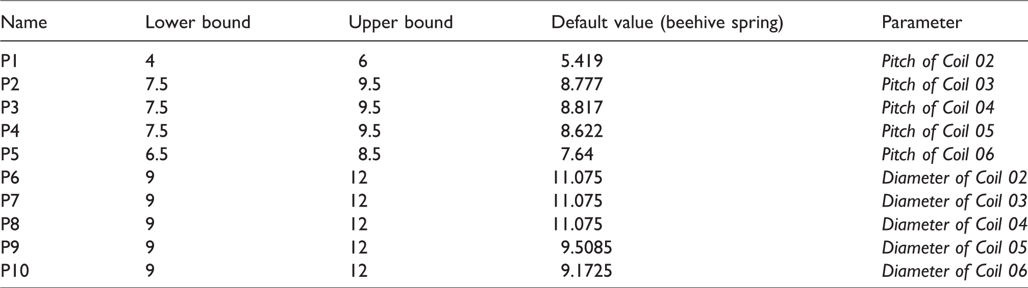
Engineering design of machine elements is one of the most important tasks in engineering sectors. However, many of the existing design methods are still experience-based or on the basis of classic theories of machines and mechanisms, which are not very suitable to design machine elements with specified properties. Helical spring is a typical example. Helical spring, which is a common form of mechanical springs, is an essential component in many mechanical systems, for instance, valve train system. In an internal combustion (IC) engine, valve springs are the most flexible components, which must guarantee the precise and high-efficient return motions of valves. Good designs can bring many benefits, such as high spring strength, low fuel consumption and enhanced high speed performances, etc.,^1–4 while poor designs of valve springs may lead to severe spring damage and malfunction of engine. Currently, the designs and optimizations of helical springs are usually based on empirical equations that have been proposed for around a decade. 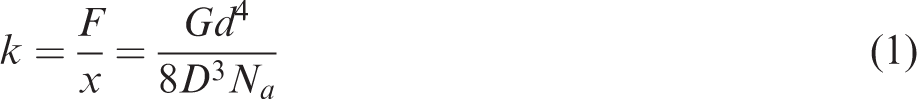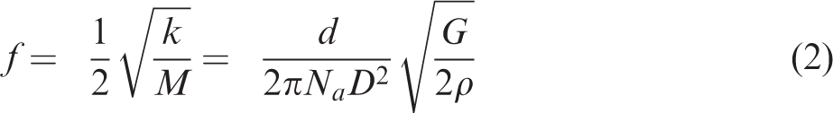The most commonly employed equations are the ones developed by Wahl⁵ for calculating the spring stiffness by equation (1), the first order natural frequency by equation (2) and the maximum shear stress by equation (3).

k = \frac{F}{x} = \frac{G d^{4}}{8 D^{3} N_{a}}

(1)

f = \frac{1}{2} \sqrt{\frac{k}{M}} = \frac{d}{{2 π N}_{a} D^{2}} \sqrt{\frac{G}{2 ρ}}

(2)

τ_{m} = \frac{8 F D}{π d^{3}} K_{c}

(3)

where k is spring stiffness, F is external loading, x is compression, G is shear modulus, d is wire diameter, D is spring diameter, M is active mass, Na is number of active coils, τ_m is maximum shear stress and Kc is Wahl correction factor. These equations are widely used in design and optimization of the helical springs in most of existing studies. Mancini and Piziali⁶ developed a straightforward method to optimize the life and strength of compression helical springs. equation (3) was used to express the essential relationships between the maximum shear stress and the geometrical properties of springs, when equation (2) was used as one of the physical constraints. Another paper published by Muhr⁷ was to develop a new technology for designing engine valve springs. A 13% reduction of the maximum shear stress was achieved by applying equation (3), and a 35% reduction in required installation heights was achieved by applying equation (1). Similarly, Aurel⁸ presented a study of exploring the optimal design of a helical spring with minimum spring mass. In the study, equation (3) was applied as the constraints for meeting the allowable fatigue stress. A 16% reduction of spring mass was attained by the optimised design. A study on optimal design of helical springs was published by Pöllänen and Martikka.⁹ It aimed to minimize the wire volume and spring stiffness, whilst to ensure a low level of spring surging and a reliable long fatigue life. They used equations (1) to (3) to formulate the relationships between physical properties and spring force F, natural frequency f, maximum shear stress τ_m respectively. Eventually, a static finite element simulation was conducted to validate the analytical results. The proposed methods were later employed by Taktak et al.¹⁰ to optimize the spring mass and the natural frequencies of a cylindrical helical spring, by Zheng et al.¹¹ to reduce the oscillation amplitude and the valve impact force and by Qimin¹² to minimize the weight of a helical spring. It can be concluded, therefore, that these theoretical equations are capable of optimizing design of conventional helical springs. However, the equations were proposed on the basis of linear assumptions that assume very small pitch angle and spring index. In addition, the number of active coils Na is assumed to be a constant neglecting the effects of coils clash. In practice, these assumptions restrict the design domain of helical springs significantly. Hence, the current design and optimization methods for helical springs can only involve three simple categories, which are the normal type (Figure 1(a)), the conical type (Figure 1(b)) and the beehive type (Figure 1(c)). These types of helical springs possess linear geometrical properties. For instance, the coil diameter of the normal type is always a constant, and the changing rates of the coil diameters of the conical and the beehive types are always constants. Besides, the spring pitches of these three types are constant as well. However, it has been proved in previous research⁴ that the existing linear theories fail to accurately describe the behaviour of specific high performance helical springs with nonlinear properties. Especially, when coils clash exists, the actual magnitude of spring forces can be 3 times larger than that calculated by the analytical models based on these linear spring theories. Consequently, the conventional linear theory of springs is not suitable to be used to design new high-performance helical springs with specific properties.

Figure 1.

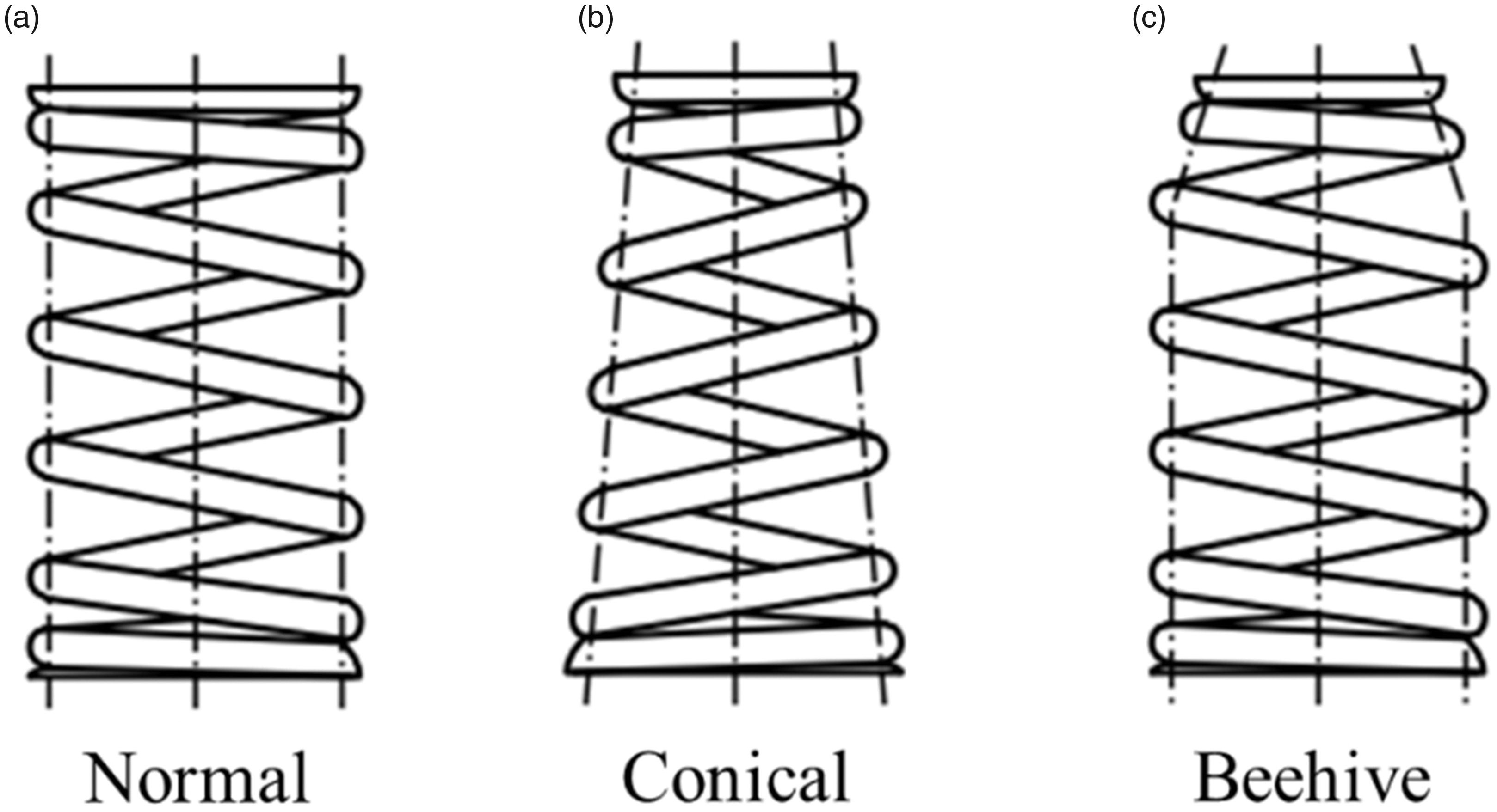
General types of helical springs concerned by existing spring optimization methods. (a) Normal type, (b) Conical type and (c) Beehive type.

In order to describe the nonlinearities of helical springs, the relationships between their physical properties and nonlinear geometries need to be formulated. It is usually extremely difficult to be achieved by using theoretical and empirical equations. On the contrary, the genetic programming (GP) is a specialized technique for formulating nonlinear relationships. The concept of GP was firstly proposed by Cramer¹³ in 1985. It soon attracted considerable attentions due to its robust ability of formulating nonlinear relationships between multiple parameters and ultimate outcomes. Unlike the other black-box machine learning techniques, like artificial neuro network (ANN) which can hardly achieve internal information of a model,¹⁴ GP is a straightforward method to implement symbolic regression to identify possible underlying mathematical expressions. So far, GP has been widely reported to be successfully applied in developing analytical expression for cold-formed steel,¹⁵ deformation modulus of rock,¹⁶ torsional strength of concrete beam¹⁷ and the bond strength of carbon fibre reinforced polymers (CFRPs).¹⁸ In addition, LHS (Latin Hypercube sampling) and GP coupled techniques were used in studies^19,20 to predict the principal stress of a piezoelectric flex transducer, where successful new design was obtained based on the developed method. In these studies, the GP method demonstrated its significant advantage in high prediction accuracy over empirical equations, conventional design codes and traditional multi-regression methods. Similar to the above studies, the design and optimization of helical springs also face the same problem that the conventional empirical and theoretical equations are unable to describe the realistic nonlinear properties. However, according to the author’s best knowledge, there is no existing research has employed GP or similar machine learning techniques in analysis and development of helical springs.

In this study, an innovative design method, which combines finite element analysis (FEA), constrained Latin Hypercube sampling (cLHS) and Genetic Programming (GP) techniques, is developed to improve the accuracy of design and to expend the design domain of helical springs. Firstly, a FE model is developed to simulate the working status of helical springs. In order to satisfy the requirement of sample numbers, a new DoE technique cLHS, which is more flexible than the normal LHS, is implemented to generate design points for FE simulations. Then, the results of FE simulations are used to develop a GP model. To validate both the FE model and the GP models, compression tests are conducted on real manufactured springs. Finally, a sensitive study has been done for analysis the effects of the design parameters. The results show the developed GP models can include essential non-linear effects in analysis and accurately describe the properties of the spring. More importantly, the visible spring formulas generated by GP models could be potentially used as a tool for precise optimization of helical springs in practice.

Methodology

Parametric FE model

The benchmark helical spring used in this study is a beehive valve spring (manufactured by Force Technology Ltd, UK), as shown in Figure 2 left. The valve spring is used in high-speed engines of sports cars. The material for manufacturing the spring is super clean spring steel with the type code of Oteva 90, which has density of 7850 kg/m³, Young’s modulus E of 206 GPa and Shear modulus G of 79.6 GPa. Figure 2 shows the comparisons between the design specifications and the 3D scan data of the beehive spring. It can be seen that the curves of design specifications are linear. However, a nonlinear spring geometry is generated in the process of manufacturing. It means the conventional design theories have ignored the error introduced from the manufacturing process. Consequently, it is impossible to design springs with accurate and specific properties, which are requested by high-end mechanical system. To analyse realistic mechanical performance of the springs, the 3D scanning data is used in all analysis of this paper.

Figure 2.

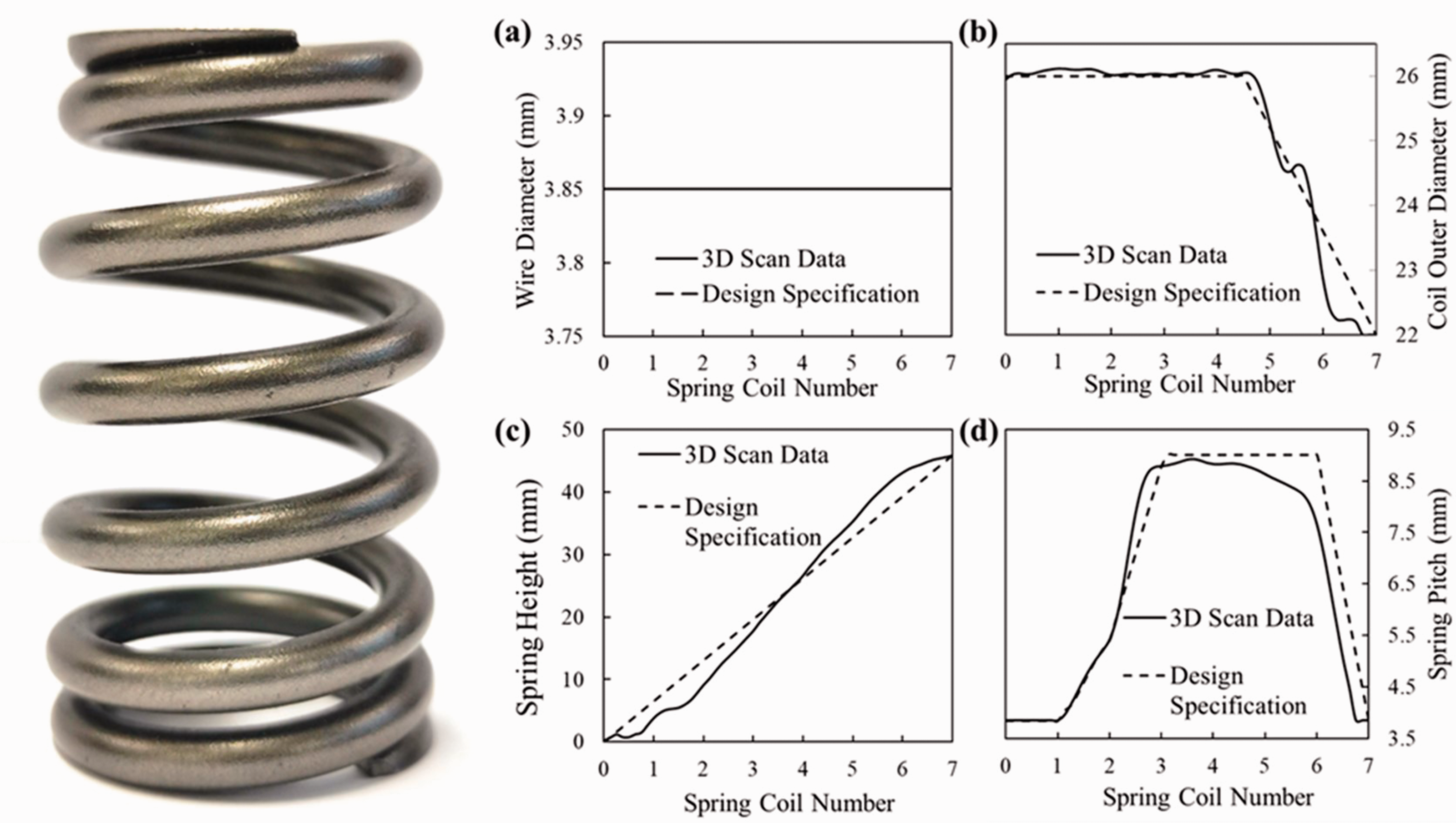
The beehive valve spring manufactured by Force Technology Ltd (Left). Design specification and 3D scan Data of the beehive valve spring (Right).

The numerical spring model in this study is developed using Ansys Workbench based on the 3D scanning data. To describe the geometry model parametrically, 10 geometric parameters (P1 to P10) are defined for the spring model in Figure 3(a) where P1–P5 represent the spring pitches of coil 02–06 and P6–P10 represent the spring diameters of coil 02–06. The geometric model is then used in the FE analysis as shown in Figure 3(b). The meshing strategy and boundary conditions are the same as the ones used in the author’s previous study.⁴ The coils 02 to 06 are meshed by hexahedron elements to reduce the computing time. The end coils 01 and 07 are meshed using tetrahedron elements for their unique shapes. Mesh sensitivity analysis is also conducted on the developed FE model as shown in Table 1. Both the spring force and natural frequency results are converged at 1 mm element size. So, 1 mm element size is defined in the FE spring model and there are in total 70,475 elements and 160500 nodes. In addition, there are two flat surfaces on the end coils (coil 1 and 7) as the manufactured spring is grounded (Figure 3(b)).

Figure 3.

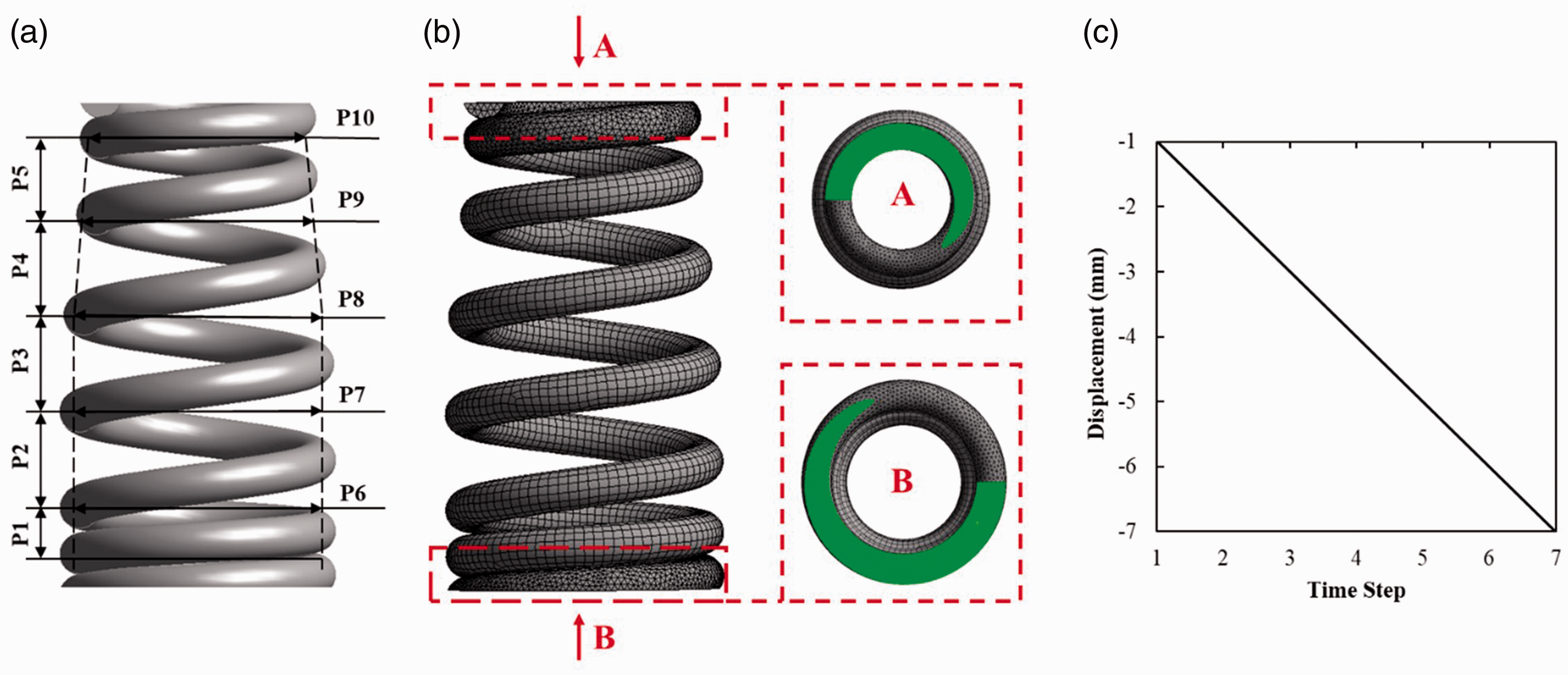
The geometry model of the beehive spring along with 10 defined variables (a) The meshing strategy (b) and boundary conditions of the FE model (c) The static 7 mm compression loading.

Table 1.

Mesh sensitivity analysis of the developed FE spring model.

Element size (mm)	0.8	1	1.2	1.4
Spring force at 7 mm (N)	312.65	312.09	312.02	311.5
Natural frequency (Hz)	540.72	540.28	540.58	540.79

Two types of analysis, static and modal analysis, are conducted using the FE model. In the static analysis, the spring is subjected to a static compressive loading from 0 mm to 7 mm (Figure 3(c)). The displacement input is applied on the upper end face A of the coil 07, while all degree of freedoms of the lower end face B of coil 01 are all constrained (Figure 3(b)). The reaction forces generated on the end face B are calculated. The self-contact between spring coils is defined in the model which allows the consideration of the non-linear effects caused by the coil clash during the spring compression. For the modal analysis, both end faces A and B of the spring are fixed at its free length (0 mm spring compression). The output is the first order natural frequency of the spring along the direction of the spring height. In Ansys Workbench, the modal analysis does not include the effects of self-contact between coils during vibration. However, the contact during the modal analysis is not significant according to the observation, because the spring is not compressed at free length.

Constrained Latin hypercube sampling (cLHS)

To analyse the interactional effects of the design parameters, a parametrical analysis is conducted using the developed FE model. The ranges of the 10 design parameters are listed in Table 2 together with their values of the benchmark beehive spring. As the investigated springs are always closed at both ends, the pitches of coil 01 and coil 07 are constants and are both 3.85 mm. Besides, a valve spring should be fitted into valve trains so that the diameters of coil 01 and coil 07 are also constants, which are 11.075 mm and 9.125 mm, respectively. These constrained lower and upper bounds of the parameters are determined according to the design specifications of the valve train of a real engine.

Table 2.

The ranges of the 10 design parameters.

Name	Lower bound	Upper bound	Default value (beehive spring)	Parameter
P1	4	6	5.419	Pitch of Coil 02
P2	7.5	9.5	8.777	Pitch of Coil 03
P3	7.5	9.5	8.817	Pitch of Coil 04
P4	7.5	9.5	8.622	Pitch of Coil 05
P5	6.5	8.5	7.64	Pitch of Coil 06
P6	9	12	11.075	Diameter of Coil 02
P7	9	12	11.075	Diameter of Coil 03
P8	9	12	11.075	Diameter of Coil 04
P9	9	12	9.5085	Diameter of Coil 05
P10	9	12	9.1725	Diameter of Coil 06

To generate different types of spring geometries for FE analysis, Latin Hypercube Sampling (LHS) method is used to determine the design parameters within the variable ranges (Table 2). LHS method is initially derived from the idea of a Latin Square (LS). Comparing to the conventional sampling method, such as Monte Carlo Sampling (MCS), the LHS generates samples evenly distributed in a 2D space (Figure 5(b)). It has shown superior efficiency compared to MCS when brought into line with finite element analysis.^21,22 The MCS samples, however, are randomly selected within the ranges of variables (Figure 5(a)), which may contain poor sampling areas.²³

The process of LHS is as following^24,25:

Divide evenly the range of each variable x_i into n intervals u_ij, i = 1, 2,…, r and j = 1, 2,…, n.

Calculate the cumulative probability of the j th interval of variable x_i as:

P_{i j} = \frac{(j - 1) + r_{i j}}{n}

Calculate the sample value x_ij by the inverse of the distribution function F(·):

x_{i j} = F_{i}^{- 1} (P_{i j})

Pair the values of each variable x_i with those of other variables randomly or in certain orders.

According to the principle of LHS method, the values of the design variables are determined within the defined ranges as shown in Table 2. However, some combinations of the selected values may not be rational in a practice design, which should be avoided in the analysis. In the case of the helical springs design, spring geometries such as the ones shown in Figure 4(a) are not desired according to the experience of spring designers. Since the sudden changes of the coil diameters can usually introduce high stress in these areas, pre-failure of a springs may occur. On the contrary, the spring such as the one shown in Figure 4(b), which has a progressive change on the coil diameters, is usually acceptable in practice. Therefore, it is essential to impose necessary constraints on the design parameters, so that only desired spring shapes can be generated.

Figure 4.

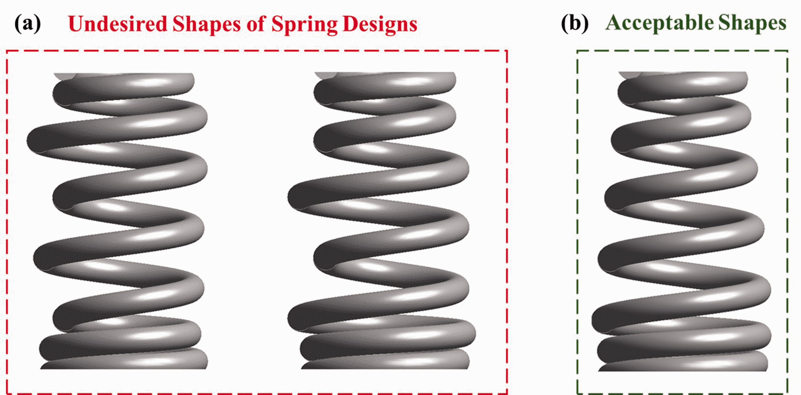
The samples of spring designs with (a) undesired shapes (b) acceptable shapes.

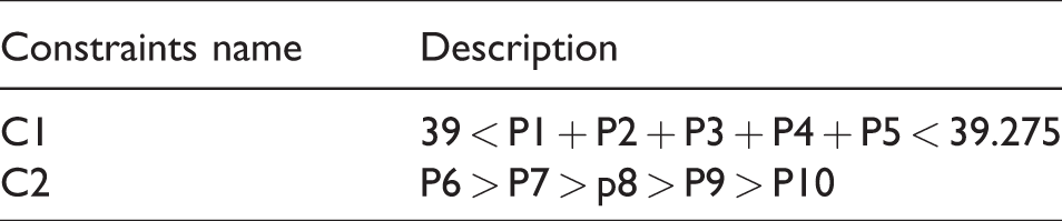
The method for achieving this goal is to apply constrained Latin hypercube sampling (cLHS) technique. The method is able to search a design space, which satisfy inequality constraints among the design parameters. As an extension of the conventional LHS, cLHS is a stratified sampling technique that can generate sample points more evenly than the constrained random sampling does.²⁶ As an illustration, Figure 5 shows 20 samples of two variables obtained from normal random sampling (Figure 5(a)), normal LHS (Figure 5(b)), constrained random sampling (Figure 5(c)) and cLHS (Figure 5(d)), respectively. In these figures, all the samples are selected with the x and y variables ranged within [0, 100]. Both the x and y axes are evenly divided into 10 intervals. The side bars of each scatter charts shown the quantities of the samples locating at each of these intervals. It shows that cLHS can generate even distribution of samples in every interval with the presence of inequality constraints. In this paper, cLHS is implemented to generate samples from the design domain defined by the variable ranges shown in Table 2. The inequality constraints defined for the valve spring designs are shown in Table 3. Constraint C1 means that only the spring samples that have desired spring height are selected. As a result, all the spring samples have similar spring lengths in a range of [45.5, 45.775], so they can be fit in the practical valve train. Constraint C2 shows that the coil diameters from coil 01 to coil 07 must be progressive. Based on the constraints, a number of 300 spring geometry models are generated from the design domain. These models are then imported to the FE simulation model to calculate static spring forces and natural frequencies.

Figure 5.

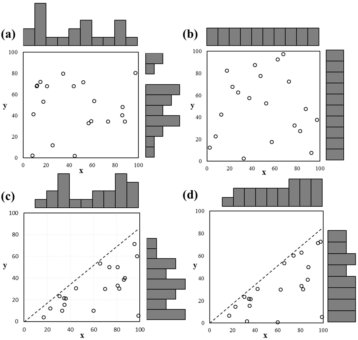
Samples of design of experiments (20 points) generated by (a) normal random sampling (b) normal Latin Hypercube sampling (c) constrained random sampling (d) constrained Latin Hypercube sampling.

Table 3.

Constraints on the design domain by inequalities of design parameters.

Constraints name	Description
C1	39 < P1 + P2 + P3 + P4 + P5 < 39.275
C2	P6 > P7 > p8 > P9 > P10

Genetic programming

Genetic programming (GP) is usually treated as a variant of genetic algorithm (GA), which applies the GA to a population of computer programs. GA is inspired by the Darwin’s theory of natural selection, and firstly proposed by john Holland in 1960. It was then continuously developed and extended by many other researchers to the present. A typical flowchart of the genetic algorithm is shown in Figure 6. Implementation of GA always starts with the generation of initial population. According to the principles of ‘survival of the fittest’, then, the fittest generation become the parent generations. The individuals of the parent generations evolve by going through the processes of selection, crossover, and mutation to generate children generations. The fitness of the children generation is also evaluated and the individuals with better fitness are stored for the next evolution. This process ensures that the most environmentally adaptive population can be evolved. At the end, the optimal individuals can be approximated as the optimal solution for the objective functions.

Figure 6.

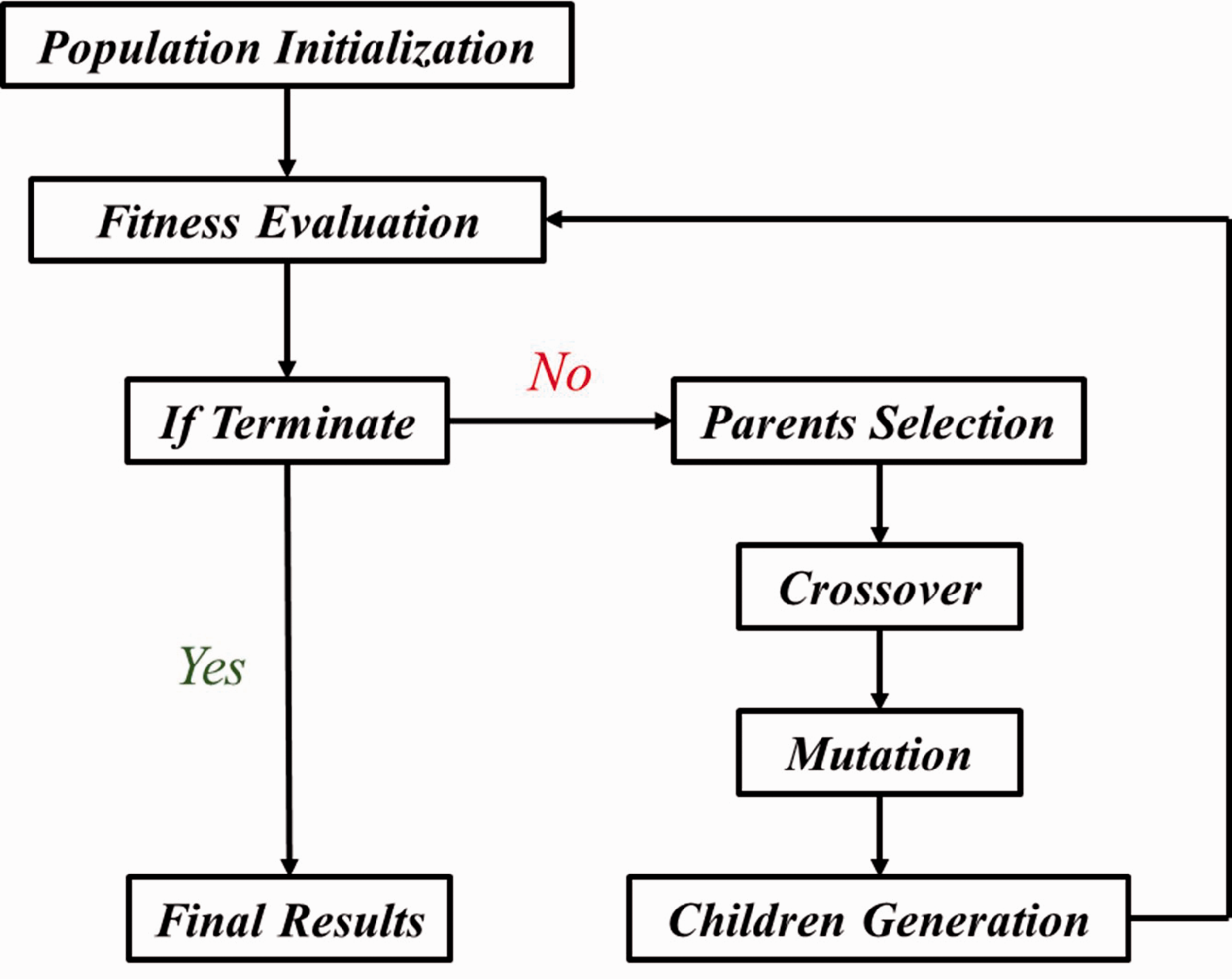
The flowchart for the main process of the genetic algorithm.

To apply the principles of GA to computer programs, GP adopts binary trees with branches and leaves to represent computer programs. It aims to evolve the computer programs to match as closely as possible to the desired goals. For example, the function of equation (4) is a desired goal to approximate.

y = 3 X_{1} - (2 - X_{0})

(4)

Firstly, GP starts with initializing the population of randomly developed binary trees consist of functions and terminals. Functions denote the operators in equations and terminals are the end nodes of these trees. Then, the fitness of every single tree is evaluated to determine if there is any meeting the terminate conditions. If not, these trees turn to be the parents’ generation to go through the crossover and mutation procedures. The crossover operates by randomly cutting two points from two trees and swap the cut portions to produce crossover offspring (Figure 7(a)). To avoid trapping in a local optimum, GP employs the mutation process. Figure 7(b) shows an example to conduct point mutation by selecting a random node and replacing it by another random one. Sub-tree mutation is based on the same logic, but it selects and replaces a random subtree instead of a random node. Consequently, GP accumulates these offspring of parent binary trees to form the new children generation. The fitness of every individual in the children generation should be evaluated. The children generation will then become the next parent generation to go through the procedures of crossover and mutation. The iteration process can always enhance the average fitness of every generation. The fitness of every individual in the children generation should be evaluated. Usually, a stop criterion is defined to stop the iterations. The best individual from the final generation provided by GP can be a solution for the researched problem.

Figure 7.

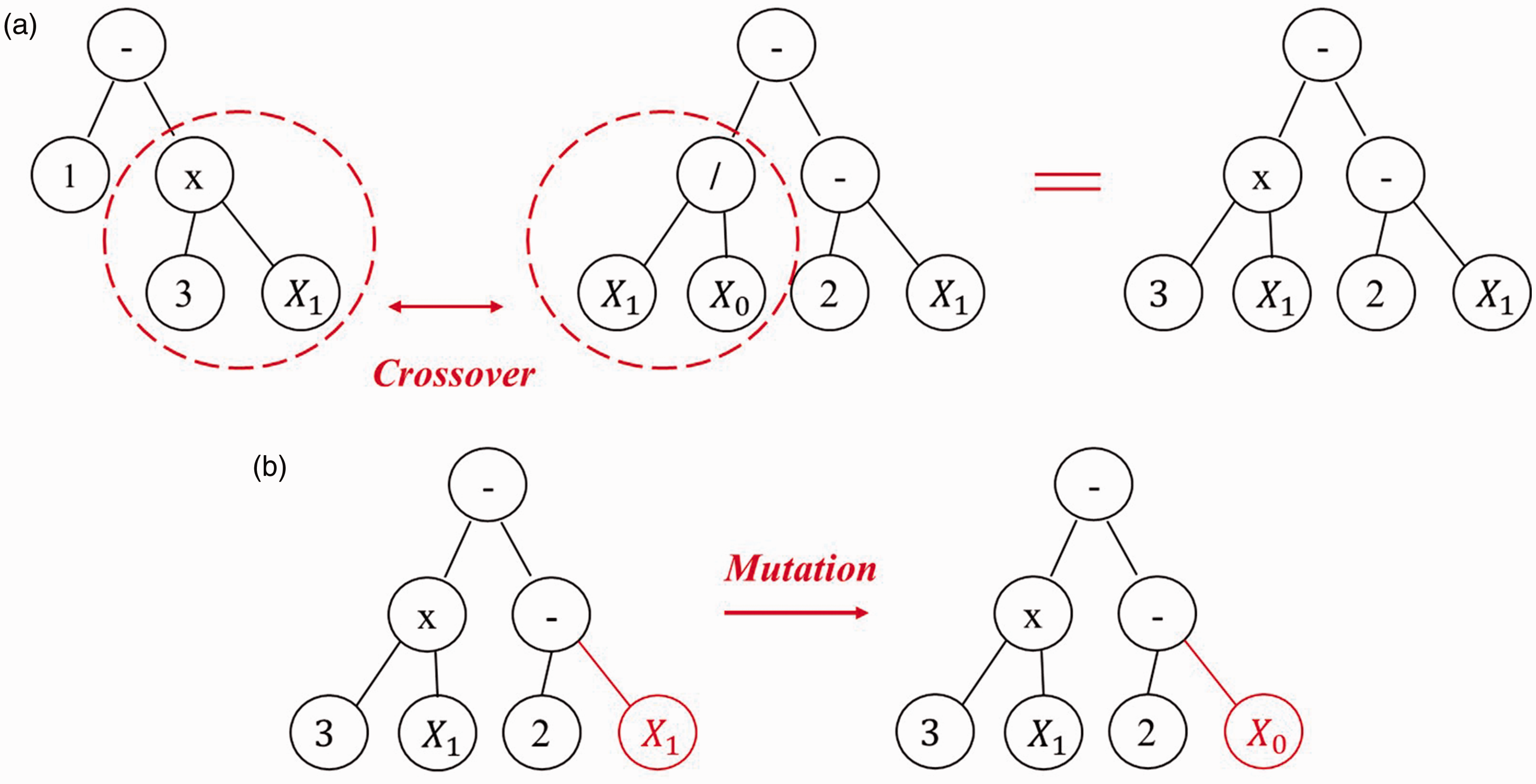
Schematic of methods used in GP during producing children generations: (a) Crossover (b) Mutation for Equation 4.

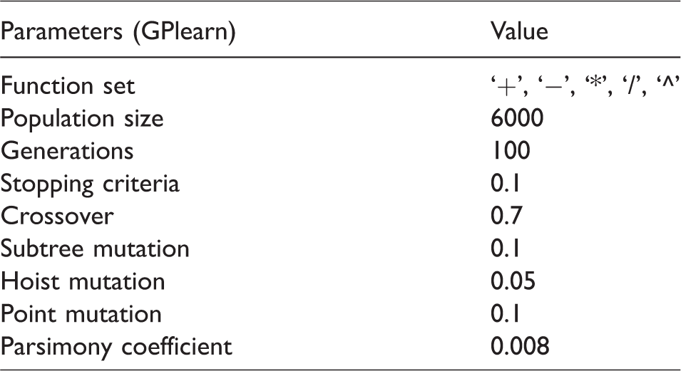
In this study, GP technique is employed to estimate the relationships between the parameters of the spring (Table 2) and the static compression forces applied on the spring. The Python machine learning package ‘GPlearn’ is used to program the GP algorithm. In total, 300 sets of parameters are selected by the cLHS method. Their corresponding FE simulation results are used to train and test the GP model. 250 sets of the FE results are used as training data and the other 50 sets are used as testing data. The parameters for developing the GP model are listed in Table 4. In the table, the population size is used to initial the structure of the GP program. The GP program solves for the desired solution and stops only when either the generations exceed 100 or the fitness is already lower than the stopping criteria 0.1. The parsimony coefficient is 0.008 in order to control the increasing size of the programs.

Table 4.

The parameters used for developing the GP model in ‘GPlearn’.

Parameters (GPlearn)	Value
Function set	‘+’, ‘−’, ‘*’, ‘/’, ‘^’
Population size	6000
Generations	100
Stopping criteria	0.1
Crossover	0.7
Subtree mutation	0.1
Hoist mutation	0.05
Point mutation	0.1
Parsimony coefficient	0.008

Results and discussion

Results and validation of FE and analytical analyses

Figure 8 shows the force-displacement relationships of the beehive spring obtained from the FE simulation, the analytical equation equation (1) and compression tests. The compression test on the beehive spring is conducted in the lab of Force Technology Ltd as shown in Figure 9(a). It shows that the result of the FE model has a good agreement with the experimental result. The stiffness calculated from the FE model k_FE is 44.58 N/mm at 7 mm compression, and the value based on the experimental result k_Exp is around 44.33 N/mm. On the contrary, the stiffness obtained from the analytical model has a constant value of 31.57 N/mm in the process of compression, which makes the force of spring around 91 N smaller at 7 mm compression than the one from the FE model and the experimental data. This difference is caused by the lack of considerations of coils contact in the analytical model.

Figure 8.

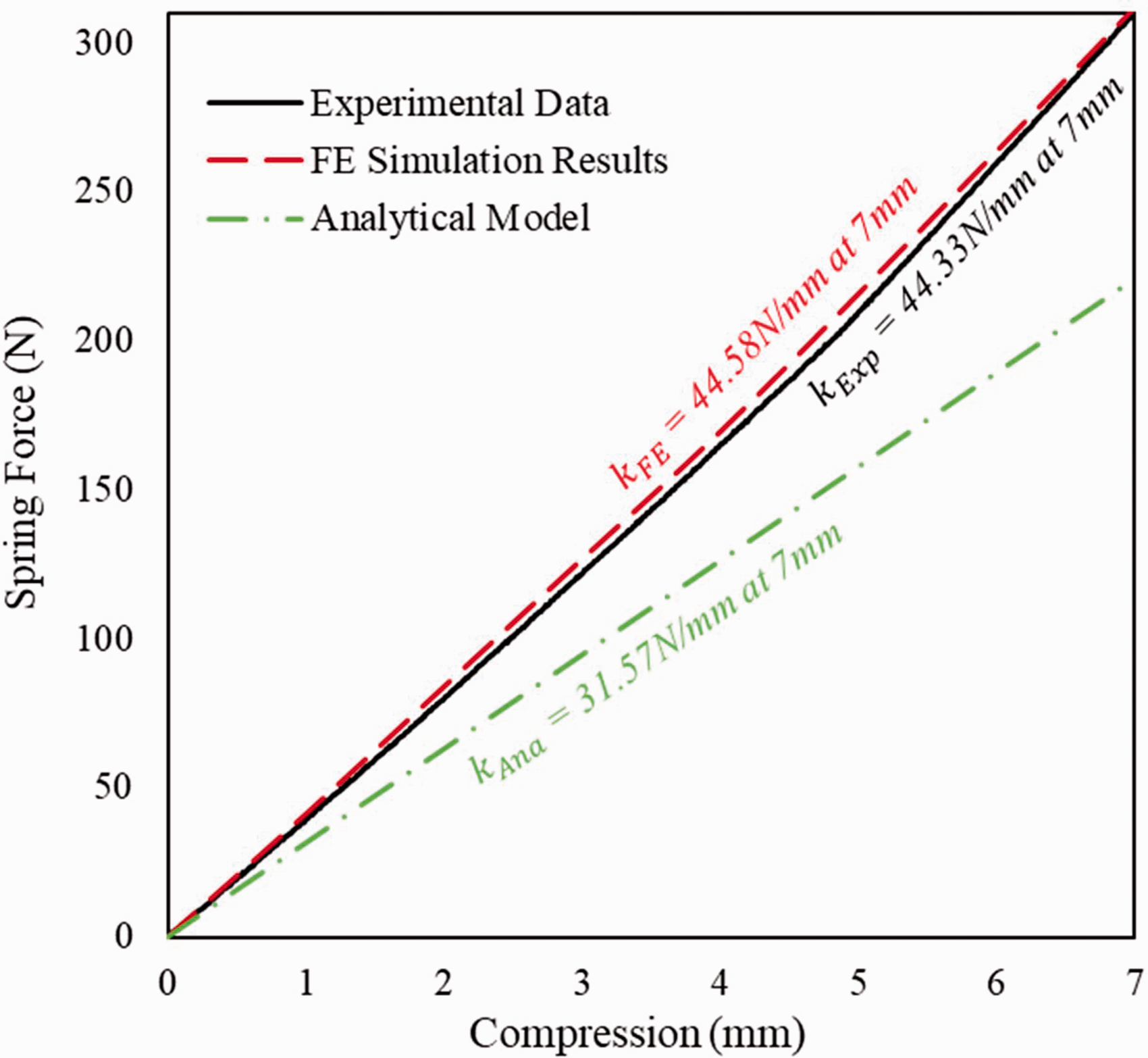
The spring compression results of the FE model, the analytical model and the exprimental test.

Figure 9.

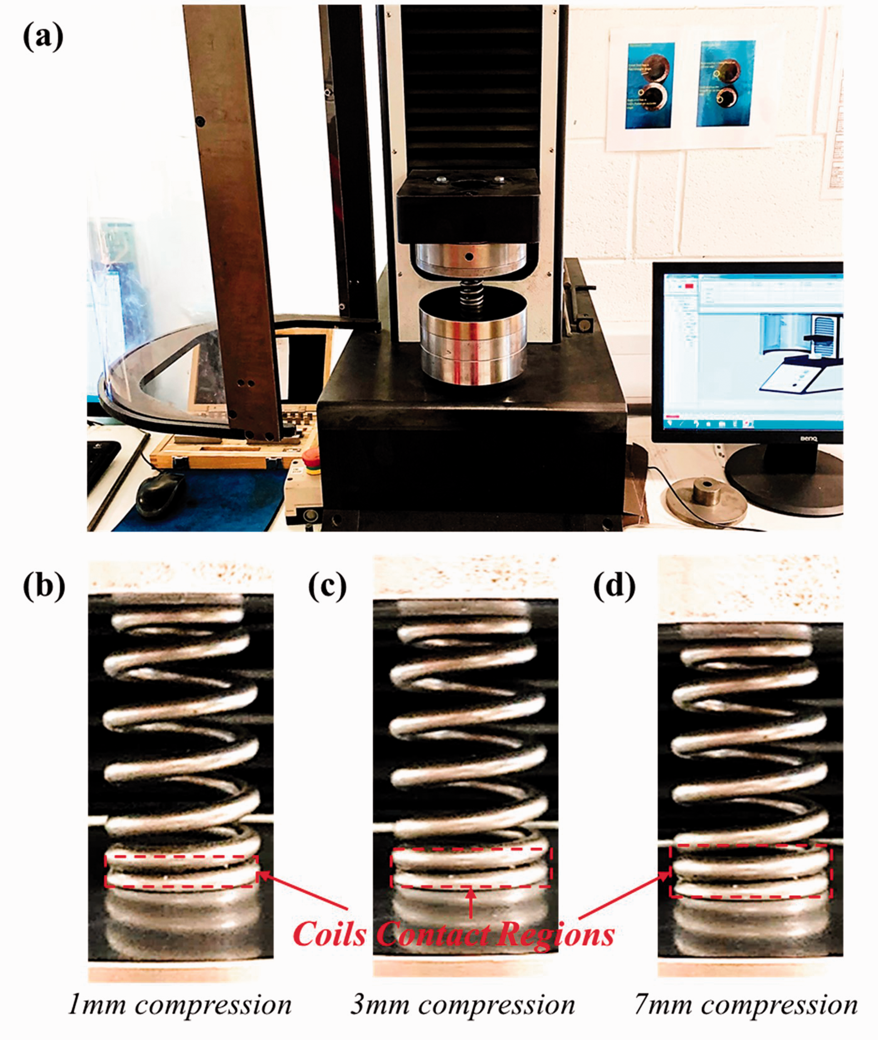
(a) The 7 mm compression test conducted on the beehive valve spring sample, and the contact status of spring coils at (b) 1 mm, (c) 3 mm and (d) 7 mm compression obtained from the testing result.

The coil contact regions of the spring at 1 mm, 3 mm and 7 mm compressions of the testing results are shown in Figure 9(b) to (d), respectively. It can be seen that the coil contact region is progressively increasing during the 7 mm compression. The coils contact regions at 1 mm compression (Figure 10(a)), at 3 mm compression (Figure 10(b)) and at 7 mm compression (Figure 10(c)) obtained from the FE simulation are shown in Figure 10. Both the results show that the lowest 2 coils (coil 01 and 02) are initially separated at free length and then starts to contact to each other at 1 mm compression. As a result, the gradients of the force curves in Figure 8 are close to each other before 1 mm compression. Then, the contact region begins growing due to the further compression. The contact regions of the test and the FE results at 3 mm compression is shown in Figure 9(c) and Figure 10(b). This process results in that the spring forces of the test result and the FE result increase more sharply than that calculated by the analytical model (Figure 8). The contact region keeps growing as the spring is continuously compressed, until the lowest 2 coils are fully contacted with each other at 7 mm compression (Figures 9(d) and Figure 10(c)). In practice, the increase of contact region reduces the number of active coils (Na), which, consequently, increases the stiffness of the spring. Therefore, the FE model which involves the effects of coils contact provides closer results to the experimental data. On the contrary, the traditional analytical model that is unable to capture coils contact is not accurate in simulating a spring having narrow pitch, where coils contact is likely to occur.

Figure 10.

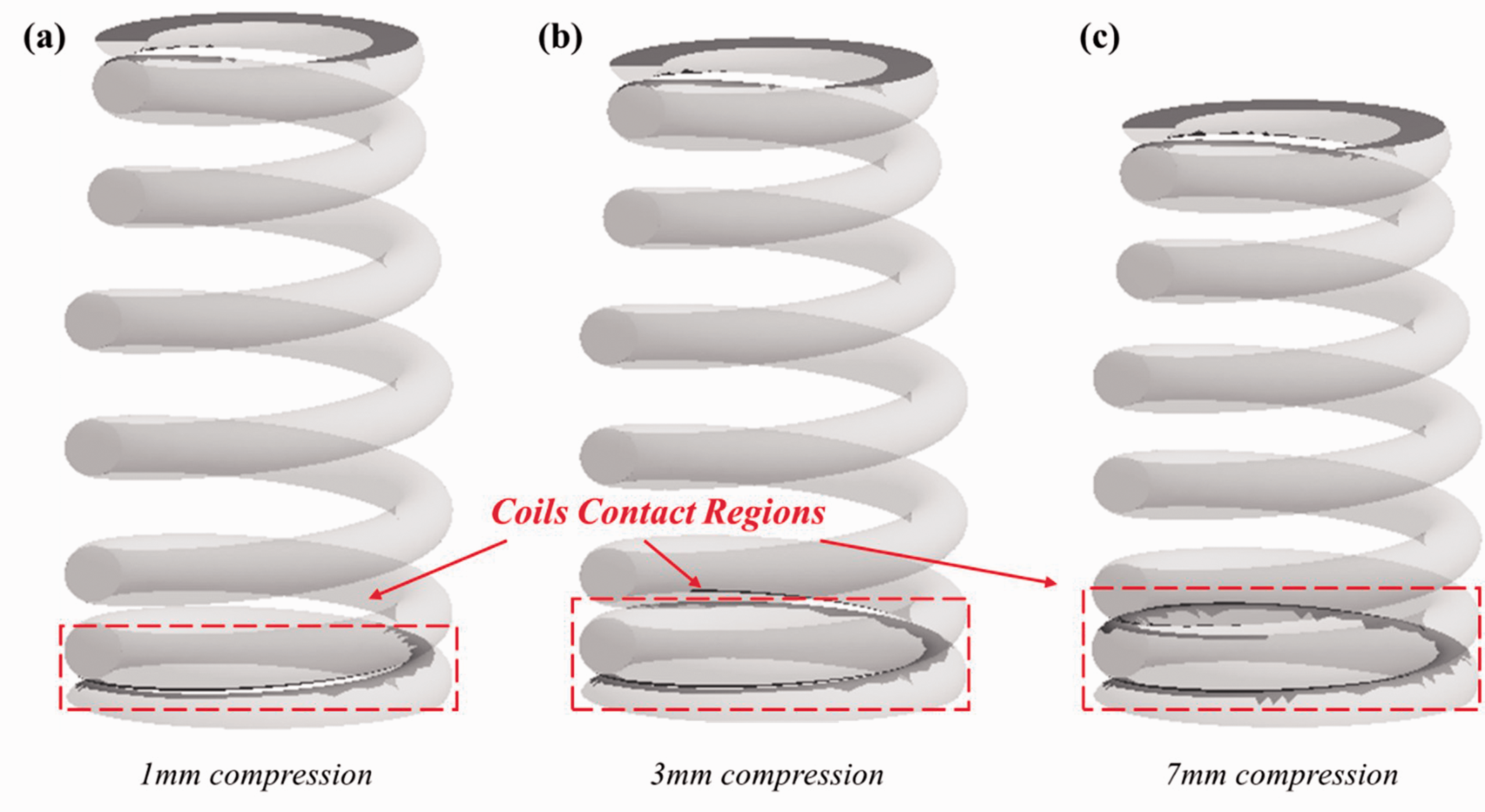
Contact status of spring coils at (a) 1 mm, (b) 3 mm and (c) 7 mm compressions obtained from the FE results.

GP analysis

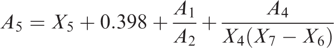
By adopting the GPlearn package and using the parameters defined in Table 4, an explicit expression for describing the relationships between the spring parameters (P1-P10) and the compression force F is generated as shown below: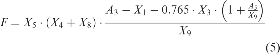

F = X_{5} \cdot (X_{4} + X_{8}) \cdot \frac{A_{3} - X_{1} - 0.765 \cdot X_{3} \cdot (1 + \frac{A_{5}}{X_{9}})}{X_{9}}

(5)

where

A_{1} = X_{4} - 2 X_{5} + X_{7} + \sqrt{X_{3} X_{8}} - 0.398

A_{2} = 2 X_{2} + X_{5} - X_{7} + 0.398

A_{3} = 2 X_{4} + X_{5} - X_{6} + 3 X_{7} + 2 X_{8} - X_{10} + 1.53

A_{4} = 2 X_{2} + X_{5} - \sqrt{X_{6}} \cdot (X_{8} - X_{2})

A_{5} = X_{5} + 0.398 + \frac{A_{1}}{A_{2}} + \frac{A_{4}}{X_{4} (X_{7} - X_{6})}

In addition, another explicit expression for describing the relationships between the spring parameters (P1- P10) and the first order natural frequency NF is modelled as shown below: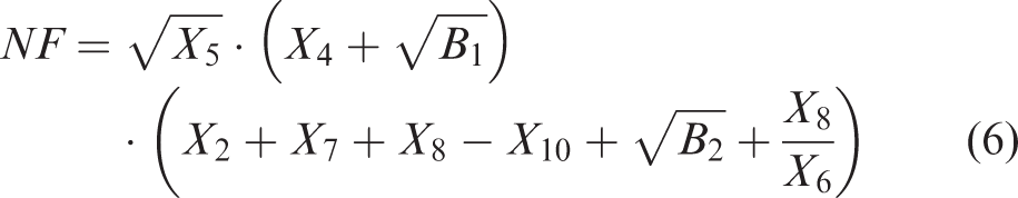

N F = \sqrt{X_{5}} \cdot (X_{4} + \sqrt{B_{1}}) \cdot (X_{2} + X_{7} + X_{8} - X_{10} + \sqrt{B_{2}} + \frac{X_{8}}{X_{6}})

(6)

where

B_{1} = X_{5} - X_{1} - X_{6} + X_{7} + X_{8} + X_{10} - 0.733 - \frac{X_{3}}{\sqrt{X_{2}}}

B_{2} = X_{2} - X_{1} - X_{6} + X_{5} + \sqrt{X_{7}} + X_{8} - X_{9} + X_{10} - 0.733 - \frac{X_{3}}{\sqrt{X_{2}}}

In these two meta-models, the ten variables X0–X9 represent for the 10 selected parameters of the beehive spring P1–P10 (Table 2). The correlation between the training data of spring forces and the results calculated by the GP model are illustrated in Figure 11(a). A large portion of the training data concentrates in the area where the spring forces stay between 240 N and 400 N. A same trend can be observed in the correlation between the spring force predicated by GP and the testing data as shown in Figure 11(b). Although most of the testing data stay in this area where spring force is lower than 400 N, the trained GP model is still able to predict the spring force that is larger than 400 N. Therefore, it can be concluded that the developed GP model is trained well to fit the data obtained from the FE simulations, and it shows a high accuracy in predicting the compression force.

Figure 11.

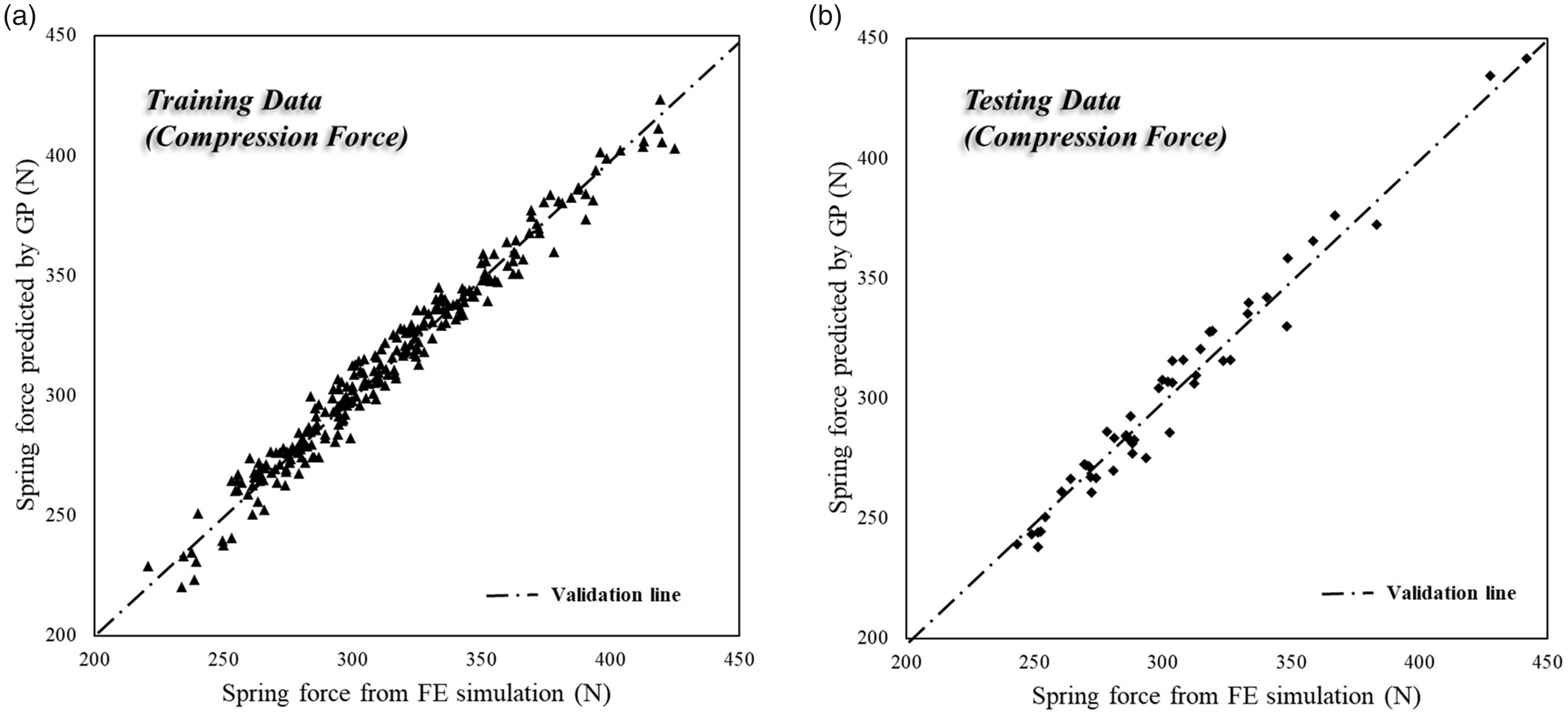
The correlations between the spring forces obtained by the FE simualtion and predicted by the GP model of (a) training data (b) testing data.

The correlation between the training data of first order natural frequency and the results obtained by the GP model are illustrated in Figure 12. As shown in Figure 12(a), the training data distributes evenly in the whole area between 450 Hz and 600 Hz. The testing data in Figure 12(b) also distributes evenly in this whole area. It can be observed that both the training data and the testing data in Figure 12 stay very close to the validation line. It means that the expression trained by GP is well trained to fit the natural frequency results obtained from the FE simulations. The trained GP model can predict the 1st order natural frequency accurately when the values of the ten spring parameters are given.

Figure 12.

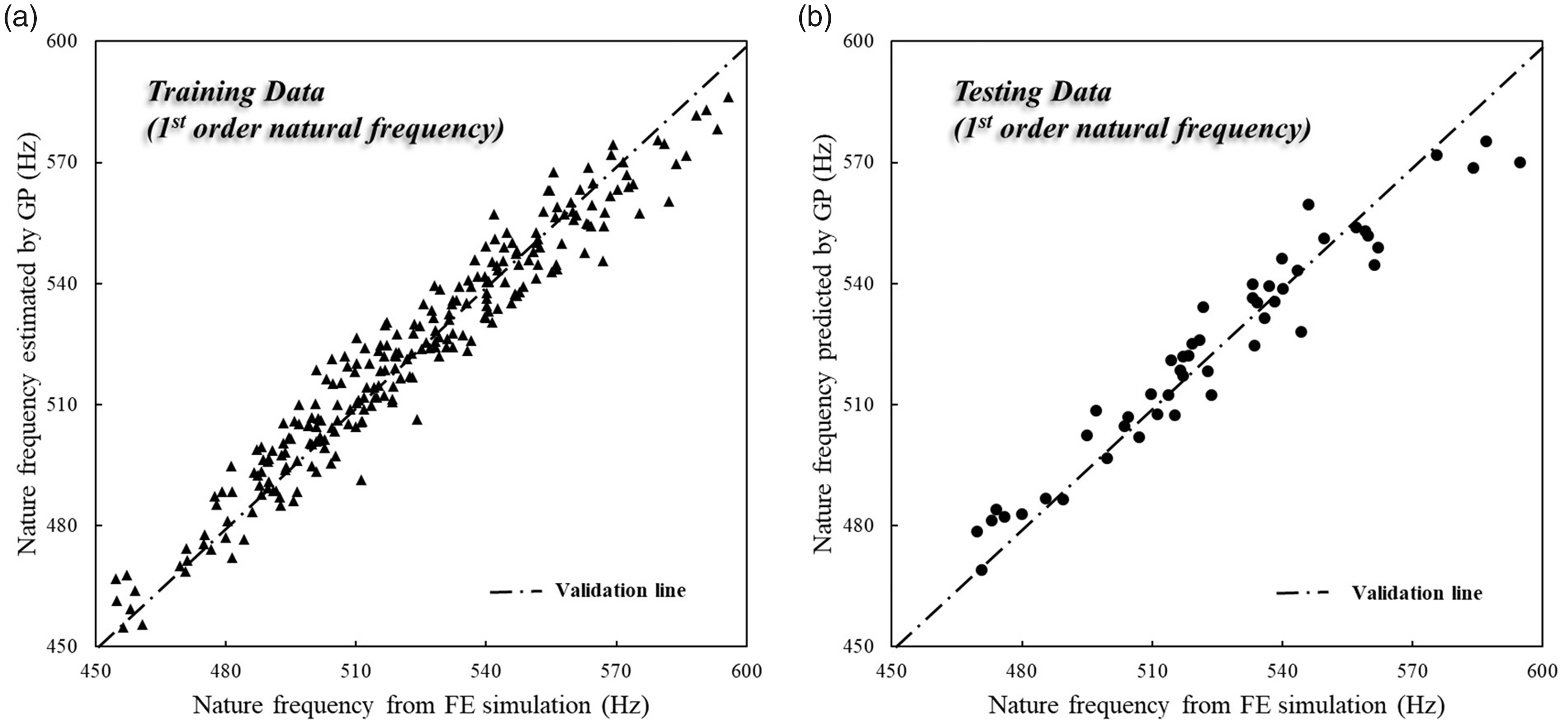
The correlations between the first order natural frequencies obtained by the FE simualtion and predicted by the GP model of (a) training data (b) testing data.

Sensitivity analysis of parameters

By employing the GP technique, the meta-models for predicting the compression force and the first order natural frequency of a helical spring are developed successfully. Then, a sensitivity analysis on the ten spring parameters can be conducted. To achieve this, the python package ‘SALib’ is used to implement the Sobol Sensitivity Analysis. The Sobol sensitivity analysis, or referred to as variance-based sensitivity analysis, is a method for analysing the global sensitivities of parameters. It is firstly proposed by Sobol²⁷ in 2001. In the analysis, the bounds for the ten parameters are defined by the same values as those defined in Table 2. Then, the sampler in the ‘SALib’ generates a certain number of samples for the analysis. The inherent function of the sampler for calculating the number of samples is N*(2D + 2), where N is the argument coefficient and D is the number of input parameters (D = 10 in this study). In the analysis, the argument coefficient N is assigned as 40,000 which makes the total number of samples is 8.8e5.

The sensitivities of the ten spring parameters to the compression force F is displayed in Figure 13(a). As defined in the previous section, the parameters P1–P5 represent the pitch of coils 02–06 and the parameters P6–P10 represent the diameters of coils 02–06. The sensitivities of parameters P2–P5 are generally higher than those of parameters P6–P10. It means that the value of the compression force is more sensitive to the changes in spring pitch than to the changes in the diameters of the coils. Theoretically, it is because that the changes of pitch determines the change of the number of active coils Na during a compression, which will significantly increase the compression force of a helical spring. It is noticed that the sensitivity of P1 is very small that has a value of 0.0004, which is attributed to the fact that the parameter P1, which represents the pitch of coil 02 (4–6 mm), is designed to be a damper pitch in the helical springs. This pitch is always smaller than the others (7.5–9 mm), which makes coil 01 and coil 02 constantly closed at 7 mm compression. Therefore, the variation of P1 does not affect significantly on the overall reaction force at 7 mm compression as it has nearly no contribution to the change of Na. Besides, it is observed that the sensitivity factor of P4 is 0.0093 in Figure 13(a), which is slightly lower than the factors of P2, P3 and P5. To verify this phenomenon, the displacements of coils 02–06 of the beehive spring at 7 mm compression are obtained as shown in Table 5. The displacements of coils 05 and 06 are smaller than those of coils 02, 03 and 04 due to the smaller coil diameters of coils 05 and 06, which is defined by as the cLHS approach. This should have made the sensitivities of P4 and P5 be lower than the those of P2 and P3. However, coil 06 is directly connected to the upper fixed end of spring, which means that it will contact the end of 07 progressively during compression. As a result, the closure between coil 06 and coil 07 makes the sensitivity factor of P5 (coil 06) stay high in Figure 13(a). Eventually, only the sensitivity of P4 (coil 05) is relatively small in Figure 13(a).

Figure 13.

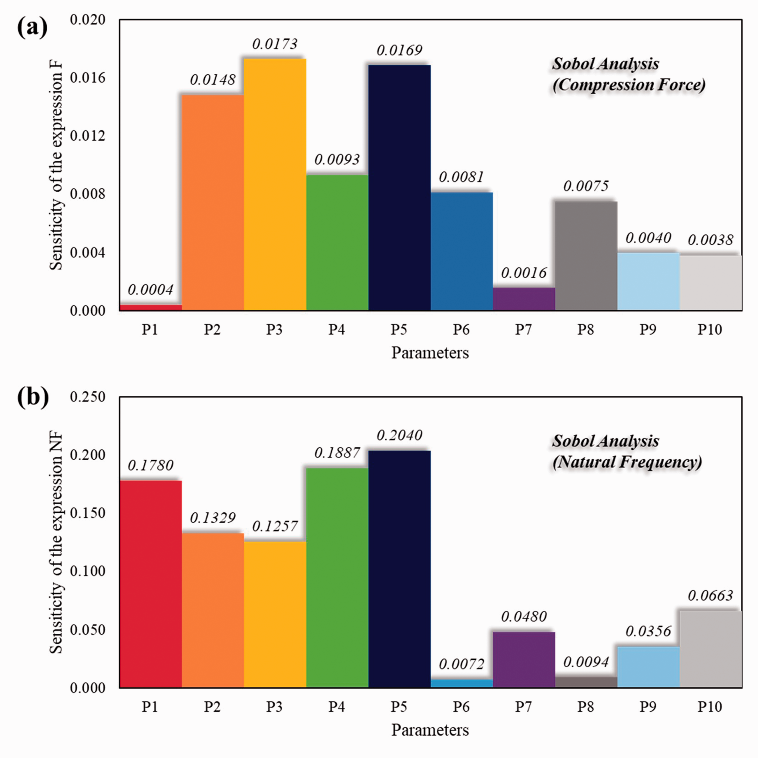
The sensitivities of spring parameters on th GP models for (a) the spring coompression force and (b) the first order natural frequency respectively.

Table 5.

The simulated displacements of coil 02–06 of the beehive springs at 7 mm compression.

Coil no.	02	03	04	05	06
Displacement (mm)	1.545	1.597	1.485	1.254	1.01

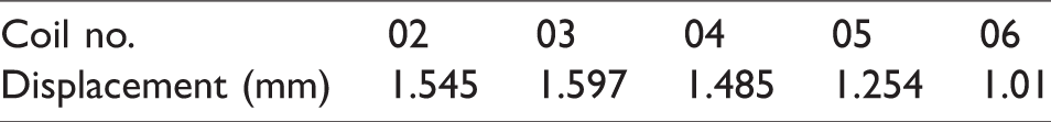
Figure 13(b) illustrates the parameter sensitivities to the first order natural frequency NF. The parameters P1–P5 show much higher sensitivities than those of the parameters P6–P10. It can be explained by that the changes of the spring pitches will alter the Na. At the free length, the change of Na has a significant effect on the result of the first order natural frequency.

In summary, the changes of spring pitches have more significant effects on both the results of the compression force and the first order natural frequency than the changes of coil diameters. However, the pitch of coil 02 (P1) has less effects on the force at 7 mm compression due to that the coil 01 and 02 are closed constantly.

Conclusion

In this article, an innovative study is conducted by combining the techniques of finite element analysis (FEA), constrained Latin Hypercube sampling (cLHS) and genetic programming (GP) to investigate the nonlinear relationships between design parameters and the mechanical properties of helical springs. The relationships between the spring parameters and the compression force and the natural frequency of helical springs with arbitrary shapes are successfully modelled for predicting the compression force and the natural frequency. The proposed method is proved to be a feasible and robust way to guide the design of helical springs of arbitrary shapes. The outcomes achieved by this study can be concluded as below.

Compared to the common LHS method, cLHS provides better flexibility and reliability in constraining an engineering design domain by defining inequalities between design parameters. It generates more representative samples for obtaining FE results and then used by GP model. The meta-models developed by GP describe the complicated relationships between the mechanical properties of helical springs and the multiple geometric parameters. It can also save a lot computational time by avoiding the time-consuming FE simulations. Besides, according to the results of sensitivity studies, it is found that though both the spring pitch and the coil diameter can affect the compressive force and the natural frequency of helical springs, the spring pitch has higher sensitivities than the coil diameter does. An exception is that when the spring pitch is too narrow, the pitch will be closed at a certain compression. Then, the sensitivity of that pitch to the compressive force becomes extremely small as it does not contribute to the change of the number of active coils at that compression. In addition, the results also demonstrate that the spring pitch and the spring diameter also contribute to the amplitude of spring force and natural frequency. The narrow pitch has significant effects on increasing the compression force as the coils having narrow pitch are closed progressively during compression.

In summary, cLHS is an outstanding candidate for engineering design sampling where predefined constraints exist. GP technique has a strong ability in conducting multi-parameters modelling and analysis. By combining the techniques of FEA, cLHS and GP, the present model shows its robust ability in design and analysis of mechanical devices with nonlinear programmed properties, which cannot be achieved by applying current existing methods of engineering design and analysis. The method also shows a big potential in aiding the process of engineering optimization by employing the meta-model in the future works.

Footnotes

Declaration of Conflicting Interests

The author(s) declared no potential conflicts of interest with respect to the research, authorship, and/or publication of this article.

Funding

The author(s) disclosed receipt of the following financial support for the research, authorship, and/or publication of this article: This work is funded by Lancaster University through European Regional Development Fund, Centre of Global Eco-Innovation, and industrial partners Force Technology Ltd.

ORCID iD

Zewen Gu

References

Pawar

Desale

Optimization of three wheeler front suspension coil spring. Procedia Manuf 2018; 20: 428–433.

Zhou

Chen

, et al. An enhanced flexible dynamic model and experimental verification for a valve train with clearance and multi-directional deformations. J Sound Vib 2017; 410: 249–268.

Guo

Zhang

, et al. Dynamic and exciting analysis with modal characteristics for valve train using a flexible model. Mech Mach Theory 2014; 78: 158–176.

Hou

Keating

, et al. Non-linear finite element model for dynamic analysis of high-speed valve train and coil collisions. Int J Mech Sci 2020; 173: 105476.

Wahl

AM.

Mechanical springs. New York: Penton Publishing Company, 1944.

Mancini

Piziali

Optimal design of helical springs by geometrical programming. Eng Optim 1976; 2: 73–81.

Muhr

TH.

New technologies for engine valve springs. SAE Trans 1993; 930912: 1336–1345.

Aurel

PS.

On the optimal design of helical springs of an automobile suspension. UPB Sci Bull Ser D 2009; 71: 81–94.

Pöllänen

Martikka

Optimal re-design of helical springs using fuzzy design and FEM. Adv Eng Softw 2010; 41: 410–414.

10.

Taktak

Omheni

Aloui

, et al. Dynamic optimization design of a cylindrical helical spring. Appl Acoust 2014; 77: 178–183.

11.

Zheng

Yan

, et al. Optimization design of the valve spring for abnormal noise control in a single-cylinder gasoline engine. Proc IMechE, Part D: J Automobile Engineering 2017; 231: 204–213.

12.

Qimin

Liwei

Qili

The optimal design and simulation of helical spring based on particle swarm algorithm and MATLAB. WSEAS Trans Circuits Syst 2009; 8: 84–93.

13.

Cramer NL. A representation for the adaptive generation of simple sequential programs. In: Proceedings of an international conference on genetic algorithms and the applications. Mahwah, New Jersey: Lawrence Erlbaum, 1985, pp.183–187.

14.

Yan

Cheng

, et al. Bi-directional prediction of structural characteristics and effective thermal conductivities of composite fuels through learning from finite element simulation results. Mater Des 2020; 189: 108483.

15.

Pala

Genetic programming-based formulation for distortional buckling stress of cold-formed steel members. J Constr Steel Res 2008; 64: 1495–1504.

16.

Beiki

Bashari

Majdi

Genetic programming approach for estimating the deformation modulus of rock mass using sensitivity analysis by neural network. Int J Rock Mech Mining Sci 2010; 47: 1091–1103.

17.

Cevik

Arslan

Köroğlu

MA.

Genetic-programming-based modeling of RC beam torsional strength. KSCE J Civ Eng 2010; 14: 371–384.

18.

Al-Mosawe

Kalfat

Al-Mahaidi

Strength of Cfrp-steel double strap joints under impact loads using genetic programming. Compos Struct 2017; 160: 1205–1211.

19.

Luo

Liu

Zhu

, et al. Metamodel-assisted design optimization of piezoelectric flex transducer for maximal bio-kinetic energy conversion. J Intell Mater Syst Struct 2017; 28: 2528–2538.

20.

Luo

Liu

Zhu

, et al. Maximum energy conversion from human motion using piezoelectric flex transducer: a multi-level surrogate modeling strategy. J Intell Mater Syst Struct 2018; 29: 3097–3107.

21.

Olsson

Sandberg

GE.

Latin hypercube sampling for stochastic finite element analysis. J Eng Mech 2002; 128: 121–125.

22.

Pahner

Mertens

De Gersem

, et al. A parametric finite element environment tuned for numerical optimization. IEEE Trans Magn 1998; 34: 2936–2939.

23.

Olsson

Sandberg

Dahlblom

On Latin hypercube sampling for structural reliability analysis. Struct Saf 2003; 25: 47–68.

24.

Stein

Large sample properties of simulations using Latin hypercube sampling. Technometrics 1987; 29: 143–151.

25.

Minasny

McBratney

AB.

A conditioned Latin hypercube method for sampling in the presence of ancillary information. Comput Geosci 2006; 32: 1378–1388.

26.

Petelet

Iooss

Asserin

, et al. Latin hypercube sampling with inequality constraints. AStA Adv Stat Anal 2010; 94: 325–339.

27.

Sobol

IM.

Global sensitivity indices for nonlinear mathematical models and their Monte Carlo estimates. Math Comput Simul 2001; 55: 271–280.