
Abstract
This paper discusses cooperative path-planning and tracking controller for autonomous vehicles using a distributed model predictive control approach. Mixed-integer quadratic programming approach is used for optimal trajectory generation using a linear model predictive control for path-tracking. Cooperative behaviour is introduced by broadcasting the planned trajectories of two connected automated vehicles. The controller generates steering and torque inputs. The steering and drive motor actuator constraints are incorporated in the control law. Computational simulations are performed to evaluate the controller for vehicle models of varying complexities. A 12-degrees-of-freedom vehicle model is developed and is subsequently linearised to be used as the plant model for the linearised model predictive control-based tracking controller. The model behaviour is compared against the kinematic, bicycle and the sophisticated high-fidelity multi-body dynamics CarSim model of the vehicle. Vehicle trajectories used for tracking are longitudinal and lateral positions, velocities and yaw rate. A cooperative obstacle avoidance manoeuvre is performed at different speeds using a co-simulation between the controller model in Simulink and the high-fidelity vehicle model in CarSim. The simulation results demonstrate the effectiveness of the proposed method.
Keywords
Introduction
The main components of an autonomous vehicle are perception, planning and control. This paper discusses the planning and control aspects. For collision avoidance, generally a hierarchical control scheme is used with high level path-planner 1 and low level tracking controller. 2
Significant research has been done in path-planning strategies using mixed-integer quadratic programming (MIQP), 3 polynomials, 4 B-splines, 5 elastic bands 6 and potential fields. 7 In the research community, the path-planning problem has been widely studied for a single vehicle while in an autonomous driving environment multiple vehicles are present. A challenging research task is to achieve coordination by considering the trajectories of other autonomous vehicles. Schouwenaars et al. 8 used an optimal path-planning approach for multiple vehicles based on MIQP. Frese and Beyerer 9 compared several cooperative path-planning algorithms like tree search, elastic bands, priority-based approach, etc. for their computational times.
The lower level path-tracking controller ensures that a collision-free path is generated while a successful obstacle avoidance manoeuvre is achieved by making the vehicle precisely follow the planned trajectory. Trajectory tracking methods use fuzzy logic, 10 proportional–integral–differential, 11 pure pursuit strategy, 12 linear quadratic regulator, 13 sliding-mode control, 14 robust control 15 and model predictive control. 16 MPC-based controllers easily handle actuator constraints and other uncertainties. 17
Tracking controller requires vehicle model for mapping the reference trajectories. Researchers have widely used simplified models like kinematic model, 18 bicycle model, 19 planar lateral dynamics full car model 20 and models ignoring effects of roll, pitch and heave motions for developing the tracking controller. 21 Moreover, when the chassis angular motions are considered, a general assumption is made that the vehicle rolls and pitches about the centre of gravity (CG), while in fact the vehicle rolls and pitches about roll and pitch axis respectively. 22 For low-speed manoeuvres, simplified models capture the vehicle dynamics characteristics sufficiently well but at higher vehicle speeds and limits of handling there are significant differences in the predictions of these simplified. 23 These models are routinely linearised about an operating point but they deviate significantly from the nonlinear models at other operating points. To overcome this limitation, some researchers have used linear time-varying bicycle model but effect of out-of-plane motions is not captured. 24 Our contribution in this direction is to develop a linear time-varying model that captures the coupling effects of roll, pitch and heave motions.
Moreover, the limitation of simplified models is that only a limited number of vehicle states can be controlled. A vehicle model of intermediate complexity between a sophisticated commercial multibody dynamics model 25 and these simplified vehicle models is desirable for a real-time application. We developed a four-wheel vehicle model considering the effects of roll, pitch and unsprung mass motions, which can emulate real vehicle dynamic characteristics with low computational expense.
The main contribution of this paper is to develop a cooperative path-planning and tracking algorithm and evaluate it using models of varying complexities.
The cooperative path-planning architecture is based on a distributed MPC approach, where path-planner for each vehicle optimises its optimal trajectory according to the planned trajectories of their neighbouring vehicles that is broadcasted at each time step. In the tracking controller, a future input sequence of steering angle and drive torque is calculated for a predefined prediction horizon. The vehicle trajectories that are tracked are the positions and velocities in longitudinal and lateral directions.
The paper is organised as follows: methodology is described at first followed by the vehicle dynamics model. Four different vehicle models, namely, the kinematic model, bicycle model, a 12-degrees-of freedom (dof) model of intermediate complexity and a high-fidelity CarSim model are discussed in the vehicle model section. A relative comparison study of the vehicle trajectories obtained from various vehicle models for a single lane change manoeuvre is performed. The nonlinear vehicle model is subsequently linearised to be used in the MPC formulation for tracking. Next, the path-planning algorithm developed using model predictive control and MIQP is discussed followed by the formulation of the tracking controller. The results are discussed for a cooperative double lane change manoeuvre and finally conclusions are discussed.
Methodology
The proposed hierarchical scheme is shown in Figure 1. On the upper level, given a set of vehicles Proposed algorithm of path planning and tracking.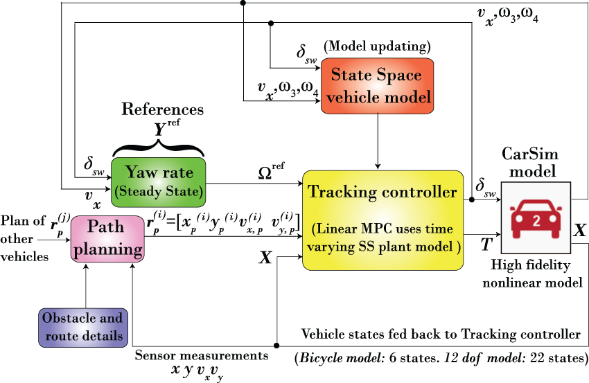
To generate the collision-free reference trajectories, we assume that at every time step k, each vehicle i receives the future plans of the others agents
On the lower level, the tracking controller tracks the trajectory (i.e. a set of way-points)
MPC-based path-tracking algorithm is presented to follow desired speeds while allowing to temporary deviate from desired paths in Funke et al.
26
The underlying idea of optimisation with both velocity and position states is quite useful.
27
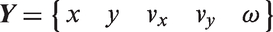
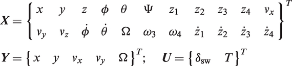
In addition to tracking of the longitudinal and lateral positions and velocities, we also track the yaw rate reference. Therefore, the vehicle control output vector is given by
Vehicle model
Four vehicle models are described in the following sections.
Kinematic model
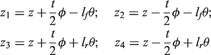
The kinematic vehicle model is shown in Figure 2(a). The inputs to the model are vehicle speed v and steering angle δ. From Figure 2(a), the longitudinal and lateral velocities of the centre of mass G are given by
(a) Kinematic model; (b) bicycle model.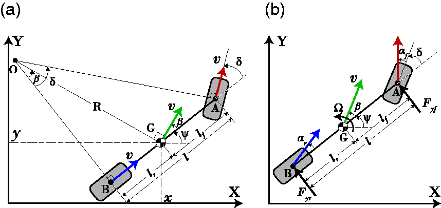

This model assumes no-slip condition. This implies that the velocities of each wheel points in the same direction of wheel and are equal. As there is no-slip condition, there lies an instantaneous centre of rotation ‘O’ about which the vehicle rotates and the rotation rate of the vehicle Ω is given by


From Figure 2(a)

Bicycle model
The bicycle model is shown in Figure 2(b).
Under small steering angle approximation, the front and rear slip angles are given by

The lateral acceleration of the CG a
y
can be obtained from the fixed and rotating coordinate system representation as

The lateral force balance equations for the bicycle model (again under small angle approximation) is given by

F
yf
and F
yr
are the front and rear cornering forces given by
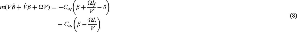
From equations (4), (6) and (7) we obtain

The longitudinal force balance (under small steering angle δ approximation) yields

F
d
is the aerodynamic drag and F
r
is the rolling resistance given by

C
d
is the drag coefficient, C
r
is the coefficient of rolling resistance, A is the car frontal area and W is the vehicle weight. For simplicity we assume no longitudinal slip, which implies that,
Finally, yaw moment balance about the CG ‘G’ yields

Equations (8) to (11) represent governing equations of motion.
12-dof model
The 12-dof model is shown in Figure 3.
12-degrees-of-freedom vehicle model.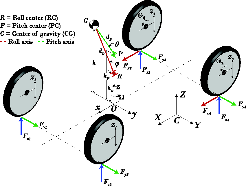
This model consists of three translational dof corresponding to longitudinal, lateral and vertical motion; three rotational dof corresponding to roll, pitch and yaw; four dof (one for each wheel) for wheel jounce; two dof for the angular rotation of rear left and right wheels. Note that in our present study, we have considered a vehicle with rear wheel drive and so we are interested only in the rear wheel velocities for longitudinal slip calculation as described in the section on the wheel model.
Coordinate system
It is convenient to write the equations of motion in noninertial (moving) reference frame Fixed and rotating coordinate systems.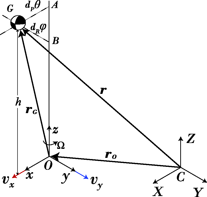
For deriving all equations of motion, small angle approximation for roll, pitch and wheel steering angle is considered. Eventually, the nonlinear equations of motion are linearised and are represented in the state-space form.
Planar motions
In this section, we study the planar motions of the chassis in x, y directions and yaw about z-axis.
The absolute position of the vehicle CG is given by

The position vector

Since

For small pitch and roll angles, above equation reduces to


Sum of the external forces is equal to the rate of change of linear momentum

For small values of wheel steering angle δ and side-slip angles α
i
, the equations can be linearised and the resultant forces in x and y directions are given by (There is a small difference between left and right wheel steering angles for normal handling situations. Using the same steering angle for both inner and outer wheels is an acceptable approximation for handling analyses.
29
)

It is important to note here that the vehicle used for this study has rear wheel drive and therefore the longitudinal forces are generated by rear tyres only (see Figure 3).
F
d
is the aerodynamic drag and
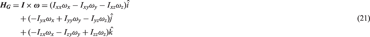
To study the yaw dynamics, we begin with the calculation of the angular momentum. The angular momentum

The elements I
xx
, I
yy
and I
zz
are the inertia moments and I
xy
, I
yz
and I
zx
are inertia products and are the off-diagonal terms of the inertia tensor. The components of the angular velocity

For calculating the angular momentum

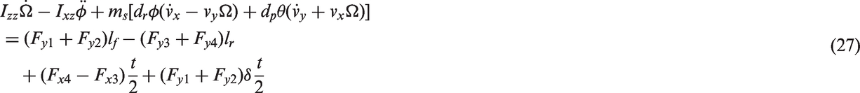
Finally the moment balance equation is given by

Considering the moment balance in z direction about O in Figure 5 we obtain
Lateral dynamics model.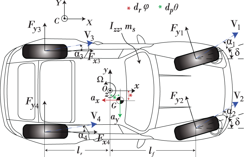

The external moment
It is important to note that the input given by the driver is the steering wheel angle

Finally, the in-plane motions can be studied using longitudinal and lateral force balance equations in (18) and yaw moment balance equation in (27).
Out-of-plane motions
In this section, out-of-plane motions: roll, pitch, heave and wheel jounce motions are analysed.
The vehicle rolls about the roll axis passing through the front and rear suspension roll centres.
30
The distance between the CG and the roll axis (roll centre) is the roll moment arm d
r
(see Figure 6). The roll centre height varies with suspension travel but for the sake of simplicity this variation is neglected.
Roll dynamics model.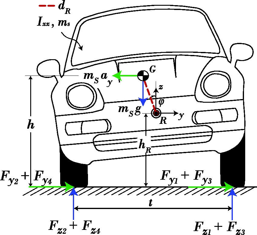
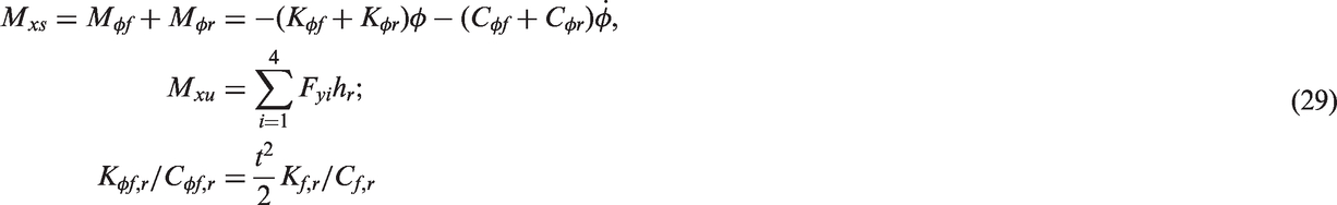
M
xs
and M
xu
are sprung mass and unsprung mass roll moments given by


As similar to the roll dynamics, the vehicle pitches about the pitch centre P in Figure 3. The distance between the CG and the pitch centre is the pitch moment arm d
p
(see Figure 7). Considering the pitch moment balance (small pitch angle approximation) about the pitch centre P we obtain
Pitch dynamics model.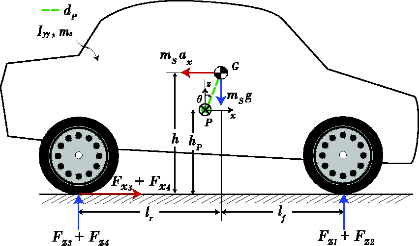

In this part, we will study the heave motions of the chassis and wheel jounce. To study this, we will consider the 7-dof ride model of the car as shown in Figure 8.
7-dof ride model. In the present study, the vehicle moves on a flat road so ground deflections are not considered.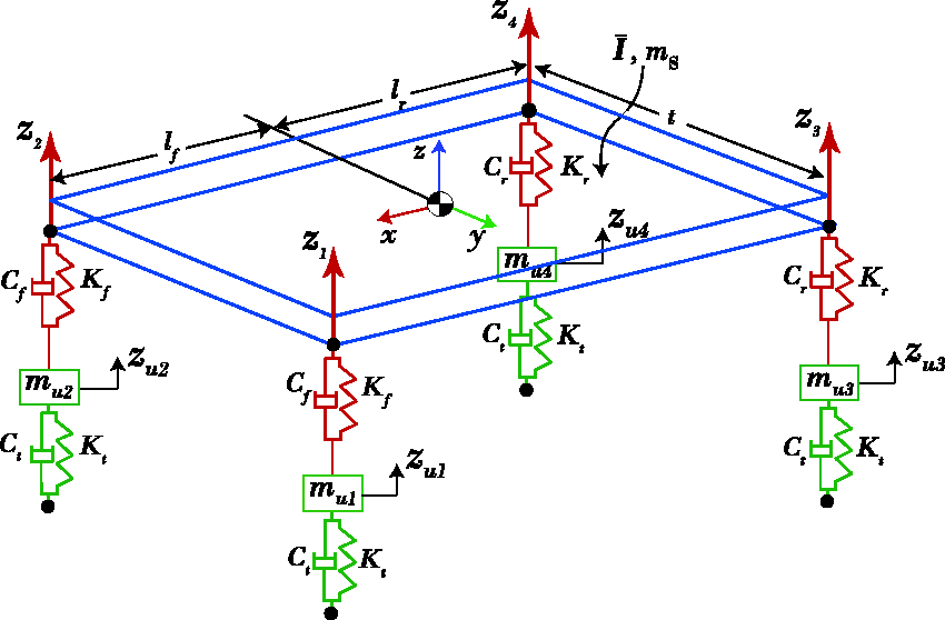
Considering the force balance in z direction, the governing equation for the chassis heave motion z is given by

Considering the force balance in z direction for each unsprung mass we obtain the wheel jounce z
ui
as

The vertical forces on the tyres is given by

The longitudinal and lateral forces are generated by the wheels. As pointed out earlier, we have considered a rear wheel driven vehicle. As a result, the longitudinal force is generated only by the rear wheels while the lateral forces are generated by all the four wheels.
The first step in calculating the forces generated by a tyre, is to compute the longitudinal slip s
xi
, and lateral slip s
yi
. To calculate wheel slip we require wheel corner velocities and wheel angular speeds, which are obtained from Figure 9.
(a) Corner velocities; (b) wheel angular dynamics.
The wheel corner velocities depend on vehicle velocity, yaw rate and geometrical parameters of the chassis as

The theoretical slip quantities are defined as
31

The overall or total slip at each tyre is defined by

Next the total friction coefficient using Pacejka's ‘magic formula (MF)’ is given by

Assuming symmetric tyre characteristics, the total friction force for each tyre lies within the friction circle and the longitudinal and lateral tyre forces are given by
32

In the above equations, the wheel angular velocity

In our case, the engine torque T is equally distributed to both the rear wheels as the vehicle considered for study is a rear wheel driven car with an open differential of gear ratio 1. As a result, only the longitudinal slips of rear wheels come into picture
In addition to these we have developed a sophisticated multi body dynamics vehicle model in CarSim which represents a real world vehicle and will be eventually used to evaluate the tracking controller.
The CarSim modeling interface is shown in Figure 10. The vehicle model was built for a prototype Westfield Sports Car.
33
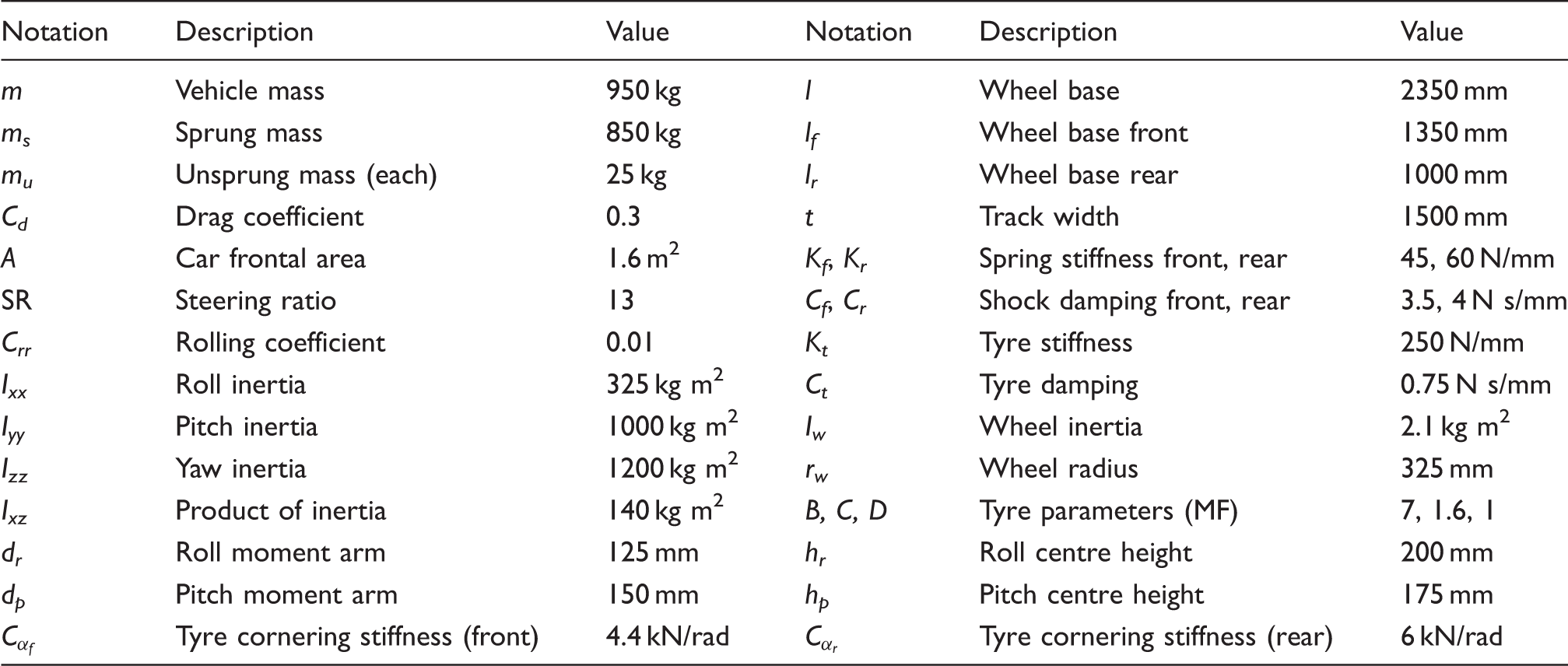
The weight, inertia, CG location of the vehicle, suspension and steering properties were obtained from measurements. The vehicle parameters used in this model are reported in Table 1. The vehicle is equipped with double wishbone suspensions in both front and rear axles with a rigid roll-cage chassis. The values for spring and damper parameters, roll centre height, track width, spin inertias and compliance coefficients were used to build the suspension model. The suspension kinematics and compliance characteristics were fed as look-up tables in CarSim to model the suspension characteristics. An approximate linear relationship between handwheel and roadwheel steer angle is found for the range of CarSim modeling interface. Vehicle parameters used to develop the mathematical model.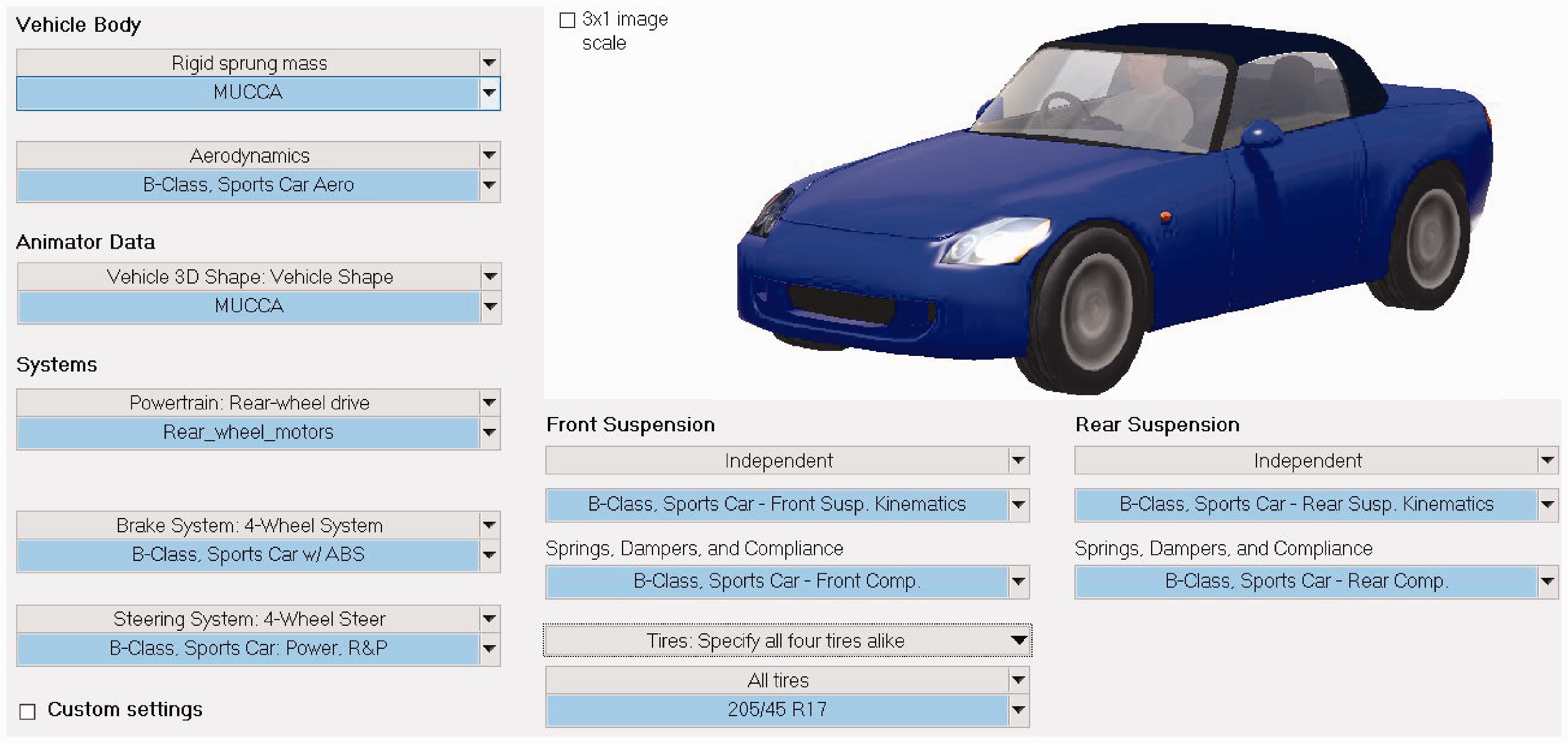
The mathematical model so developed has 57 dof, which in turn solves 114 first-order differential equations to calculate the vehicle responses. This model is exported as an S-function and in Simulink and a co-simulation interface is setup to assess the performance of the tracking controller.
Model comparisons
So far we developed four vehicle models, namely, kinematic model, bicycle model, 12-dof model and the CarSim model. These models differ from each other in terms of complexity. The kinematic model is the simplest with only three states. It does not take into account tyre compliance and is geometry based. The bicycle model is a further correction of the kinematic model with tyre lateral compliance taken into account. The 12-dof model takes suspension compliance, out-of-plane motions and wheel jounce into account and is a model of intermediate complexity as opposed to the sophisticated high-dof CarSim model.
The predictions of these vehicle models differ significantly at high lateral accelerations. To demonstrate this, the vehicle trajectories obtained from various models for a lane change manoeuvre at 80 km/h are compared in Figure 11. A sinusoidal steering wheel angle of 26 ° is given to achieve a lane change manoeuvre. The vehicle path X – Y, lateral velocity v
y
and yaw rate Ω trajectories are obtained for each model.
Responses of different models for a sinusoidal steering wheel angle input for a lane change maneuver at 80 km/h.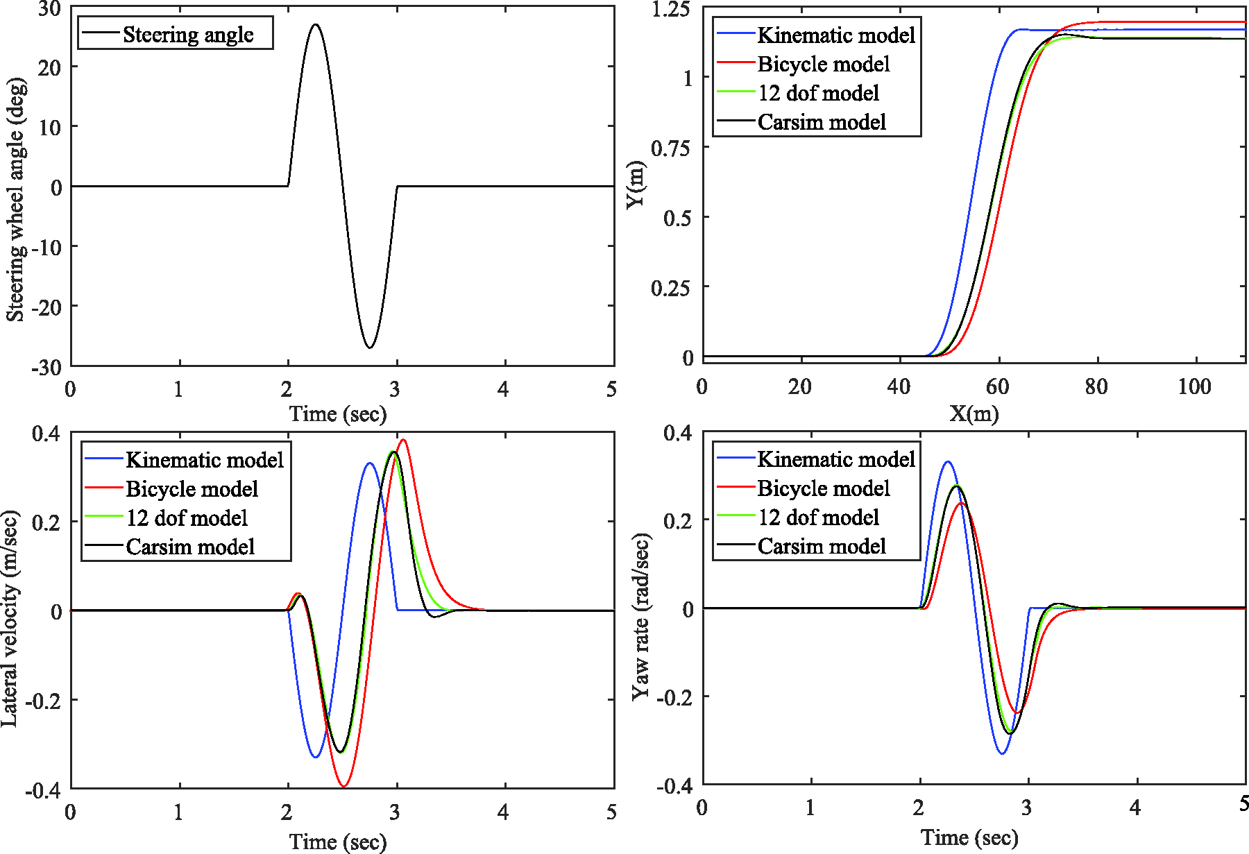
From Figure 11, it is evident that the predictions from Kinematic model substantially differ from that of the sophisticated CarSim model. Bicycle model gives a better prediction of the yaw rate response but it fails to give a representative prediction of lateral velocity and correspondingly the lateral position trajectories. The 12-dof proposed model is midway in complexity as opposed to the CarSim model and it fairly captures all the necessary vehicle dynamic handling characteristics.
For subsequent implementation, we have chosen 12-dof model and will compare its response against the bicycle model after integrating path-planning and tracking controller. Now, we discuss the linearisation of these models.
Linearisation
The governing equations of the vehicle dynamics model developed in the earlier section, can be written in first-order form as

Next, the above nonlinear model can be linearised by expanding around the equilibrium point (
The resultant linearised model is given by
For bicycle model, For 12-dof model


Output matrix, For bicycle model
For 12-dof model

The ground wheel angle δ is obtained by dividing the handwheel steering angle δ sw by the steering ratio (SR).
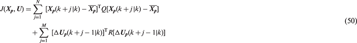
Finally, the state matrices are discretised to obtain a discrete time state-space model as

For bicycle model:
For 12-dof model:
These discrete time matrices are obtained using the zero-order hold (ZOH) discretisation method in Matlab, with an integration step of
Path-planning
The path-planner generates optimal trajectories using a mixed-integer quadratic programming approach with collision avoidance constraints in a receding-horizon fashion. 34
Collision avoidance
Collision avoidance between two autonomous vehicles is ensured by following linear inequality convex constraints
Big-M method is used to rewrite the collision avoidance constraints in terms of binary variables 
The binary variables
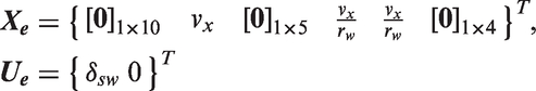
To achieve obstacle avoidance with static objects, we incorporate the same constraints set as described in equation (47) replacing the planned trajectories Remark 1
The location of the obstacles is known. This assumption can be satisfied by using cameras, for example light detection and ranging (LiDAR) system attached to the vehicle. 35
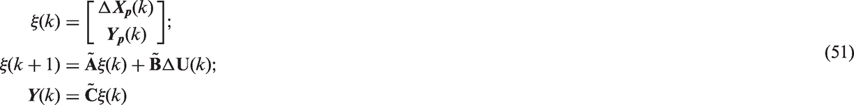
State-space model
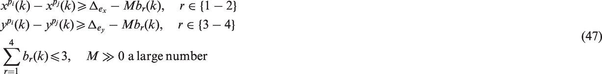
The state-space model used in MPC formulation for the path-planning problem is discussed here. The model for the path-planning stage consists of the following double integrator differential equation describing vehicle dynamics as
Subsequently the linear discrete time-invariant model is
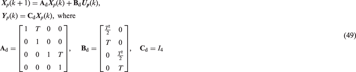
Collision avoidance is ensured by incorporating integer constraints, and minimising the objective function given by
Overprediction and control horizon of length N and M. 
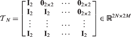
The incremental state matrices are defined as

Once the optimal solution is calculated, the set of waypoints serves as the reference trajectory
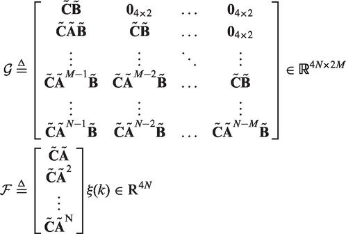
Prediction model
The prediction model following the incremental state-space formulation,
36
can be obtained as

Road constraints
The road constraint for the vehicle position 
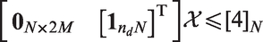
Repeating equation (54) along the prediction horizon N, yields


Note that in this study only straight roads are considered to formulate the road boundary constraints. The model responses are evaluated for vehicle running on a three-lane straight road though the same formulation can be used to model more complex scenarios of curved roads too with appropriate modifications for road geometry, curvature, etc.
Collision avoidance constraints
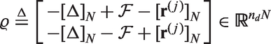
The inequality convex constraints for the distances between the autonomous vehicle and the HDV in matrix form can be written as (recall equation (46)),

The vector 
Replacing the prediction model of equation (53) into equation (58), and rewriting in terms of the optimisation vector 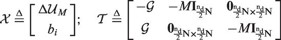
Guaranteeing activation of at least one constraint of (47) by

Path-planning controller
In this work, both path-planner and tracking controllers obtain optimal control vector 
The matrix 
The optimal control vector 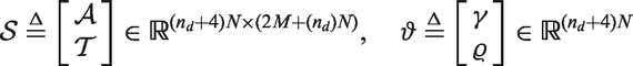
The matrix 
Tracking controller
An adequate mathematical model of the system is an important step in designing a control system. A plant cannot be stabilised if the model description is inadequate.
The tracking controller needs an accurate description of vehicle dynamic characteristics in order to control the vehicle behavior. In the present work, we have used a linear MPC to design the tracking controller. The controller performance is evaluated for two different plant models, namely, the bicycle model and the 12-dof model.
Tracking references
As discussed in previous section, the outputs of both the linear vehicle models are 
In equation (63), K us is the understeering gradient. The value of K us for the vehicle under study is 0.95 °/g.
Cost function
The objective function to be minimised to ensure the vehicle follows desired trajectories is the same as given in equation (50) with the difference that the states here are
Prediction model
The prediction model remains the same as given in equation (53) with appropriate change in dimensions of system state matrices of vehicle models instead of path-planner.
Control constraints
The control constraints are incorporated in the scheme and are written in terms of 

From equations (65) and (64) we obtain

Finally, equation (66) can be written in terms of 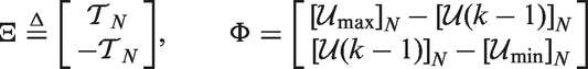

Model predictive controller
Finally, we obtain an optimal control vector 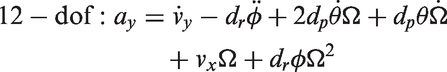
The objective function of equation (68) is minimised using Matlab's built-in function quadprog to obtain the optimisation vector
Parameters of the MPC path-planner.
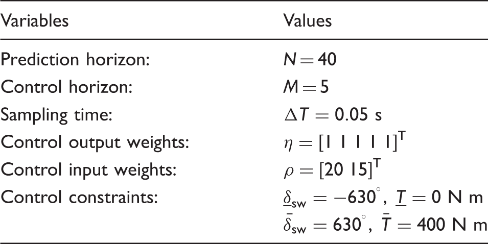
The actuator constraints are set according to the saturation limits. An equal weight is given to all control outputs η in order to track all vehicle dynamics characteristics (
Results
The scenario description for the cooperative obstacle avoidance manoeuvre is shown in Figure 12(a). The vehicles are sharing plans with one another. Vehicle 1 is in the first lane ( (a) Scenario description: double lane change event; (b) steering wheel angle; (c) engine torque.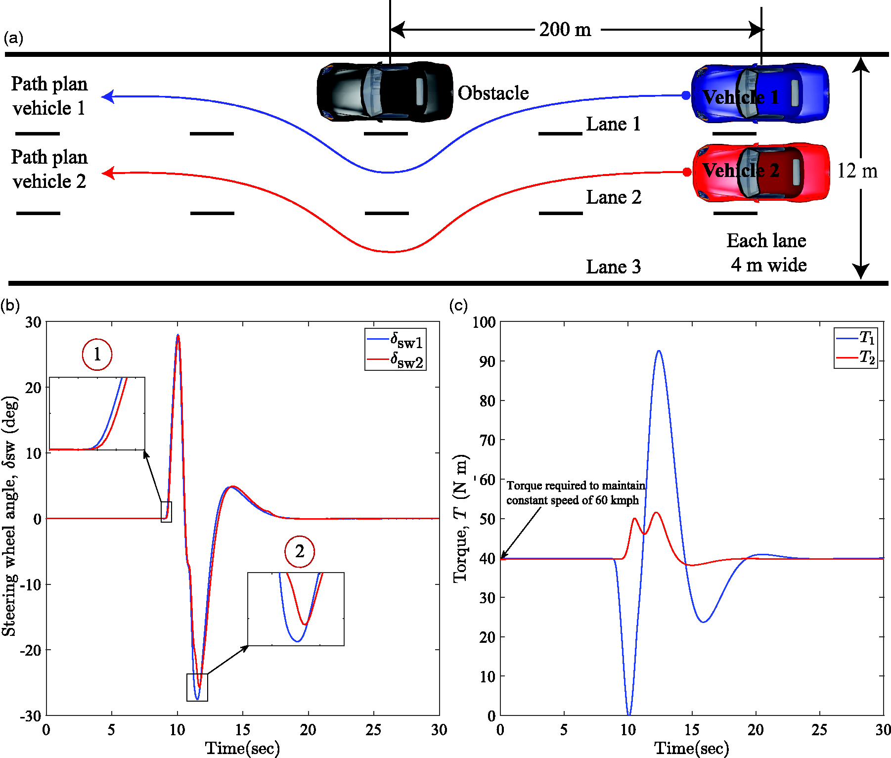
The co-simulation study was performed using the path-planning and tracking controller model and the nonlinear complex vehicle dynamics model built in CarSim. Both the vehicles are able to negotiate the obstacle in a cooperative manner. The results are discussed below.
The control inputs (steering
Initially, both vehicles start their motion with the same torque. This is because the vehicle has to overcome the rolling resistance and aerodynamic drag which is roughly equal to 125 N for the vehicle speed of 60 km/h. This force has to be counteracted by an engine torque of 40 N m in order to maintain a constant speed of 60 km/h. Vehicle 1 brakes more aggressively as it sees the obstacle first as a result the torque decreases. Once it negotiates the obstacle by turning towards the left, the torque increases again to avoid the obstacle quickly. Eventually it comes back in the same lane and the torque again becomes constant, i.e. 40 N-m (torque required to maintain the same reference preset speed of 60 km/h). Vehicle 2 on other hand just swivels out on lane 3 and its torque increases to avoid colliding vehicle 1.
The trace of vehicle trajectory obtained from the animation interface of CarSim cosimulation is shown in Figure 13. The tracking controller responses are shown in Figure 14. The model outputs (shown using solid lines) are compared against the references (shown with broken lines) generated by the path-planner and steady-state yaw rate reference.
Cooperative double lane change event in CarSim. Comparison of model outputs against the reference inputs for the cooperative path planning and tracking controller: (a) Longitudinal versus lateral position; (b) Longitudinal velocity; (c) Lateral velocity; (d) Yaw rate.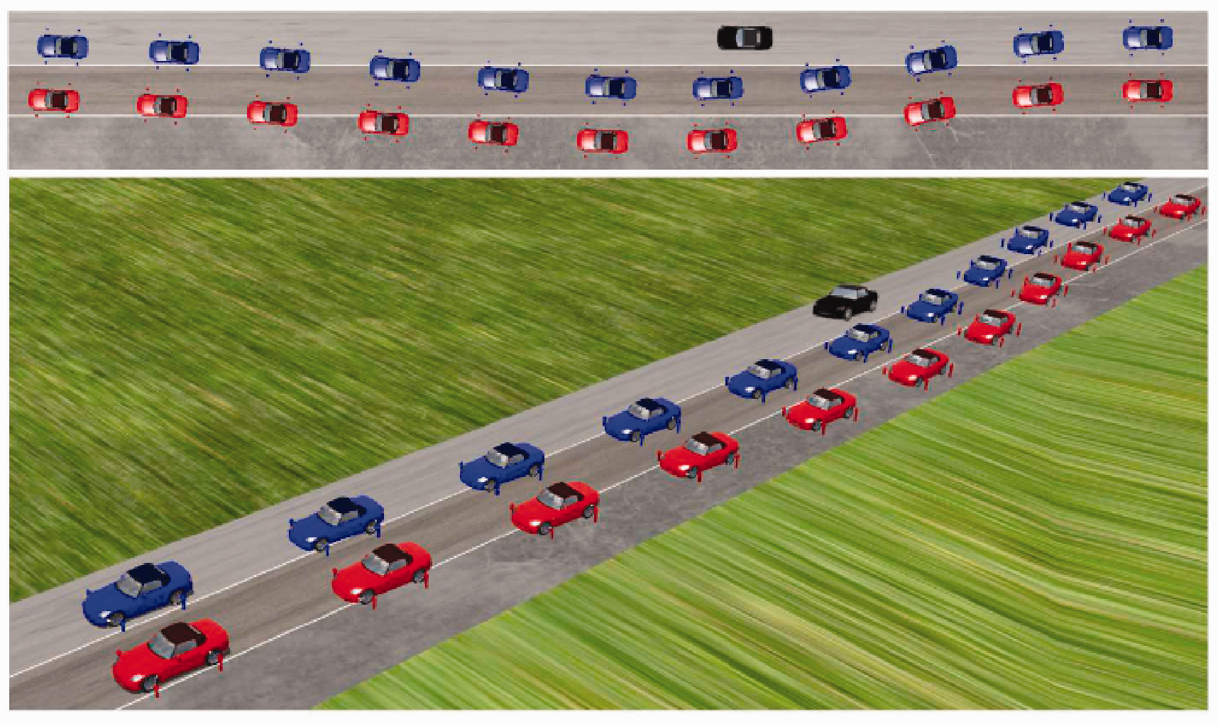
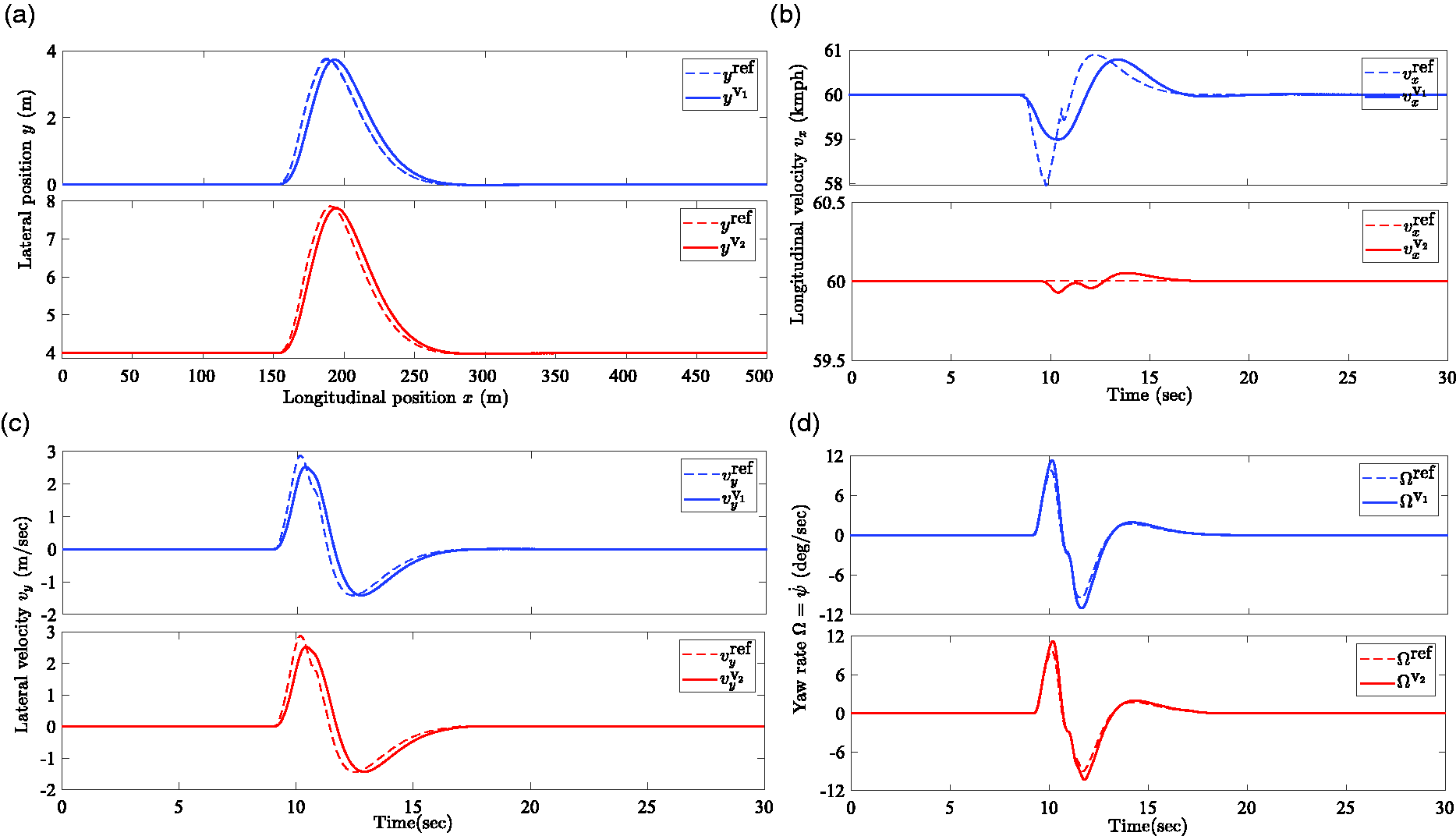
The vehicle path x – y trajectories are shown in Figure 14(a). Vehicle 1 starts in lane 1 and vehicle 2 starts in lane 2. Both the vehicles share each other trajectories (x, y coordinates and longitudinal and lateral velocities v
x
, v
y
). Vehicle 1 can foresee the stationary obstacle in addition to the shared states of vehicle 2. As it encounters the obstacle, it steers to left moves in the second lane and eventually returns back to the same lane. At the same time, vehicle 2 moves in the third lane in order to make way for vehicle 1 and returns back to its lane after the later has negotiated the obstacle. The important thing to note here is that the motion of vehicle 2 is delayed as it takes steering action only when vehicle 1 starts manoeuvring into its lane. Both vehicles are able to track the reference trajectories and a smooth lane change manoeuvre is made. The tracking errors are shown in Figure 15.
Lateral tracking errors of vehicles 1 and 2.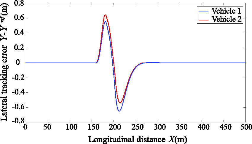
The vehicle longitudinal velocity is shown in Figure 14(b). The velocity of vehicle 1 decreases initially because the torque input decreases as it approaches the obstacle. After it negotiates the obstacle, its velocity increases and returns back to the preset reference value of 60 km/h. The velocity variation for vehicle 2 is not substantial. Both the vehicles are able to track the lateral velocity and yaw rate inputs sufficiently well as shown in Figure 14(c) and (d).
The evolution of other remaining states of the 12-dof model for both vehicle 1 (solid-lines) and vehicle 2 (broken-lines) is shown in Figure 16. The CG displacement z shows a minor variation due to load transfer. As the vehicle encounters the obstacle, it swivels out of the lane towards left. Due to the lateral load transfer, the outer left wheels are compressed and the inner right wheels jack up as seen in wheel jounce responses. As the vehicle rolls out of the turn (anticlockwise direction), the roll angle is positive and a little over 1°. The vehicle pitch also shows a similar trajectory though it value is very small as the vehicle is operating nearly at a constant speed. The rear wheel speeds initially decreases because of reduction in wheel torques as the vehicle approaches obstacle. They regain their initial preset references once the vehicle pasts obstacle.
Evolution of the remaining vehicle states for the cooperative path planning and tracking controller using 12-dof model.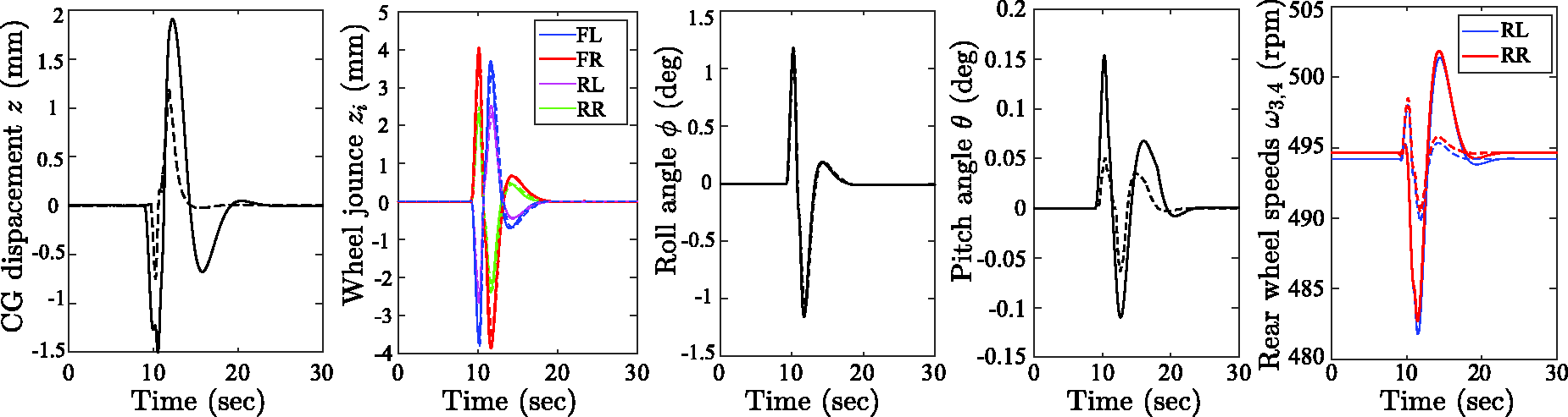
As suggested by an anonymous reviewer, the lateral acceleration and lateral and vertical wheel forces resulting from load transfers are shown in Figure 17. It gives the reader an idea of the magnitude of forces encountered in a normal on-road driving scenario far away from the boundaries of the dynamic envelope.
Lateral acceleration, lateral and vertical tyre forces for vehicle 1 undergoing the obstacle avoidance manoeuvre.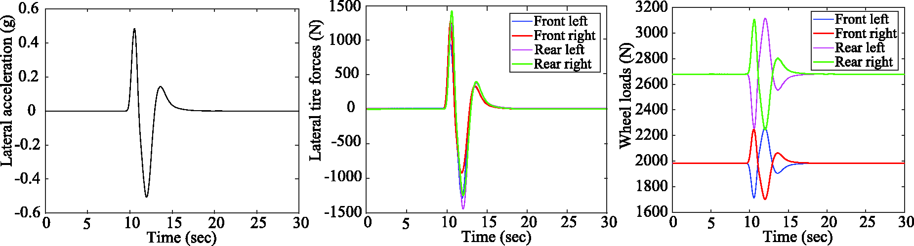
Model evaluations
In this section we investigate the performance of our model at different speeds and compare the responses obtained from our model against the bicycle model predictions.
Performance evaluation at different speeds
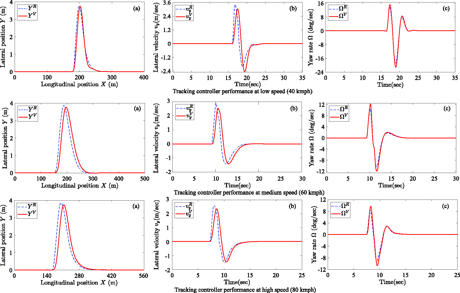
To evaluate the performance of the 12-dof model for a range of operating speeds we have compared the tracking controller results at 40, 60 and 80 km/h in Figure 18(a), (b) and (c), respectively. For this we used different initial conditions of vehicle velocity v
x
for linearing the 12-dof model as Vehicle longitudinal and lateral positions X – Y. The vehicle is able to track reference path trajectory sufficiently well in all three cases. A sufficiently smooth double lane change manoeuvre is performed. The tracking is better at low speed and inferior at high speeds but still the match is pretty good. This is obvious because of lag in following the reference path at high speeds because of the second-order actuator dynamics. Lateral velocity v
y
. The vehicle is able to track the lateral velocity quite well in all the three cases. The lateral velocity decreases as speed increases. Yaw rate Ω. The vehicle roughly maps the yaw rate input. The reason for the in all three cases mismatch is because a steady-state yaw rate measure is used as a tracking reference which is slightly less than dynamic yaw rate. Tracking controller responses at different speeds: (a) Longitudinal versus lateral position; (b) Lateral velocity; (c) Yaw rate.
Comparison against the bicycle model
The vehicle dynamic responses ( Comparison of model responses of 12 dof model and bicycle model: (a) Steering wheel angle; (b) Lateral versus longitudinal position; (c) Lateral velocity; (d) Yaw rate.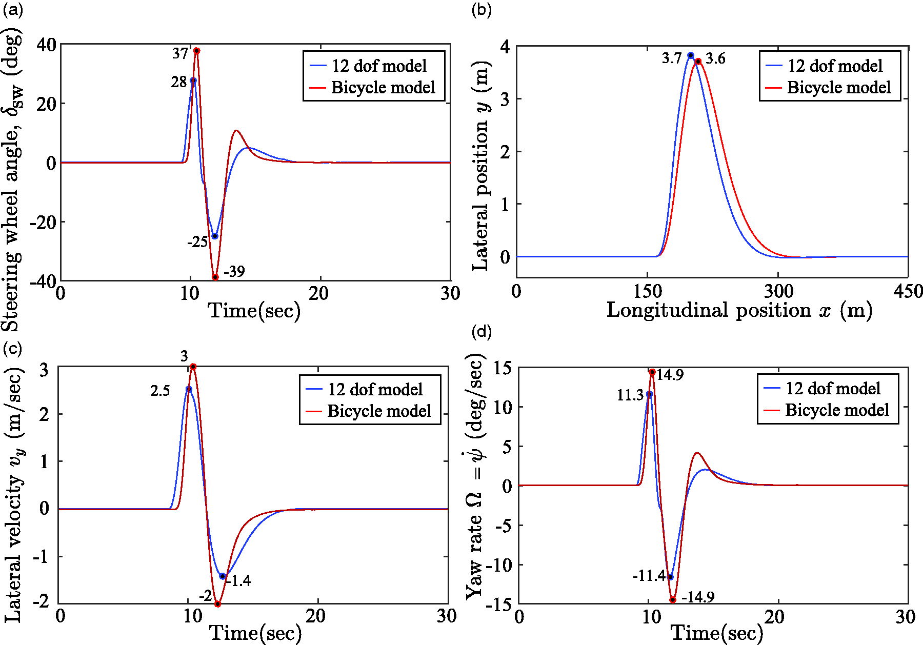
The steering angle input computed by the tracking controller using bicycle model is on the higher side as compared with the 12-dof model (see Figure 19(a)). We have earlier seen in Model comparisons section that for the same steering angle input the dynamic behaviour of the vehicle obtained from the 12-dof model matches closely with the sophisticated CarSim model. This implies that if higher values of steering wheel angle are used in a real vehicle according to bicycle model predictions it will result in high values of other dynamic characteristics, which will eventually result in inaccurate tracking of the reference trajectories.
Regarding path tracking, the bicycle model underpredicts the lateral position as compared to the high fidelity model as shown in Figure 19(b) even though it uses a high value of vehicle steering input. This justifies the need of a model of increased complexity for tracking the vehicle trajectory.
There is a substantial amount of difference in the lateral velocity v
y
and yaw rate Ω responses between the two models (see Figure 19(c) and (d)). The reason for this mismatch is the unmodelled lateral dynamics of the bicycle model as opposed to the 12-dof model. For instance, refer to equation (5) and
Bicycle model, 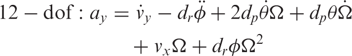
The effect of pitch θ and roll φ angle is evident on the value of lateral acceleration a y , which is missing in the bicycle model but captured in the 12-dof model. This shows the superiority of the 12-dof model in tracking the reference trajectories generated by the path-planning MPC.
Conclusion and future work
This work gives a useful insight by evaluating the controller performance for different models. The high fidelity nonlinear vehicle model of intermediate complexity inclusive of roll, pitch and suspension jounce motions is developed. In addition to this, two simplified models namely the kinematic model and the bicycle model were also developed. The models have been compared for a single lane change manoeuvre and it has been established that the 12-dof model emulates the real vehicle dynamic characteristics fairly well. This nonlinear model is subsequently linearised to take an account of different operating conditions.
In the next part, the paper addressed the problem of path-planning and tracking controller for an autonomous vehicle considering the trajectories of other autonomous vehicle. The problem is solved using a hierarchical MPC design with MIQP at the planning layer. Integer constraints are incorporated to ensure collision avoidance between the autonomous vehicles and stationary obstacle. Control actuation constraints have also been incorporated in the proposed approach. To evaluate the effectiveness of the method, numerical simulations are performed for a cooperative double lane change manoeuvre, which demonstrate the effectiveness of the proposed method. The tracking controller is able to follow the references and the method is quite appropriate to attain the on-road autonomous driving environment. This is because the linear tracking controller uses only 22 state variables to control the high fidelity nonlinear vehicle model in CarSim.
In future, the current method with linear MPC will be compared with nonlinear MPC and other alternatives will be evaluated to account for probabilistic trajectories and soft constraints. An initial investigation of these concepts has been evaluated by the Viana et al. 42 Moreover the goal is to demonstrate cooperative autonomy in an urban environment where the obstacles are moving human-driven vehicles as opposed to stationary obstacles. This work will be extended to incorporate moving obstacles with probabilistic trajectories coming from the human driver model. 43
Finally, this algorithm is planned to be implemented in a real-time vehicle operation and that can be taken up as the future developmental work.
Footnotes
Acknowledgements
This project comprises a consortium with six partners, namely, Applus IDIADA, Cosworth Electronics, Connected Places Catapult, Westfield Sportscars, SBD Automotive and Cranfield University. This work is planned to be implemented in real vehicles by the end of the project.
Declaration of Conflicting Interests
The author(s) declared no potential conflicts of interest with respect to the research, authorship, and/or publication of this article.
Funding
The author(s) disclosed receipt of the following financial support for the research, authorship, and/or publication of this article: This work has been supported by Innovate UK within the scope of the project grant MuCCA ‘Multi-Car Collision Avoidance’.