
Abstract
This study presents a novel application of the Transmission Line Matrix Method (TLM) for the modelling of the dynamic behaviour of non-linear hybrid systems for computer numerical control (CNC) machine tool drives. The application of the TLM technique implies the dividing of the ball-screw shaft into a number of identical elements in order to achieve the synchronisation of events in the simulation, and to provide an acceptable resolution according to the maximum frequency of interest. This entails the use of a high performance computing system with due consideration to the small time steps being applied in the simulation. Generally, the analysis of torsion and axial dynamic effects on a shaft implies the development of independent simulated models. This study presents a new procedure for the modelling of a ball-screw shaft by the synchronisation of the axial and torsion dynamics into the same model. The model parameters were obtained with equipments such as laser interferometer, ball bar, electronic levels, signal acquisition systems, etc. The MTLM models for single and two-axis configurations have been simulated and matches well with the measured responses of machines. The new modelling approach designated the Modified Transmission Line Method (MTLM) extends the TLM approach retaining all its inherent qualities but gives improved convergence and processing speeds. Further work since, not the subject of this paper, have identified its potential for real-time application.
Background
Ford 1 proposed that the design process of any high precision computer numerical control (CNC) machine tool must embrace error avoidance, error measurement, and error compensation techniques in order to achieve an ever increasing demand for greater accuracy and therefore a more stringent performance specification. The measurement of the repeatable time and spatial errors can allow compensation methods to be applied to the machine for correction of those errors provided sufficient resolution has been allowed for in the design, with the absolute limit on accuracy for a particular machine being defined by its measured repeatability figures and the responsiveness of its compensating axes. The main areas of concern affecting component accuracy are environmental effects, user effects and the machine tool static and dynamic accuracy. The sources of error confined to a machine tool are geometrical inaccuracies, thermally induced errors and load errors.
Machine tool feed drive modelling and system identification
Pislaru et al. 2 stated that the modelling used for designing high performance CNC machine tool feed drives should accurately represent the system consisting of three cascaded closed loops for acceleration, velocity and position control. They utilised a modular approach and a hybrid modelling technique which included for distributed load, explicit damping coefficients, backlash and friction. The model was a combination of distributed and lumped elements described by partial differential equations and ordinary differential equations as proposed by Bartlett and Whalley. 3
Holroyd et al. 4 modelled the dynamic behaviour of a ball-screw with moving nut using a finite element approach. The ball-screw was divided into a large number of elements and contact/boundary conditions for each element and adjacent ones were studied. An important conclusion was that the natural frequencies of the ball-screw system vary in time due to two causes: (a) the lateral restraint produced by the nut when the screw was transversally vibrated and (b) the relation between screw torsion, axial motion and worktable/saddle tilt.
Transmission line matrix method
The transmission line matrix (TLM) method belongs to the general class of differential time domain numerical modelling methods. It is used to solve time-dependent or transient problems, thus involving ordinary and partial differential equations (PDE).
The application of TLM to the modelling of fluid systems by Boucher and Kitsios 5 and mechanical systems by Partridge et al. 6 implies the same representation used in the hybrid approach by Pislaru, 2 i.e. lumped parameter modules, components with localised dynamic effects and distributed parameter modules. The difference resides on the fact that transmission line equations introduce natural time delays between components due to the wave propagation speed in a transmission line. Therefore, distributed components must be divided into a number of identical elements in order to achieve the synchronisation of events in the simulation, and to produce acceptable resolution according to the maximum frequency of the simulation. This characteristic gives the possibility to include the effect of the nut movement suggested in Holroyd’s et al. 4 approach.
Johns and Beurle 7 described the two equivalent circuits used in the TLM technique: the stub and the link circuits. TLM links are two-port one-dimensional building blocks that can be used for one-, two- or three-dimensional modelling. TLM stubs are one-port units which can be used for solving circuits and equations, and are used in multi-dimensional modelling to complement TLM links. Links are used for modelling distributed parameter elements and stubs for lumped parameter elements.
Christopoulis 8 stated that any electrical circuit could be represented as a network of transmission line circuits by simply replacing the reactive elements with corresponding stubs. Variables such as voltage and current are regarded as discrete pulses bouncing at a velocity to and from nodes of these stubs at each time step. The voltage and current in each element are determined from the incident and reflected pulses in each stub. He demonstrated the transmission line and its Thevenin equivalent.
The MTLM stub, taking into account changes of sample time was applied to the modelling of a rotor shaft arrangement by Partridge et al., 6 where Castaneda 9 demonstrated improved robustness and accuracy of the simulation. A reduction of 40% in the number of mathematical operations and almost 35% reduction in the mean square modelling error figures were achieved. This method of approach was utilised for this application.
Single axis CNC test rig
The single-axis test rig (Figure 1a) represents the y-axis of a vertical machining centre (VMC). The single axis is fitted with a Heidenhain TNC-426PB motion controller, a SIMODRIVE-611 Siemens inverter, and a ball-screw arrangement directly coupled to a permanent magnet synchronous motor.
(a) Test rig and (b) test rig block model.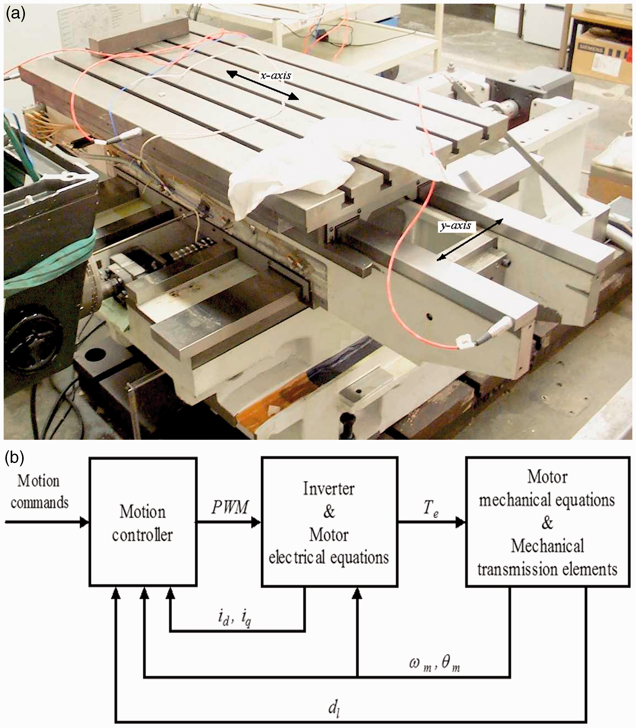
The Heidenhain 10 TNC-426PB motion controller offers digital control of functions such as interpolation, position control, speed control, current control and provides PWM signals to the inverter unit. The control of each axis is implemented with an algorithm following the principle of cascade control in conjunction with velocity and acceleration feed forward.
The SIMODRIVE-611 consists of a common feed module that provides the DC voltage link from the power supply mains and a set of drive modules that activate each motor. In the case of the test rig, the drive module consists of a power module (inverter) and an interface card that communicates with the TNC-426PB motion controller.
The nut of the ball screw system is preloaded and the screw shaft is mounted on preloaded bearings in a fixed–fixed configuration.
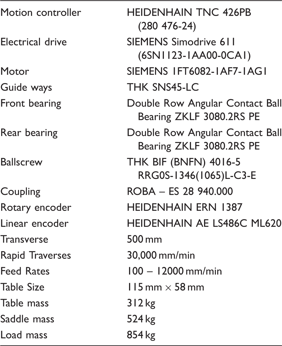
Test rig specification.
TLM method applied to CNC machine tool feed drive
Motion controller
Heidenhain
10
operates with position and velocity control in cascade with feed forward capability as shown in Figures 2 and 3. Seborg et al.
11
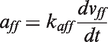
concluded that feed forward control improves trajectory tracking compensating for the effect of disturbances before they affect the response of the controlled system. The velocity feed forward path connects the reference position to the velocity loop through the gain, kff (Figure 3). When the position profile changes, the velocity feed forward transfers immediately that change to the velocity command. This speeds up the system response, thus not relying solely on the position loop. The primary shortcoming of velocity feed forward is that it induces overshoot when changes on the velocity direction occur. Acceleration feed forward eliminates the overshoot caused by velocity feed forward without reducing loop gains. The basic principle of feed forward control is to inject the position and velocity set points and their correspondent first derivatives at appropriate points in the control loops. Heinemann and Papiernik
12
demonstrated that the following errors are minimised, thus achieving a significant increase in the dynamic response to position and velocity set point changes.
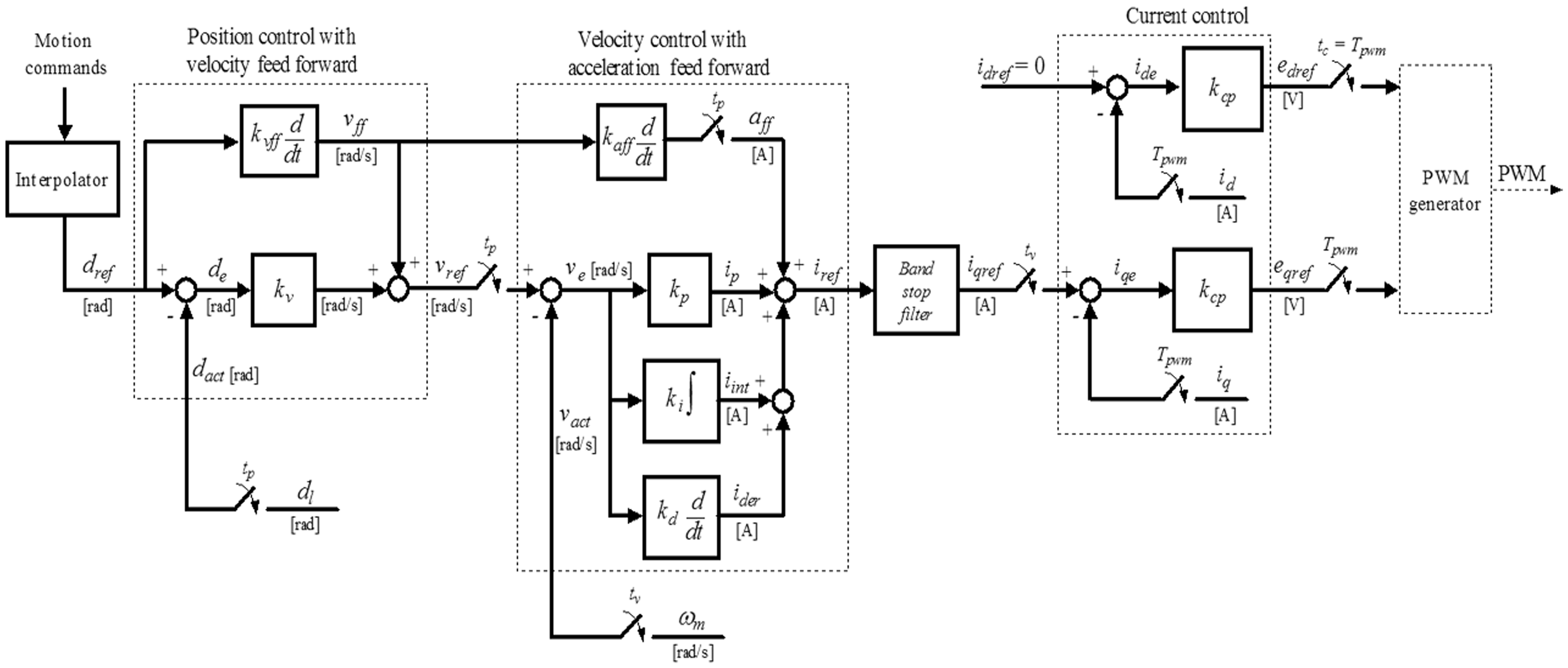
Motion controller block model. Motion controller flow model.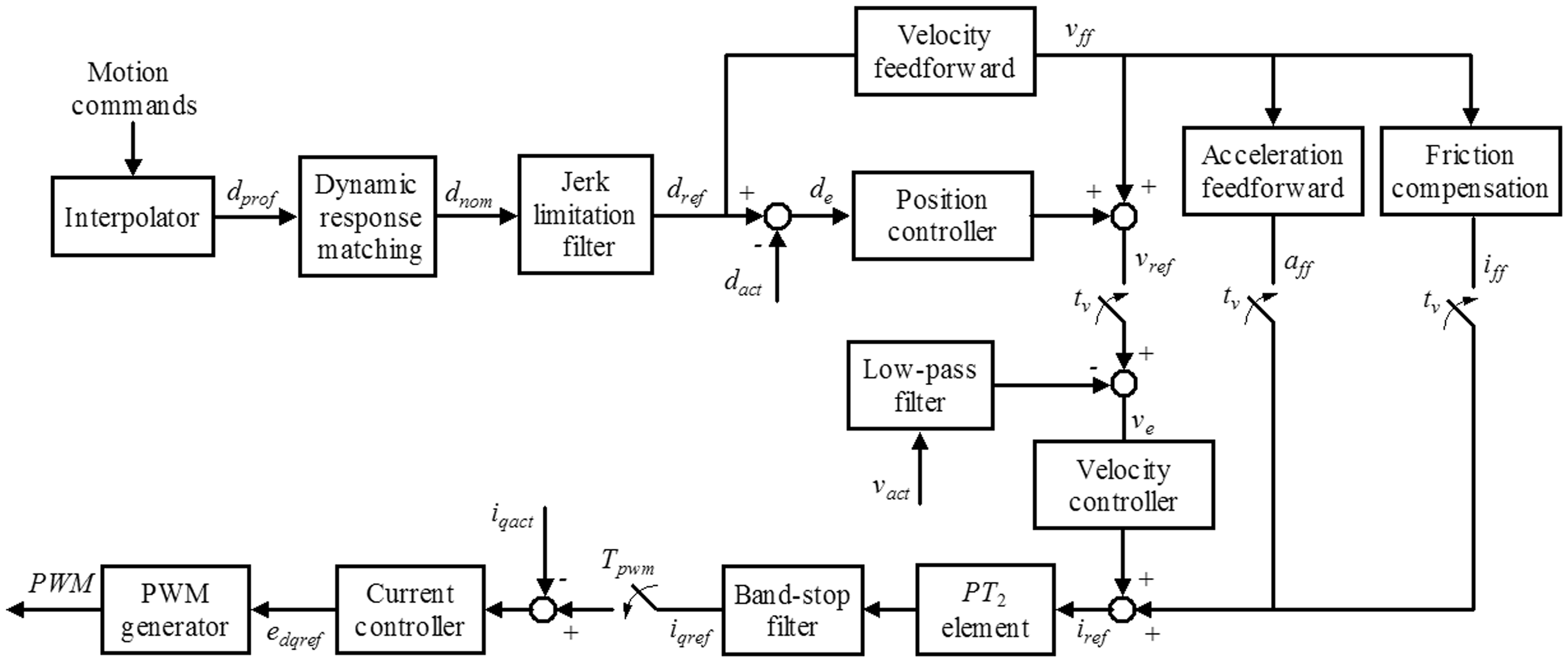
Altinas 13 demonstrated that the interpolator (Figure 2) calculates a velocity profile v (t), according to defined motion commands: feed rate (fr), maximum acceleration (amax), maximum jerk (jmax), and desired displacement (d). The velocity profile is then used to generate the set of reference positions in order to achieve a smooth velocity transition.
Koren 14 and Bullock 15 demonstrated that linear and circular interpolation, respectively, are performed to keep the tool path velocity constant at the given feed rate along a straight line in a plane of motion.
If the system has multiple axes, the motions of individual axes are co-ordinated. When the individual axes are not co-ordinated, each of the axes will start moving at the same time, but finish at separate times producing slew motion as defined by Hugh. 16
The interpolator overcomes this effect using an interpolation technique. Position values from the interpolator can be filtered in order to obtain a smoother motion profile. The filtered values constitute the reference position signals for the position controllers.
The Heidenhain TNC426PB
17
motion controller (Figure 3) was implemented in software featuring the algorithms for position, velocity and current control at different sampling rates.
10
That is:
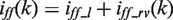
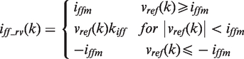
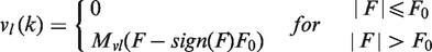
The interpolator generates a reference position value de every 3 ms. The position controller generates a reference velocity value vref every 3 ms. The velocity controller generates a reference current value iqref every 0.6 ms. The current controller gives a reference voltage value edqref to the PWM generator at a rate of 0.2 ms. The dynamic response-matching filter (first order delay filter) was used to delay the position profile signal according to the transient response during acceleration and deceleration (the equivalent position time constant of the closed position control loop). Delay values can be set in the interval of 1–255 ms. The jerk limitation filter was used to adapt the position profile to the machine dynamics in order to attain high machining velocity. The coefficients of the filter were calculated according to the minimum order of the filter and the tolerance for contour transitions. The PT2, second order element was used to include a delay in the reference current (iref) to damp the frequency interference oscillations (circa: 0.3–2 ms). Sliding friction was compensated within the range of the velocity controller by compensating the sliding friction at low velocity and at the rated velocity of the motor. The compensation at low velocity was achieved by feeding forward the reference current value (measured at approximately 10 rpm) at every change in direction. The compensation at the rated velocity was achieved by feeding forward the current iff_rv according to the value of the reference velocity (equation (2)). A delay filter was included to prevent overcompensation when the traverse direction was reversed at high feed rates.
iffm is the reference current measured at the rated velocity of the motor; iff_l is the reference current at 10 rpm and kiff is the scaling factor.
Position controller with velocity feed forward
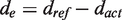
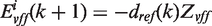
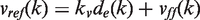
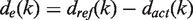
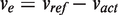
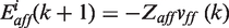
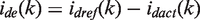
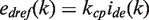
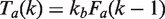
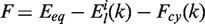
The position controller evaluates the difference between the reference and actual position value dact (from the rotary or linear encoder) to calculate the position error de. A reference velocity value (vref) is then generated every ts seconds according to the following
kb is the force to torque constant of the ball screw.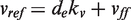
The TLM model for this module is represented by equations (3) to (7) for a sample time ts = 3 ms.
By a combination of Christopoulis
8
and Castaneda
9
theory
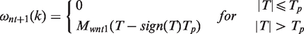
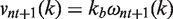
Velocity controller with acceleration feed forward
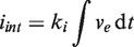
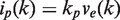
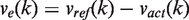
The velocity controller evaluates the difference between the reference and actual velocity value (vact) measured with a rotary encoder attached to the motor. A reference current value (iref) is generated every ts s by a Proportional-Integral-Differential (PID) strategy.
Acceleration feed-forward is used in parallel with the velocity controller in order to minimise the spikes caused by changes in velocity direction. A signal iht (holding current) is added to the acceleration feed forward to counterbalance the axis load when the axis in the vertical position.
Equations (13) to (18) represent the TLM model for this module (ts= 0.6 ms). The following relationship calculates the reference current signal


Band-stop filter
Heidenhain 17 states that a filter is generally used in the velocity feedback to damp the fundamental frequency of the control system, when it is higher than 500 Hz. A first-order low-pass filter is used when the oscillation frequency is between 500 and 700 Hz. A second-order low-pass filter is used if the oscillation frequency is higher than 700 Hz.
When the controlled system is insufficiently damped, it will be impossible to attain a sufficiently short settling time without inducing oscillations in the step response of the velocity controller. The step response will oscillate even with a low proportional factor. A second-order lag element (PT2) is used to include a delay in the reference current (iref) to damp the frequency interference oscillations.
A band-rejection filter is included in series with the PT2 element to damp oscillations that cannot be compensated by the differential factor of the velocity controller, the PT2 element or the low-pass filter.
Mathworks
18
state these digital filters are generally modelled as implementations of the standard difference equation
b and a represent the numerator and denominator coefficients of the filter and N is the order of the filter.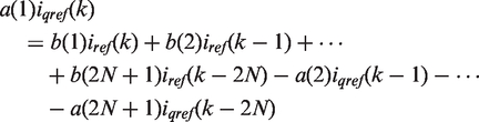
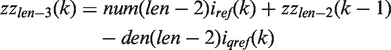
The band-stop filter was implemented as indicated by Mathworks
19
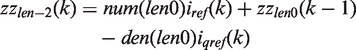
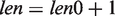
in the transposed direct-form II structure of equation (27). This is a canonical form that has the minimum number of delay elements. At sample k, the routine computes the difference equations as follows


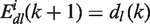
Current controller
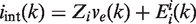
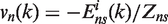
The current controller is an implementation of the model when the integral term kci is equal to zero.
Castaneda
9
developed the model shown and converted to the TLM transform of equations which are presented as

Inverter and motor (electrical)
Moreton
20
describes the voltage relationships and provided the general equation for a permanent magnet synchronous motor (PMSM). Simon
21
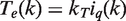
explained the Clarke /Park transformation and their inverse relating the vector currents used for the generation of electromagnetic torque (Figure 4a).
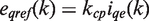
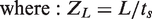
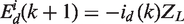
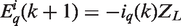
TLM model for the motor and coupling. (a) Motor electrical equations, (b) TLM model of the motor and coupling, (c) reduced TLM model and (d) Thevenin equivalent circuit.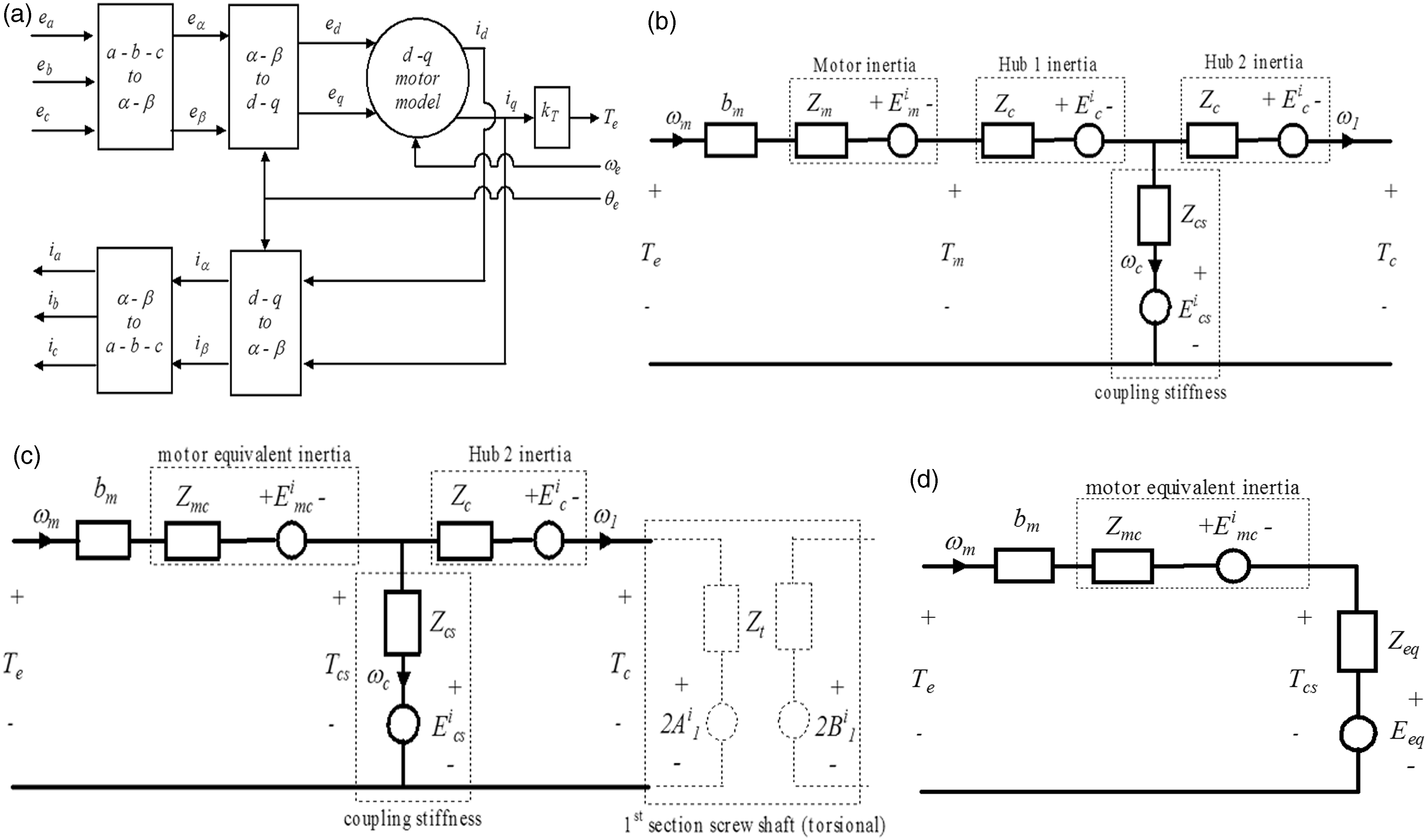
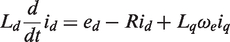
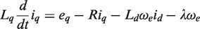
The equations of performance for a PMSM in the d–q coordinate system representation are


Motor mechanical equations and coupling
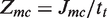
The inertias of the rotary encoder and the coupling (hub 1) can be added to the inertia of the motor to simplify the calculations. Hence
Jmc = motor plus coupling inertia; Jm = motor inertia and Jre = rotary encoder inertia.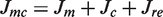
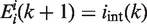
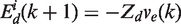
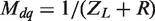
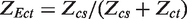
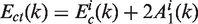
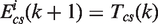
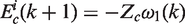
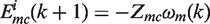
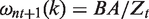
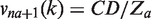
This reduction of the model is possible because those inertias are modelled as lumped parameter elements. The resultant TLM model is illustrated in Figure 4(c) (reduced from Figure 4b).This electric circuit is solved finding the Thevenin equivalent
8
with respect to Tcs (Figure 4d), thus


Screw shaft torsional model
From the theory outlined by Partridge et al., 6 Holroyd et al., 4 and Castaneda, 9 the following model was derived.
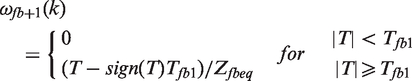
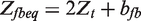
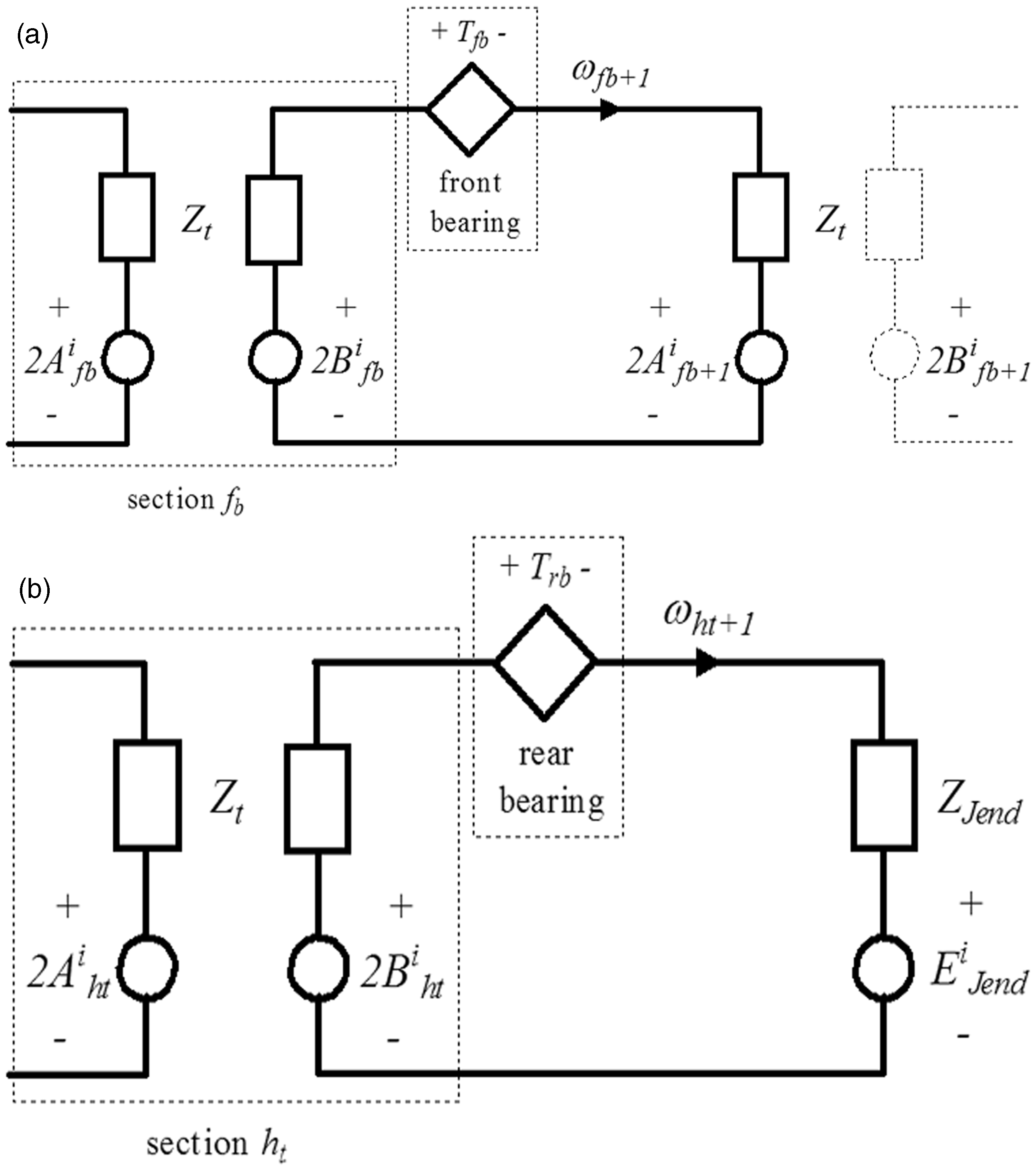
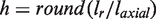
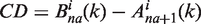
The presence of the supporting bearings in the TLM model of the shaft generates the reflection of pulses arriving to the sections where they are placed. In that case, the propagation of pulses in the TLM model takes place on two specific zones (loops) as it is graphically represented in Figure 5(a). The front bearing is placed on section fb, the nut is on section nt and the rear bearing is on section ht, where
Pulses propagation model for the screw shaft torsional model with moving nut. (a) Without nut and (b) Zone 2 including the nut.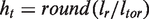


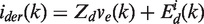
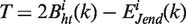
The velocity of the front bearing (ωfb+1) is calculated including the TLM model derived for the bearing's friction
22
(see Figure 6(a)), thus
(a) Section fb of the torsional model. (b) Section ht of the torsional model.


The pulse propagation is defined by


Screw shaft axial model
From the theory outlined by Partridge et al. 6 and Holroyd et al., 4 Castaneda 9 derived the following model.
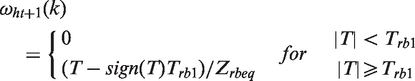
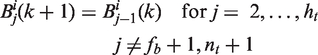
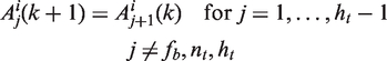
The presence of the supporting bearings and the nut generates the reflection of pulses arriving to the sections where they are placed. This leads to the propagation of pulses on one zone (loops) in the axial model as it is graphically represented in Figure 7.
Pulses propagation model for the screw shaft axial model with moving nut. (a) Without nut and (b) including the nut.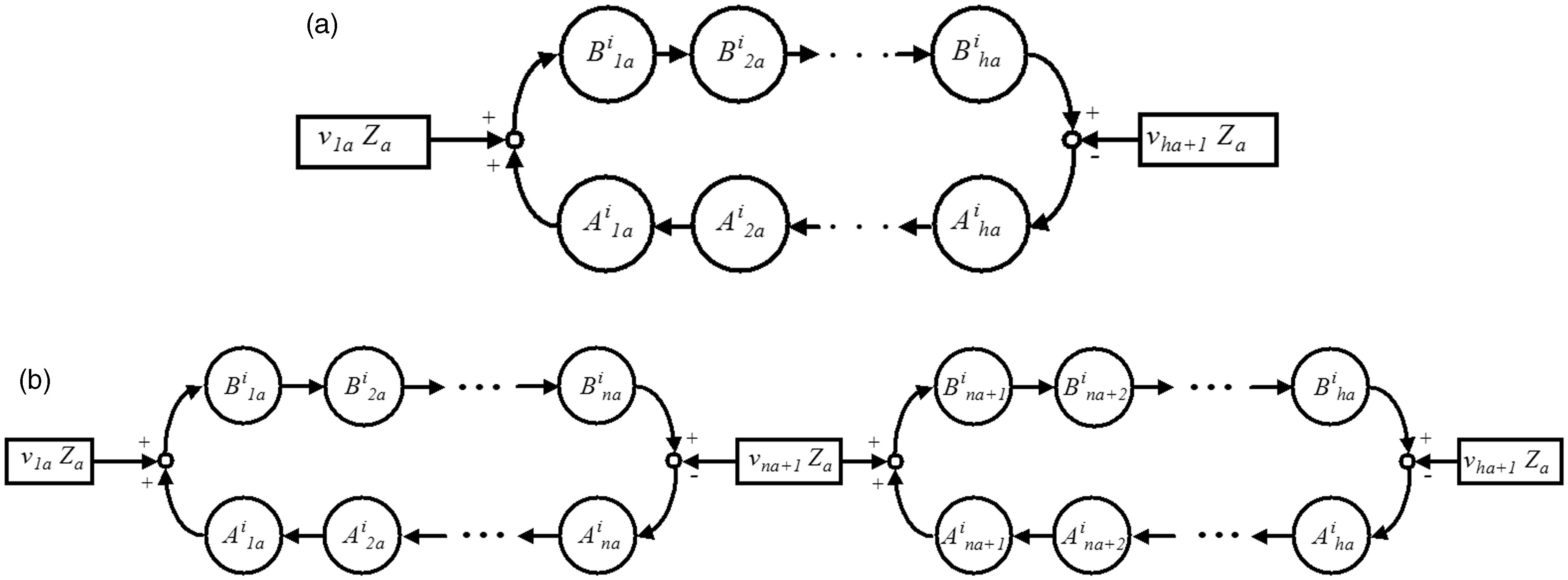
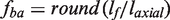
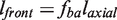
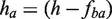
The inclusion of the nut in the model will cause the reflection of pulses arriving to section na, and therefore splits the model in two loops as shown in Figure 7(b). The front bearing is placed on the first section, the nut is on section na and the rear bearing is on section ha, where


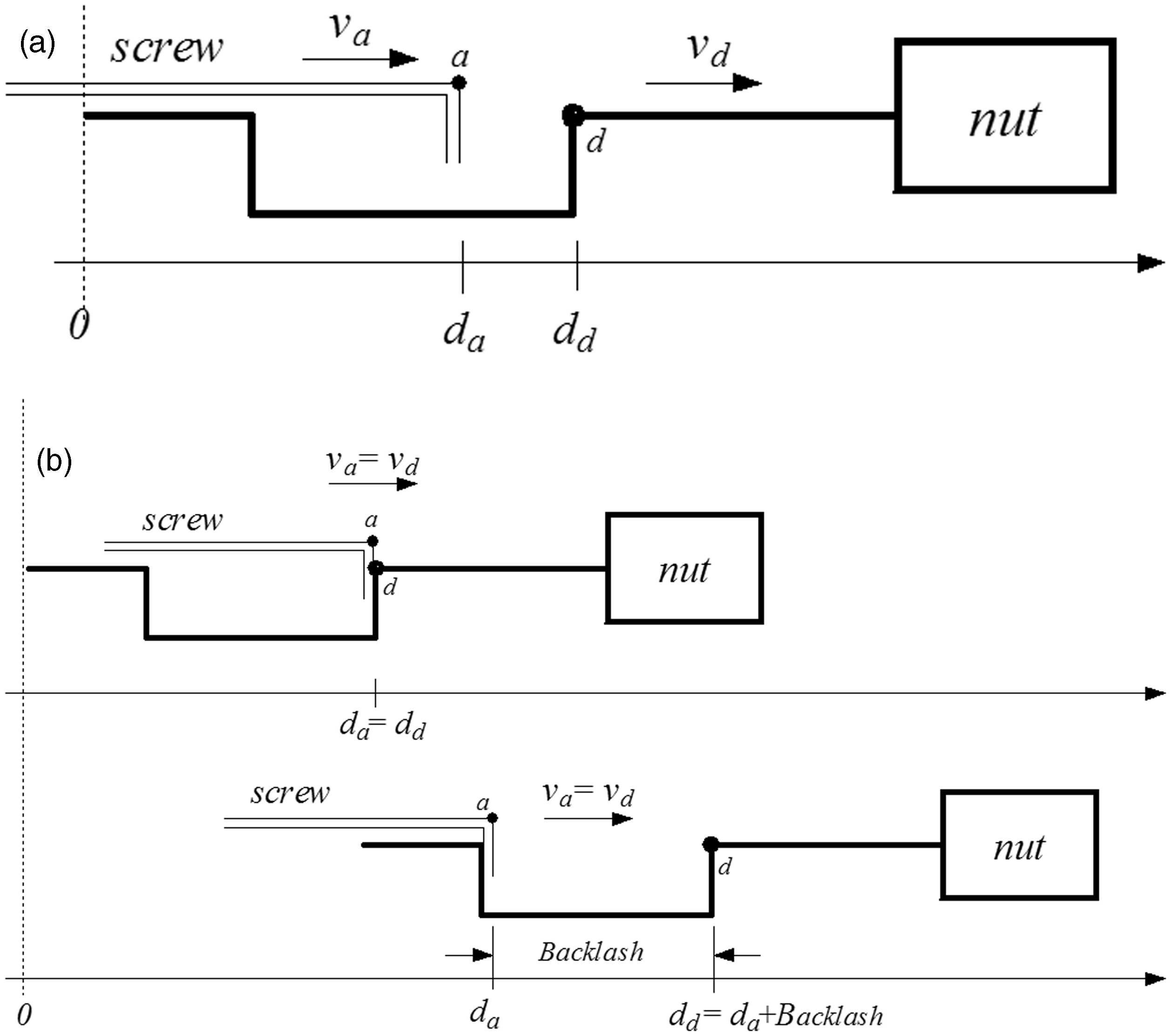
Screw shaft, nut and table
Figure 8 illustrates the connection of the axial and torsional TLM screw shaft models with the nut and table models, thus


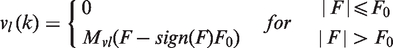
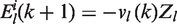
The backlash model presented has been reduced to the following two possible states:
when the screw shaft is not in contact with the nut (Figure 9a) and when the screw shaft is in contact with the nut (Figure 9b). Non-contact if:
– dd ≠ da –dd = da and the direction of motion is negative (nut moving towards the motor). –dd = da + Backlash and the direction of motion is positive. Contact if:
–dd = da and the direction of motion is positive. –dd = da + Backlash and the direction of motion is negative. Backlash model. (a) Non-contact and (b) in contact. TLM model of the connection between nut and screw shaft. (a) Torsional model connextion, (b) axial load connextion and (c) Equivalent model for the connection between nut and screw shaft.
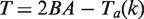
The state in which the axis will start at the beginning of the simulation depends on the following conditions:
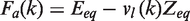
Variables Ta and Fa are zero if the screw shaft is not in contact with the nut. Thus the values for the velocities are given by the following equations


Implementation of two-axis TLM models to a CNC machine tool
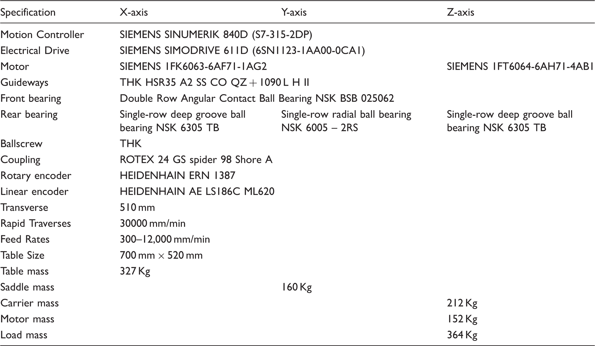
Figure 10(c) shows the three-axis vertical machining centre where the unidirectional Z-axis maximum tool travel is 560 mm, and the bidirectional machining tables X-axis maximum travel and Y-axis maximum travel are both 510 mm. The Siemens 840D CNC controls all the machine tool functions. The spindle speed can be controlled from 60 RPM (revolutions per minute) to 8000 RPM and the maximum axis feed-rates are 12 m/min (fast traverse 30 m/min). The machine utilises Siemens 611 electrical feed drives with permanent magnet synchronous motors (Types 1FK6063 on X- and Y-axis and Type 1FT6064 on Z-axis). The motors for each axis are flexibly coupled to a ball-screw supported by bearings at both ends and utilise linear bearing guide-ways. The Siemens spindle drive unit provides four quadrant operations through a separately excited Siemens DC motor providing a constant torque range 60 RPM to 1500 RPM and above 1500 RPM constant power range (9 KW) to the maximum speed of 8000 RPM.
Machine tool. (a) x–y axis feed drive, (b) block diagram and (c) machine tool and coordinate system.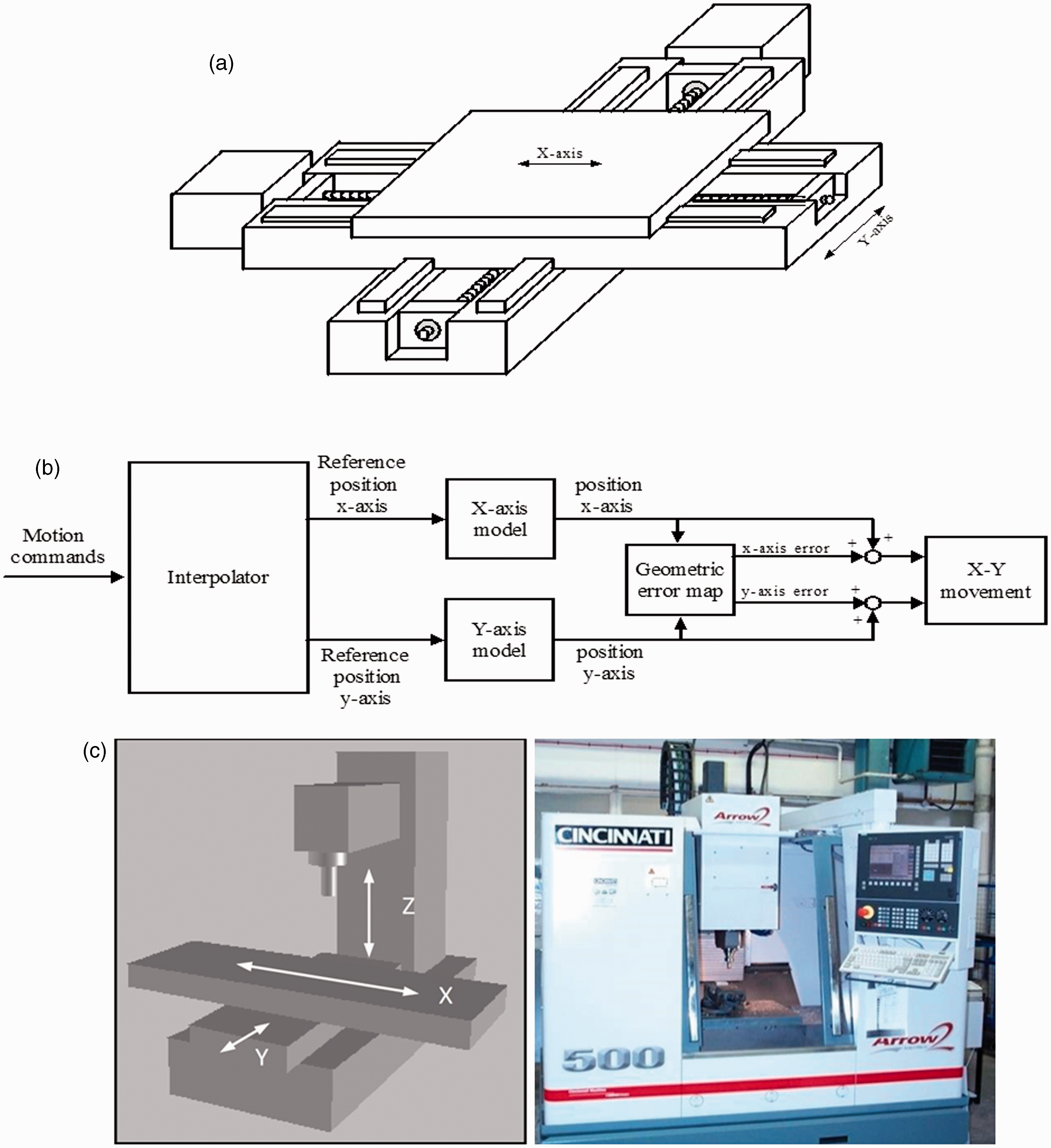
The VMC-500 is fitted with a Siemens SINUMERIK 840D motion controller, which commands the CNC kernel functions for interpolation and position control. The motion controller is connected to the drives and I/O units via a PROFIBUS-DP interface as shown by Siemens. 23 Each axis integrates a SIMODRIVE-611 Siemens inverter and a ball-screw arrangement directly coupled to a permanent magnet synchronous motor. The ball-screw systems incorporate a preloaded nut and the screw shaft mounted on a fixed-supported bearing configuration.
VMC-500 machine specifications.
The main differences between the TNC 426PB and the SINUMERIK 840 D
24
in terms of modelling its behaviour are as follows:
The SINUMERIK 840D includes a velocity response matching filter (first-order delay-filter) used to delay the velocity feed forward signal according to the equivalent position time constant of the closed velocity control loop. The SINUMERIK 840D configuration for this machining centre does not include acceleration (torque) feed forward. A velocity filter is included to damp the resonant frequencies in the closed position loop. A velocity limitation in the form of saturation is included in the position loop. Torque and current limitations in the form of saturation are included in the velocity loop. The velocity controller does not include differential term (PI control). Two additional filters are included in the velocity loop in order to get a filtering process with better time/frequency response. For example, Filter 1 can be configured as the PT2 filter in the TNC 426 PB and filters 2–4 can be combined to get a band-rejection filter with better damping and frequency properties than the band-rejection filter in the TNC 426 PB. The current controllers include integral term (see Motion controller section). The sample time for the interpolator and position controller is 4 ms (cf. 3 ms). The sample time for the velocity controller is 0.125 ms (cf. 0.6 ms). The sample time for the current controller is 0.125 ms (cf. 0.2 ms).
Although the control algorithm is distributed in two different units (SINUMERIK 840D and the plug-in control units), the dynamics acting on the x- and y-axes are modelled as in the single-axis test rig case. The model for the rear bearing mounting has been updated to reproduce the fixed-supported bearing configuration.
The two-axis system is configured as shown in Figure 10(a). Linear and circular interpolation methods described in the Motion controller section are included in the interpolator to coordinate the movement of the axes.
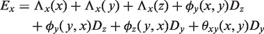
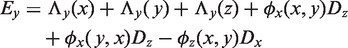
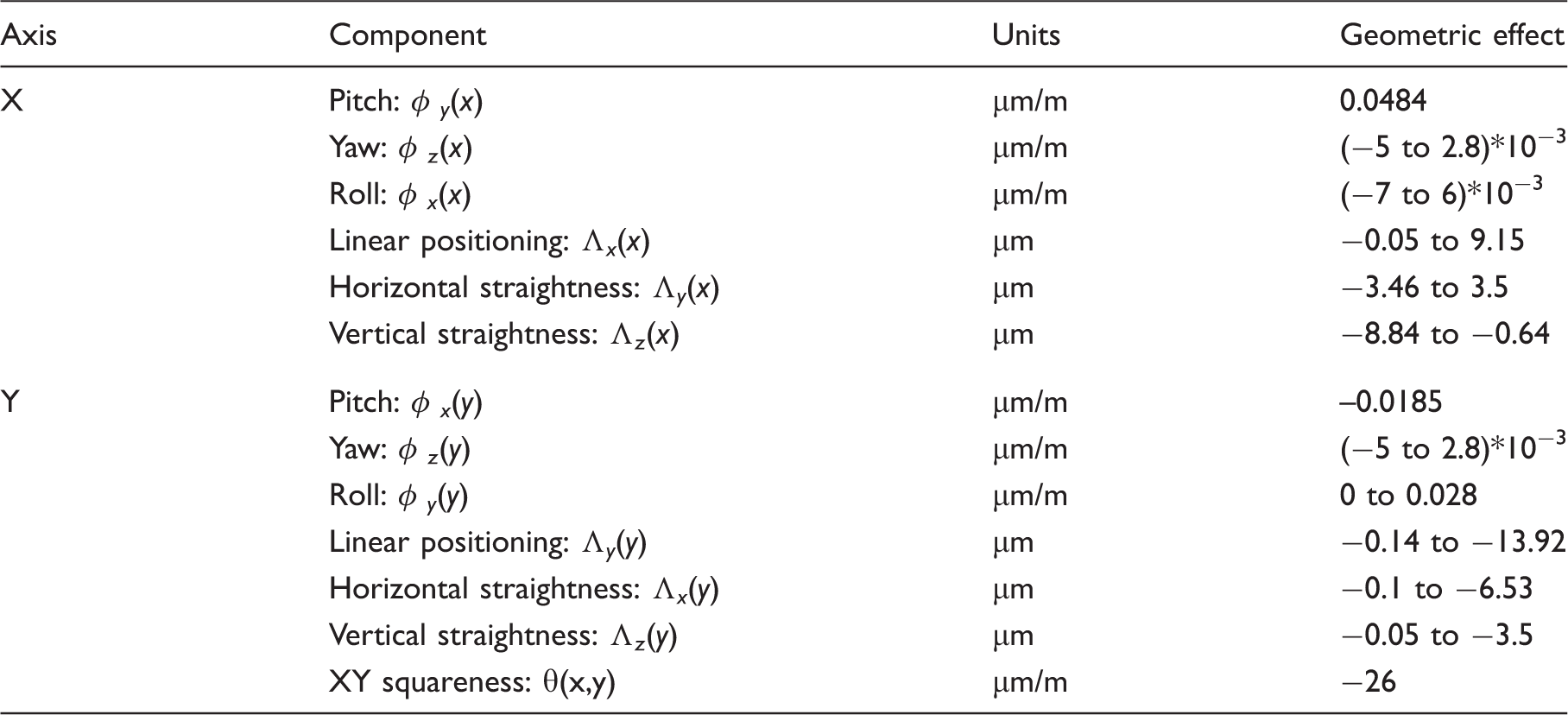
Ford et al. 25 derived algorithms for the real-time correction of time and spatial errors in a similar vertical machining centre configuration. Pre-calibrated geometric errors are included in the form of an error map that is used to correct the control movements over the working zone. Figure 10(b) represents the block diagram for the two-axis model. These errors are measured by using linear interferometers, straight edge, electronic levels, dial gauges, ballbars and granite squares.25–27
Measurements of the geometric and non-rigid errors.
Simulation approach for TLM models
Choice of simulation method
One of the aspects that lead to the study of the TLM method for the modelling of feed drives was the possibility of formulation of comprehensive models which would be implemented in real time. MATLAB28,29 was used as the computational environment where high-level programming and visualisation functions were integrated for modelling, simulation and analysis of dynamic systems. The models were formulated in SIMULINK 30 and then into a program or as block diagrams using the Graphical User Interface (GUI).
SIMULINK contains a large library of pre-defined blocks that supports the modelling of linear and non-linear systems in continuous time, sampled time, or a hybrid of the two. Systems can also be multi-rate, i.e. have different parts that are sampled or updated at different rates. SIMULINK features a tool called Real Time Workshop (RTW), which automatically generates C code from the SIMULINK models to produce platform-specific code.
Simulation method and development
Five SIMULINK multi-rate subsystem blocks, i.e. position controller, velocity controller, current controller, torsional loop and axial loop (the latter two including for mechanical vibrations and non-linearity’s such as backlash and friction forces) were implemented into the software for each axis. The variables interfacing the multi-rate subsystems were implemented in Data Stored Memory Blocks (DSM). A DSM defines a memory region for use by the data store read and data store write blocks. The feature gives access of the memory region to the different sub-systems in order to read from or write to at predetermined designed variable sample rates.
As an example to the approach, implementation of the single-axis model for the test rig in SIMULINK had to deal with the multi-rate requirements (see the Motion controller section): (a) position controller: vref at a rate tp = 3 ms; (b) velocity controller: iqref at a rate tv = 0.6 ms and (c) current controller: edqref at a rate tc = 0.2 ms.
In addition, each PWM signal is composed of seven edq voltages (switching states) calculated according to the expected currents to be induced in the motor. The duration of each edq voltage is specified in multiples of the propagation time for the torsional model (tt). To accomplish this, tt is made equal to the sampling period on the PWM signal (tpwm). The propagation time on the axial model is a sub-multiple of the torsional propagation time as defined by the Castaneda method 9 which describes in detail the synchronisation of the torsional and axial models. These actions result in five multi-rate subsystems per axis which were implemented in software for multi-axis system application.
Model development
The modelling development was carried out according to the following methodology:
The model for the single axis test rig was built in SIMULINK in order to validate the modelling approach. The validation of the model was achieved by comparing simulated results with the experimental data recorded from the controller. Following this step, the single and two axis models for the CNC machine were implemented in SIMULINK taking as a basis the TLM model for the test rig. The x- and y-axes models were validated against experimental data recorded from the controller and the axis drives. The controller's facilities included an integrated oscilloscope and the ability to input stimuli such as PRBS, jerk, and linear/circular interpolation. It also provided an additional capability to perform spectral analysis. The two axis model was validated against experimental data recorded in real time for a ball bar circular test and jerk limited responses (see section on Validation). The models to include for the effect of geometric errors measured with specialised equipment such as laser interferometer, ball-bar, electronic precision levels, precision squares, etc. (Table 3). The simulated results were compared with the measured ones (see section on Validation). Built-in functions on the CNC machine motion controller enabled spectral analysis to be carried out for the optimisation of the position, velocity and current closed loops for each axis. The control frequency characteristics were calculated by entering a PRBS at the set point of each control loop. Four frequency responses were measured, i.e. closed position controller loop, closed velocity controller loop, system and mechanical frequency response. The closed loop responses for the position and velocity controller were analysed and used for the optimisation of their parameters. The control system and mechanical frequency responses were used to set up the parameters for the filters that are used to damp the system resonant frequencies. The data measured were included in the system simulation and used also for the identification of axis drive modal parameters. Other stimuli waveforms were entered to identify parameters suitable for the model such as step (velocity bandwidth overshooting check), triangular (backlash/ dead band), trapezoidal (position gain/coulomb friction) and random white noise/swept sine (resonant frequencies/damping coefficients). The x-axis of the CNC machine was further modified in order to explore the possibility of a real-time implementation for the models. In this regard, the real-time workshop capability of MATLAB/SIMULINK was used to generate a real-time application targeting a RTI-1005 dSPACE environment. The RTI-1005 dSPACE platform was selected because it features the possibility for data logging, control and monitoring of systems in real time.
MATLAB/SIMULINK programs
SIMULINK programs compiled and developed
A bench mark MATLAB/SIMULINK program was compiled and applied to a previously simulated rotor shaft already in the public domain which was then used to evaluate the reduction of mathematical operations and mean square modelling errors when comparing TLM and MTLM techniques (Conclusions section). Single Axis test rig model simulation (see section on TLM method applied to CNC machine tool feed drive) Two axis CNC machine tool model simulation (see section on Implementation of two- axis TLM models to a CNC machine tool) XY geometric calculation in a SIMULINK block. Developed for insertion of measured geometric errors at the machine into the simulated two axis model (see sections on Implementation of two- axis TLM models to a CNC machine tool and Validation).
MATLAB programs compiled and developed for the following
Structure of data for the pulse propagation on the axial model (see Screw shaft axial model section) Parameters and initialisation code for the torsional loop subsystem (see Screw shaft torsional model section) The PWM generating function (see sections on Inverter and motor (electrical) and Motor mechanical equations and coupling) Calculation and nut monitoring blocks (see Screw shaft, nut and table section) Parameters and initialisation code for the axial loop subsystem (see Screw shaft axial model section) Identification of drive modal parameters using the Continuous Wavelet Transform (CWT) for improved performance when compared to other available analysis techniques Automatic modal parameter identification using the CWT Reference signal profiles swept sign, sinusoidal, white noise, jerk, linear interpolation and circular interpolation (for application comparison) Axis block parameters and initialisation code (see section on Motion controller) Calculation of polynomial coefficients for the geometric errors (see section on Implementation of two- axis TLM models to a CNC machine tool) Calculation of the dilation parameters associated with CWT Identification of damping factors and resonant frequencies to be used for axis control system frequency response.
The complexity and detail required for this section is beyond the scope of this publication. To address this issue, we have put all the detail for drive data, measurement methodology, parameter determination, coefficient analysis and a full description of relevant MATLAB/SIMULINK programs online. Most of the detail being contained within the appendices of that report. 9
Validation
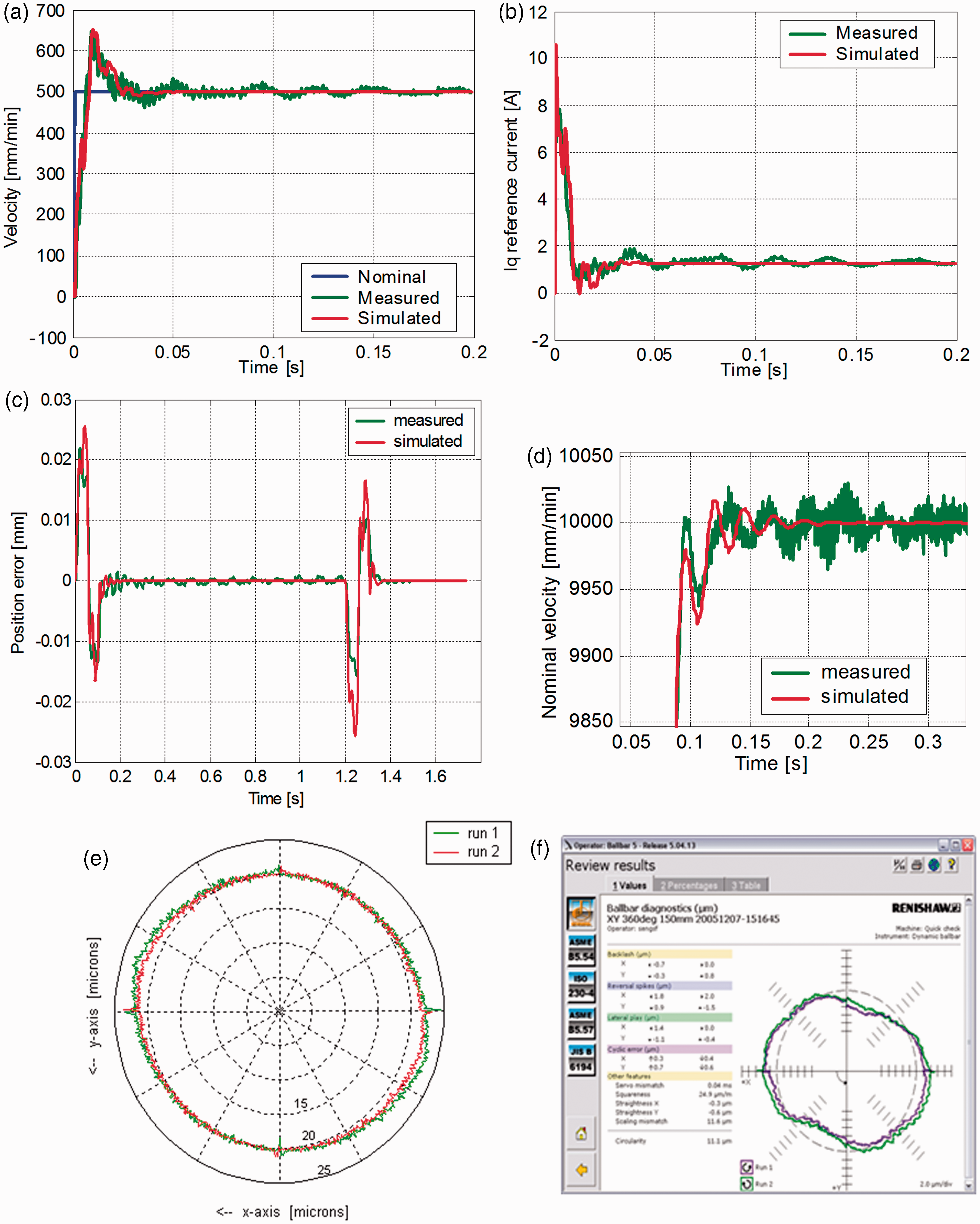
Step velocity stimuli were tested for 500 mm/min (see Figure 11a) and 1000 mm/min where the simulated velocity and current responses (red line) match the machine measured values (green line). A 3% error was achieved in the transient area (0–0.02 s). The % error increases to 5% when the motor reaches constant velocity (Figure 11b). The jerk-limited response was used to verify the performance of the axis drive during acceleration, deceleration and operation at constant velocity. For this purpose, position and velocity responses were measured for different displacements (10, 20, 100, 200, 400, 400 mm) and corresponding feed rates (500, 1000, 5000, 10,000, 20,000 and 40,000 mm/min). Figure 11(c) shows the comparison between measured and simulated position following error for a displacement of 200 mm and a feed rate of 10,000 mm/min. The position versus time measured at the machine and simulated responses matched very well with no significant error but the following error differed minimally by 2 µm at its peak in the acceleration zone and 8 µm at its peak in the deceleration zone. Figure 11(d) shows the comparison between the measured (green line) and simulated (red line) actual velocity signals over the zoom acceleration zone. The same reference position and velocity feed-forward signals (radius 150 mm, feed rate of 1000 mm/min) were used for the circular interpolation in the X-Y plane at the machine and for the validation of the x- and y- axis TLM model responses (i.e. response to sinusoidal and cosinusoidal demands). The two-axis model was simulated and the model position responses were introduced to produce the trace of x against y. The difference between the trace and the circle is illustrated in Figure 11(e) in the form of a circular plot analogous to that measured using a double ball bar. The same sinusoidal stimuli used for the simulation was applied at the machine and the position outputs measured using a Renishaw ball bar system (Figure 11f). An angular overshoot of 180° before and after data capture for a two cycle 360° operation was utilised to minimise uncertainty of test synchronisation. Figure 11(e) plot has an oval shape as a result of the squareness error (−26 µm/m) which is consistent with Figure 11(f). The TLM model shows that the introduction of the geometric errors generates a progressive error deviation when the machine worktable prescribes a circle. The simulated results do not match the machine measurements on the arcs described in the (45–90°) and (135–270°) zones but with sensitivity analysis this could be further improved. The difference may be due to divergences on the straightness measurements for the x-axis. The reversal spikes match closely on both the x- and y-axes. Validation responses comparing TLM model with measured machine. (a) Step velocity response, (b) reference current response to step, (c) position error response jerk-limited input, (d) velocity response to jerk limited input, (e) simulated ball bar trace and (f) measured machine ball bar trace.
Conclusions
A new MTLM stub was developed which improves the convergence and computational processing speed of the original stub algorithm. A reduction of 40% in the number of mathematical operations and almost 35% reduction in the mean square modelling error figures were achieved over the original TLM stub model. Comprehensive transmission line models for the elements of a typical arrangement of a CNC feed drive have been described. All non-linear functions including geometric and load errors have been included as calculated and identified by the measurements undertaken. Equipment such as laser interferometer, ball bar, electronic levels, signal acquisition systems and others were used to obtain parameter data. A TLM model for a CNC single- axis feed drive including a digital controller has been developed and then extended to a two-axis drive of a machining centre including geometric and load errors, thus forming the basis for universal CNC machine tool models. The simulation of the single-axis and two-axis models to various feed rates and displacements including linear and circular interpolation matches well in comparison with the measured response of the machines under study (see Validation section). The application of the MTLM transform and the torsional/axial model’s synchronisation approach to the modelling of single- and two-axis drives led to a real time implementation of the feed drive models. Subsequent work not reported in this paper has shown the feasibility of developing the model for implementation of the two- and three-axis models running in real time. The x-axis of the machine was modified later in order to explore the possibility of a real-time implementation for the models. In this regard, the real time workshop capability of MATLAB/ SIMULINK was used to generate a real-time application targeting a RTI-1005 dSPACE environment. The RTI-1005 dSPACE platform was selected because it features the possibility for data logging, control and monitoring of systems in real time.
Footnotes
Conflict of interest
None declared.
Funding
We acknowledge the financial support from the EPSRC Ref. No: GR/S07827/01 and the collaborating companies and also thank the University of Huddersfield provided additional finance to enable further progress.