Boundary conditions for molecular dynamics simulations of water transport through nanotubes

Abstract

This article compares both new and commonly used boundary conditions for generating pressure-driven water flows through carbon nanotubes in molecular dynamics simulations. Three systems are considered: (1) a finite carbon nanotube membrane with streamwise periodicity and ‘gravity’-type Gaussian forcing, (2) a non-periodic finite carbon nanotube membrane with reservoir pressure control, and (3) an infinite carbon nanotube with periodicity and ‘gravity’-type uniform forcing. Comparison between these focuses on the flow behaviour, in particular the mass flow rate and pressure gradient along the carbon nanotube, as well as the radial distribution of water density inside the carbon nanotube. Similar flow behaviour is observed in both membrane systems, with the level of user input required for such simulations found to be largely dependent on the state controllers selected for use in the reservoirs. While System 1 is simple to implement in common molecular dynamics codes, System 2 is more complicated, and the selection of control parameters is less straightforward. A large pressure difference is required between the water reservoirs in these systems to compensate for large pressure losses sustained at the entrance and exit of the nanotube. Despite a simple set-up and a dramatic increase in computational efficiency, the infinite length carbon nanotube in System 3 does not account for these significant inlet and outlet effects, meaning that a much smaller pressure gradient is required to achieve a specified mass flow rate. The infinite tube set-up also restricts natural flow development along the carbon nanotube due to the explicit control of the fluid. Observation of radial density profiles suggests that this results in over-constraint of the water molecules in the tube.

Introduction

Efficient desalination of sea water is an increasingly important issue, as the World Health Organization estimates that four billion people in 48 countries will not have access to sufficient fresh water by the year 2050. Aligned carbon nanotubes (CNTs) as part of a membrane have been found to possess properties that are potentially of use in filtration and desalination applications. Key characteristics observed are very fast mass flow rates (much faster than is predicted from the Hagen–Poiseuille equation), along with excellent salt rejection capabilities. ¹ Although advances are being made in nanofluid experimental work, there is still significant difficulty in experimental measurements for devices at this scale. ²

Although computationally intensive, non-equilibrium molecular dynamics (MD) simulation has recently been adopted as the numerical procedure of choice for nanoscale fluid dynamics due to its high level of detail and accuracy. Simulation of fluid transport through a CNT using MD requires generation of steady pressure-driven flow, which can be achieved by application of boundary conditions to the flow domain. Various boundary condition configurations exist, each with advantages and disadvantages, and selection often depends on the desired balance between computational efficiency and accurate representation of the physical situation.

There are two common approaches to CNT fluid-transport simulation using MD. The first is to model the CNT as part of a finite membrane in which the CNT is placed between two reservoirs that are set at different hydrostatic pressures. When using this approach, either periodic or non-periodic boundaries can be implemented in the streamwise direction. An existing technique, which uses streamwise periodicity and numerical permeability to generate a streamwise pressure difference across the CNT, is the reflective particle membrane (RPM). ³ This RPM, located at the inlet of the system, controls the number of molecules crossing the inlet boundary in the negative streamwise direction, thereby adjusting the upstream reservoir density. It is however very difficult to control precisely the pressures in both reservoirs, and extensive trial and error is required to achieve a specific pressure difference. A more common technique, which again uses streamwise periodicity, is to apply an external uniform streamwise force to molecules in a region of the upstream reservoir. ⁴

Despite their computational efficiency and simplicity, periodic boundary conditions carry limitations and so non-periodic streamwise boundaries are often applied. One example is the method of self-adjusting plates, ⁵ in which external forcing is applied to plates located at the outer boundaries of the system to achieve a specific pressure in each reservoir. However, as the number of molecules in the simulation is fixed, all molecules will eventually be forced out of the upstream reservoir, effectively ending the simulation. Also using non-periodic boundaries, another recent technique ⁶ sets the upstream system boundary to be a specular-reflective wall, while the downstream boundary deletes molecules upon contact. Upstream pressure control is achieved through proportional-integral-derivative (PID) control feedback, together with adaptive mass-flux control at the inlet to replenish the system, while downstream pressure is controlled using a pressure flux controller.

The second approach to CNT fluid-transport simulation using MD involves modelling only a section of the nanotube and applying streamwise periodicity to create a CNT of effectively infinite length. Although this substantially reduces computational expense, there are concerns that significant inlet and outlet effects are not accounted for.7–9 The most popular method for producing fluid flow in this configuration is to apply an external uniform force to all water molecules in the CNT. This is known as the gravitational field method. ¹⁰

The aim of this paper is to compare several of these techniques in terms of the flow behaviour they produce, their computational efficiency and the required level of user input. Three systems are simulated: a finite CNT membrane with streamwise periodicity and ‘gravity’-type Gaussian forcing, a non-periodic finite CNT membrane with reservoir pressure control, and an infinite CNT with periodicity and ‘gravity’-type uniform forcing.

Simulation methodology

All simulations are performed using OpenFOAM. ¹¹ This software incorporates a parallelised non-equilibrium MD solver, mdFoam,12^–14 written in the research group of the authors. In MD simulations, molecular motion is determined by Newton’s second law. Integration of the equations of motion is implemented using the velocity Verlet scheme with a time step of $1\times {10}^{-15}$ s. The water model chosen is the four-site rigid TIP4P water model. ¹⁵ This consists of a neutral oxygen atom site (O), positive electrostatic point charges of +0.4238e at the two hydrogen sites (H), and a negative electrostatic point charge of −0.8476e at a site M, just above O along the bisector of the HOH angle. Potential interaction between water molecules is represented by a Lennard-Jones (LJ) interaction between oxygen atoms only, using the following parameters: ${\sigma }_{\mathrm{OO}}=3.154$  Å and ${\epsilon }_{\mathrm{OO}}=0.6502\mathrm{kJ}{\mathrm{mol}}^{-1}$ . Similarly, the carbon–water interaction is based only on the carbon–oxygen LJ potential using the following parameters: ${\sigma }_{\mathrm{CO}}=3.19$ Å and ${\epsilon }_{\mathrm{CO}}=0.392\mathrm{kJ}{\mathrm{mol}}^{-1}$ . ¹⁶ Both electrostatic and LJ interactions are smoothly truncated at 1.0 nm.

The type of nanotube used in this work is a (7,7) single-wall CNT with a diameter of 0.96 nm. This CNT has been identified as possessing optimum attributes for desalination; it removes 95% of salt while transporting water at a suitably high flow rate. ¹ To construct a model CNT membrane in MD, the CNT is placed between two perpendicular graphene sheets. To speed up the simulations, both the CNT and graphene sheets are modelled as rigid structures, as previous studies have indicated that this is a fair assumption. ⁹ The CNT has a length of 2.5 nm while the fluid reservoirs have dimensions of $4.4\times 4.4\times 4.4{\mathrm{nm}}^3$ . In all simulations, periodic boundary conditions are implemented in the y- and z-directions, perpendicular to the streamwise x-direction.

When simulating a membrane system, the fluid is controlled within regions of the fluid reservoirs that are far from the entrance and exit of the CNT, ensuring that the flow dynamics inside the CNT are not disturbed. A Berendsen thermostat ¹⁷ is applied to both reservoirs to maintain a constant temperature of 298 K, removing any effects of temperature gradients on the fluid flow. The chosen boundary condition configuration will generate the specified pressure difference between the reservoirs, the magnitude of which will determine the flow rate through the CNT. In reality, industrial filtration processes impose pressure differences of 5–7 MPa across CNT membranes. In MD, however, the non-continuum flow through small diameter CNTs means that measurement of continuum properties requires a large number of samples to eliminate molecular noise, particularly for low streaming velocities. Accurate pressure measurement, performed here using the Irving Kirkwood equation, ¹⁸ requires considerably more statistical samples than density or velocity.^19,20 For the narrow CNTs used here, pressure differences of only 5–7 MPa will produce flow rates much too low for resolving a noise-free signal in MD. Even using state-of-the art processors, the long averaging times that would be required are not currently accessible. In MD simulations, the common solution to this is to increase the pressure drop across the CNT to obtain low-noise results within realistic time-scales.^1,21,22 Accordingly, a pressure difference of 200 MPa is imposed across both membrane systems, with the downstream reservoir maintained at atmospheric conditions. Using such large pressure differences, it is very difficult to make direct comparisons of mass flow rates between MD simulations and experiments. Comparisons are consequently often made through the flow enhancement factor, which is the ratio of the measured flow rate through the CNT to the equivalent hydrodynamic flow rate (calculated using the Hagen–Poiseuille relation). There is, however, variation in reported flow enhancements, possibly due to differences in interaction parameters, water models and boundary conditions.

In both membrane simulations, the reservoirs are initialised with water molecules, after which the CNT is opened and allowed to fill naturally. The development time for this was determined by monitoring the variation of the total number of molecules in the CNT and the average fluid velocity with time; transient effects were deemed to be negligible when these variables reached steady conditions. On reaching steady state conditions, averaging of properties is then performed over a period of 4 ns.

System 1: Finite CNT membrane with streamwise periodicity and Gaussian forcing

Fully periodic boundaries are often employed in MD^23,24 as they enable representation of a large system through simulation of only a small volume. This can significantly reduce the computational expense incurred, meaning larger problem time scales can be achieved with the same computational resources.

The combination of a fixed membrane, streamwise periodicity and streamwise external forcing can generate a specific pressure difference across the CNT, regardless of the chosen form of forcing. Negative pressures are, however, often observed in the downstream reservoir. ²² To mitigate this, density control is implemented in the bulk regions of both reservoirs, ensuring atmospheric conditions in the downstream reservoir while maintaining the desired pressure difference.

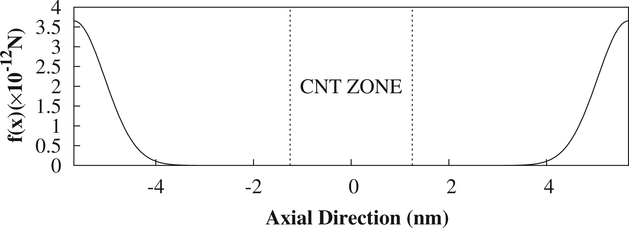
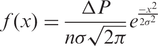
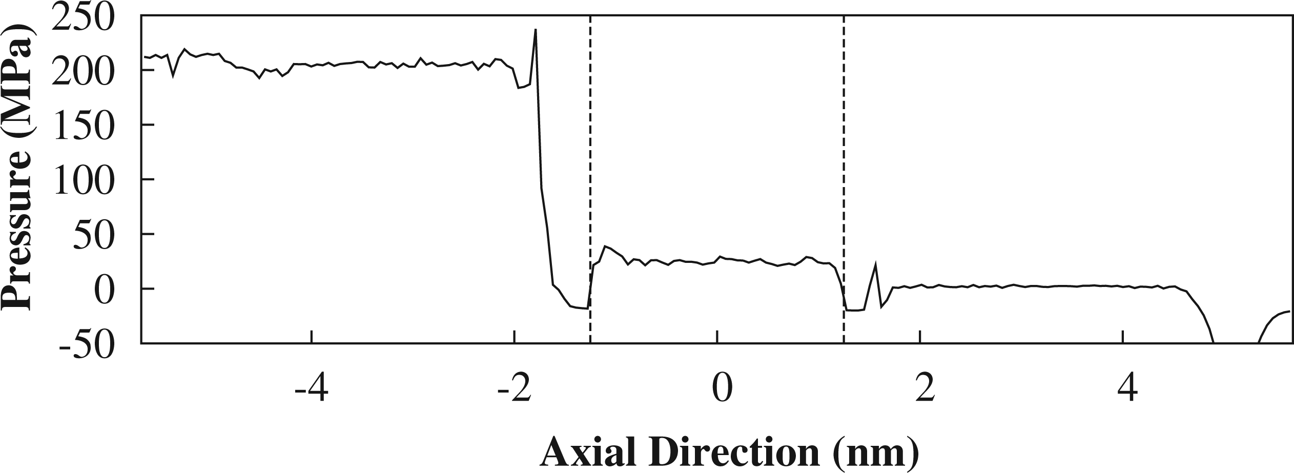
Figure 1 shows a schematic of the simulation domain with Gaussian forcing distributed across both reservoirs. The force exerted on the water molecules varies with the streamwise coordinate through

$f(x)=\frac{\Delta P}{n\sigma \sqrt{2\pi }}{e}^{\frac{-x^2}{2{\sigma }^2}}$

(1)

where $\Delta P$ is the desired pressure difference across the reservoirs, n is the number density in the upstream reservoir and σ is the standard deviation of the Gaussian distribution in the streamwise direction. This forcing function, shown in Figure 2, produces a smooth force variation, unlike a uniform molecular forcing which has step discontinuities. Gaussian forcing improves continuity of fluid properties across the bulk regions of the reservoirs, which can be observed in the pressure profile simulated across the system, shown in Figure 3. Variation of pressure at the streamwise periodic boundaries of the system is gradual and smooth, levelling out to the desired bulk value in each reservoir. The pressure oscillations close to the inlet and outlet of the CNT are caused by physical layering of the molecules close to the membrane. ²⁵

Figure 1.

System 1 simulation domain, with streamwise periodicity and Gaussian forcing.

Figure 2.

Gaussian distribution of streamwise molecular forcing across the domain.

Figure 3.

Resultant axial pressure distribution across System 1.

System 2: Finite CNT membrane with streamwise non-periodicity and reservoir pressure control

Although more computationally intensive than periodic boundaries, non-periodic boundary conditions are necessary to simulate many engineering applications, for example, in systems which require different inlet and outlet conditions/geometries. Hybrid MD-continuum simulations also require non-periodic boundary conditions at the coupling interface.

Implicit pressure control can be achieved through controlling density and temperature to fixed values in both reservoirs ²⁶ and using specular-reflective walls at both boundaries. Although this method is effective, it is sometimes more practical to control pressure directly. This can be achieved using a new boundary condition configuration. ⁶ Upstream pressure is controlled explicitly through a PID feedback loop algorithm that applies an external force over all of the molecules in a user-defined control region. Three separate components of force are summed to create this external force: a proportional term, derivative term and an integral term. Adaptive control of the mass-flux is implemented at the inlet to compensate for any molecules leaving the system. Downstream pressure control is performed using a pressure flux technique ²⁷ so that flow can develop through the nanotube without over-constraint. Non-periodic boundaries are implemented in the form of a specular-reflective wall upstream while the downstream boundary deletes molecules upon contact, creating an open system. 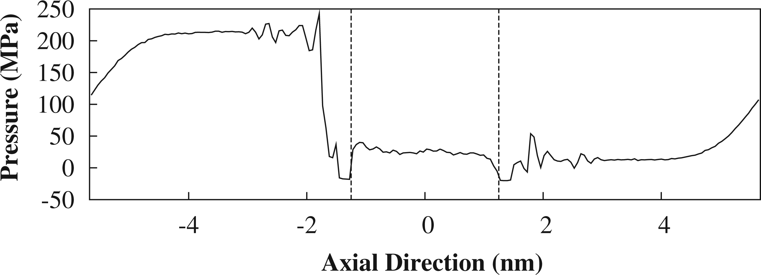²⁸ This in turn automatically regulates the pressure flux forcing. While the pressure flux technique is suitable for control at low pressures, the PID control method is more effective at high pressures. This boundary condition arrangement, summarised in Figure 4, is a fair representation of a physical experimental set-up. The resulting pressure profile across the simulated system is displayed in Figure 5. Unlike in System 1, the boundary conditions implemented here result in small pressure fluctuations within the bulk regions of the fluid reservoirs. A drop in pressure occurs towards the downstream boundary due to deletion of molecules; however, this is not important as it occurs far from the membrane. Again, molecular layering at the inlet and outlet of the CNT causes pressure oscillations close to the membrane.

Figure 4.

System 2 simulation domain, with non-periodic boundaries and pressure control.

Figure 5.

Resultant axial pressure distribution across System 2.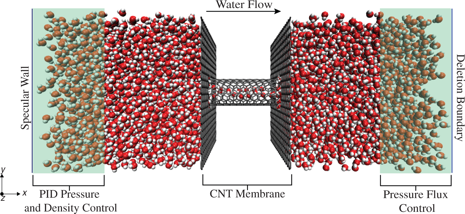

System 3: Infinite CNT with streamwise periodicity and uniform forcing

Modelling a finite length of nanotube and applying streamwise periodicity is equivalent to simulating an infinitely long CNT. While this reduces computational effort, this technique does not account for the entrance and exit effects that are generally present in realistic flows through a finite length CNT. A previous study ⁵ considered the flow of liquid argon through a nanotube and indicated that the influence of these entrance and exit effects on the mass flow rate through the tube can be significant.

In order to imitate a pressure gradient along the CNT, an external ‘gravity’-type force is applied directly to each molecule. To ensure that the behaviour of such a system is comparable to that of a finite membrane system, the number of molecules inside the tube $N_{\mathrm{cnt}}$ remains the same. The magnitude of the external force applied to each molecule, f_g, is chosen to produce an average streaming velocity and mass flow rate approximately equal to that produced in Systems 1 and 2. From this value of f_g, the equivalent pressure gradient along the tube, $\mathrm{dp}/\mathrm{dx}$ , can then be calculated using the following equation (and compared with the pressure difference across the membrane systems to quantify entrance and exit pressure losses)

$\frac{\mathrm{dp}}{\mathrm{dx}}=\frac{\Delta P}{L}=\frac{f_g{N}_{\mathrm{cnt}}}{A_{\mathrm{cs}}L}$

(2)

where $\Delta P$ is the streamwise pressure difference across the CNT and L and $A_{\mathrm{cs}}$ are the length and cross-sectional area of the simulated nanotube, respectively. It is important to note that for smaller CNT diameters, such as the 0.96 nm diameter nanotube used here, there is difficulty in the definition of $A_{\mathrm{cs}}$ due to the structure of the water molecules flowing along the CNT, with no consistency in the literature. ²⁹ The equivalent pressure gradient is dependent on this area, which in this case is assumed equal to the full cross-sectional area of the tube, and hence there is uncertainty regarding its actual value.

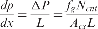
The simulation domain in this case comprises a 2.5 nm length of nanotube, filled with water molecules as shown in Figure 6. Periodic boundaries are applied in the streamwise direction, and a Berendsen thermostat is used directly on the water molecules inside the tube to control the temperature to 298 K.

Figure 6.

System 3 simulation domain, an ‘infinite’ CNT with streamwise periodicity.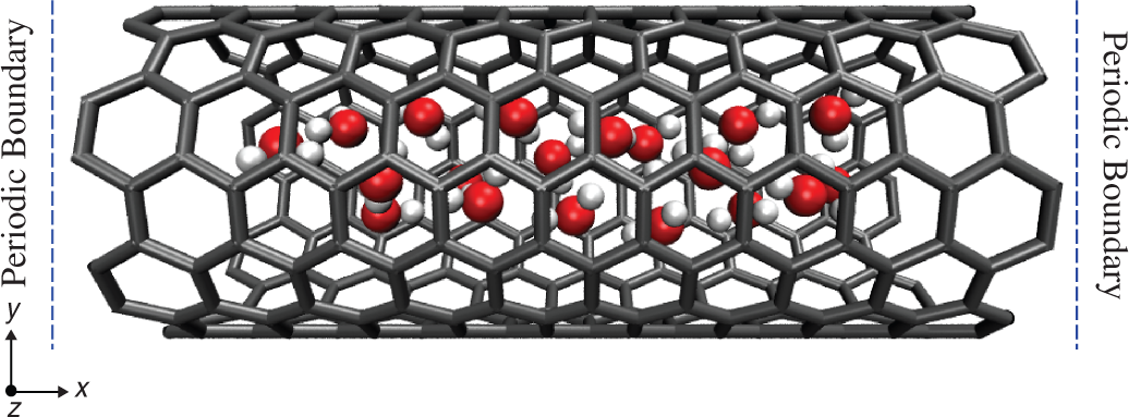

Results and discussion

Inlet and outlet effects

The average streaming velocities U and mass flow rates $\stackrel{·}{m}$ through the channel, calculated over a period of 4 ns, are displayed in Table 1 for Systems 1 and 2. As the flow through the CNT is non-continuum, this mass flow rate is measured by averaging the number of molecules that cross a plane located at the midpoint of the tube over a specified period of time. The flow behaviour in Systems 1 and 2 is seen to be very similar, as is expected given that both systems are essentially simulating the same conditions of flow through a membrane. Slight variations in the flow parameters arise directly from the application of the different boundary condition configurations to the same system, with the configuration of System 2 imposing a higher level of constraint than that of System 1.

Table 1.

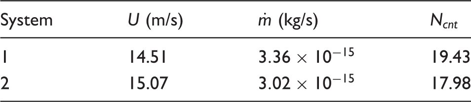
Average values of flow parameters in Systems 1 and 2.

System	U (m/s)	$\stackrel{·}{m}$ (kg/s)	$N_{\mathrm{cnt}}$
1	14.51	$3.36\times {10}^{-15}$	19.43
2	15.07	$3.02\times {10}^{-15}$	17.98

In order to set up the third system, the number of molecules $N_{\mathrm{cnt}}$ inside the CNT must be defined explicitly as it is not possible to fill the CNT naturally. To produce a realistic estimate, simulation of a naturally filled CNT of the same length is required. The average number of molecules inside the channel in Systems 1 and 2, both of which allow the CNT to be filled naturally, is given in Table 1. Taking the average of these values and rounding to the nearest integer, the number of molecules inside the tube in System 3 was set equal to 19. Note that the effect of varying this number by one or two molecules had negligible influence on the final flow results.

By trial and error it was determined that, in order to obtain approximately the same steady-state streaming velocity and mass flow rate as Systems 1 and 2, the force f_g applied to each molecule in System 3 must be $2.39\times {10}^{-14}$ N. The equivalent pressure gradient along this tube is then calculated using equation (2), giving a value of 0.63 MPa over a length of 2.5 nm or 0.252 MPa/nm. This is substantially smaller than the pressure gradient across the membrane systems, which, from Figures 3 and 5, is around 200 MPa over a length of approximately 4 nm or 50 MPa/nm. Therefore, obtaining a specified flow rate along a CNT in a realistic finite membrane system requires a much larger pressure difference across the reservoirs than is suggested by the pressure gradient required for simulating flow in a CNT alone. This higher pressure difference is needed to compensate for significant inlet and outlet effects, which produce large pressure losses at the entrance and exit of the CNT, as observed in Figures 3 and 5. These losses mean that a considerably lower pressure difference is available across the nanotube itself. Entrance and exit effects also manifest themselves as changes in fluid properties at the inlet and outlet. Figure 7 displays axial pressure distributions along the nanotube for both membrane systems, measured using the same number of axial bins over a period of 4 ns.

Figure 7.

Axial pressure distribution along the nanotubes in Systems 1 and 2.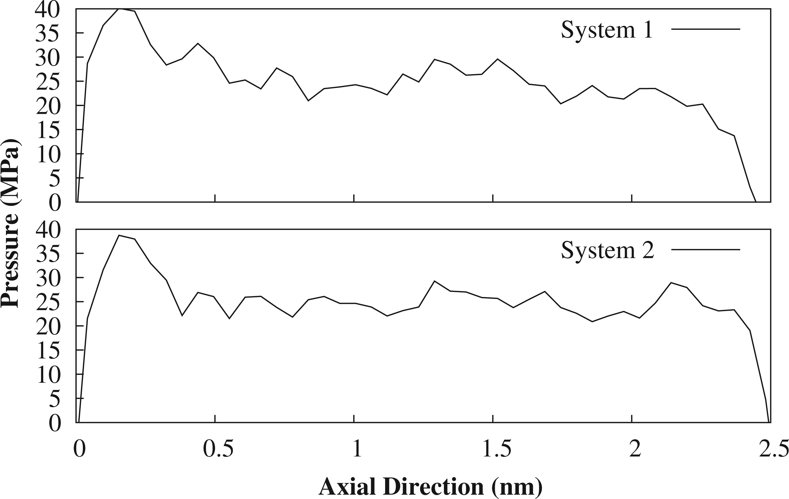

Viscous losses occur at the inlet and outlet of both systems, with a central ‘developed’ region where frictional losses are low. Ignoring the inlet and outlet regions, as in System 3, the pressure gradient along this central region can be approximated. Table 2 presents the pressure gradients along these central regions, from an axial position of 0.5 nm along to 2 nm, for both Systems 1 and 2. It should be noted, however, that, due to the small pressure drop through this region of the CNT, along with the small number of molecules in the CNT and consequent noise associated with pressure measurement, these pressure gradients are subject to considerable uncertainty. Also shown in Table 2 is the equivalent pressure gradient along System 3, in which flow along the entire length of the nanotube can be considered developed. Very low frictional losses in this system result in the mass flow rate along the tube being very sensitive to changes in the magnitude of f_g.

Table 2.

Pressure gradients in the regions of developed flow for all nanotube systems.

System	dp/dx (MPa/nm)
1	0.962
2	0.485
3	0.252

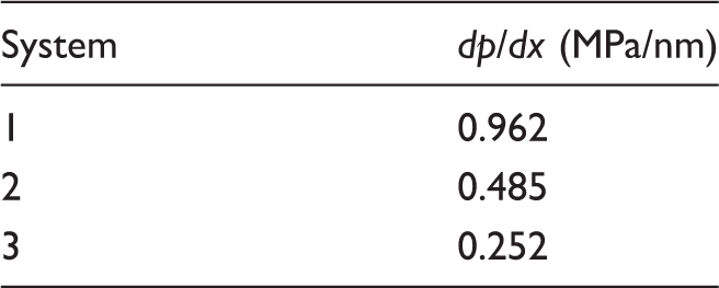
As expected, the pressure gradients in the central regions of Systems 1 and 2 are in much better agreement with the equivalent pressure gradient along the infinite CNT. These simulations therefore verify that, for membrane systems, inlet and outlet pressure losses are very large in comparison to the pressure drop through the CNT itself. Such losses are likely to be less significant in longer CNTs, as the central regions of developed flow extend proportionally with the length of the CNT. ⁶ Other investigations^6,22 have recorded inlet and outlet losses of similar magnitudes to those presented here. Therefore, care must be taken in interpreting any flow rate enhancement from simulations of infinite CNT systems, as the pressure drop required will be considerably smaller than that required across a full membrane simulation for the same flow conditions. While simulation of a finite membrane system is more representative of a physical experimental set-up than simulation of an infinite CNT, the applied pressure differences are very different and so it is difficult to comment on the impact of inlet and outlet effects on real membrane systems. Whether these large external pressure losses are physically realistic or merely an artefact of the MD domain set-up requires further investigation.

Radial profiles inside the CNT

The structure of the molecules flowing along the nanotube can be examined by considering the radial distribution of density, as shown in Figure 8 for each system. Measurement of radial density is performed along an axial distance of 1 nm, centred at the mid-point of the CNT. Dividing the cross-section of the nanotube into 100 cylindrical bins of equal volume, the mass density in each bin is obtained by averaging the mass of water molecules in the bin over time and dividing by its volume.

Figure 8.

Radial water density distributions normalised with the downstream reservoir density.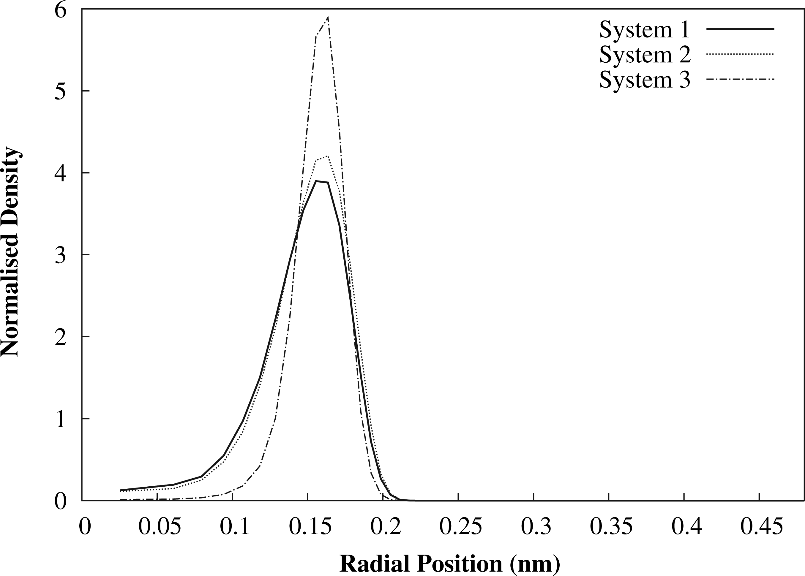

The single-peak structure shown in Figure 8 indicates that the average density profile is annular; the water molecules form one cylindrical shell inside the CNT. This is consistent with previous results.^6,29 These profiles in Figure 8 are normalised using the density of the downstream reservoir in the membrane systems. This is due to the difficulty in expressing the total mass density in the channel, caused by uncertainty in definition of the occupied fluid volume. It is clear from Figure 8 that the peak density occurs at the same radius for all three systems, and so the different boundary conditions do not alter the effective radius of the fluid ring. The peak density in System 3 is however significantly greater than in Systems 1 and 2. It is possible that this is caused by the external forcing placed directly onto the molecules in the tube, resulting in over-constraint of their radial movement. The application of temperature control inside the nanotube could also contribute to this behaviour. Another cause could be the explicit specification of the number of molecules inside the CNT. Therefore, System 3 may not allow for the natural development of the flow structure. Radial profiles of pressure and velocity do not provide additional insight into the flow properties because of the singular ring structure of the water molecules.

Computational efficiency and ease of set-up

Table 3 shows the average execution time for one MD time-step $T_{\Delta t}$ for each system, using a time-step of 1 fs, during an averaging period of 4 ns. Each system is simulated using eight processors (Intel X5570 2.93 GHz).

Table 3.

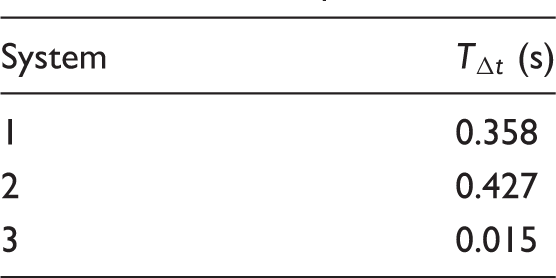
Average execution time for one MD time-step.

System	$T_{\Delta t}$ (s)
1	0.358
2	0.427
3	0.015

Set-up of CNT simulations using MD requires various levels of user input depending on the complexity of the system. Membrane configurations, such as Systems 1 and 2, require enforcing of the desired conditions in both the upstream and downstream reservoirs. For both periodic and non-periodic boundaries, this can be a time-consuming process depending on the fluid state controllers used. For example, using density control to produce a pressure difference across the system can require considerable iteration to achieve the desired pressure values.

Forcing with streamwise periodic boundaries, as in System 1, requires relatively little input to achieve the desired pressure difference; some iteration of the forcing values is sometimes required. Additional density control is, however, required to overcome the negative pressures which appear in the downstream reservoir. This increases set-up time and the amount of user input. Use of Gaussian forcing requires no additional user input above that of uniform forcing. As indicated in Table 3, implementation of periodic boundaries across a finite membrane system results in lower simulation times than for non-periodic boundaries.

Feedback PID pressure control, as used in System 2, drastically reduces user input in comparison with density control, as this allows pressure to be defined explicitly. This method is, however, only suitable for high pressures. Due to the high level of control in this system, it is possible that it could be less stable than other configurations. Although this approach is the most computationally demanding of the three systems, it is more representative of a practical membrane set-up.

Simulation of an infinite nanotube, as in System 3, requires considerably less user input than a membrane system if the aim is to specify a forcing value and monitor the resulting flow behaviour. Aside from temperature control, the user need only specify a value of force to be applied to each molecule. It should be noted, however, that if the aim is to achieve a desired mass flow rate through the system, time-consuming iteration of forcing values is required. As discussed previously, the flow behaviour is very sensitive to the magnitude of the driving force applied due to the very low level of frictional losses in the CNT, and it is not necessarily the case that the response is linear. It can therefore take a considerably long time for this type of system to achieve steady-state conditions. There is also difficulty with setting the number of molecules inside the CNT to an appropriate value: simulation of a naturally filled CNT of the same length may be required to obtain an accurate estimate. As expected, Table 3 indicates that simulation of an infinite CNT significantly increases computational efficiency. This is however at the expense of inlet and outlet effects, as discussed previously.

Conclusions

Various boundary condition configurations for the MD simulation of water transport along CNTs have been compared in terms of the flow behaviour and computational efficiency. In modelling the CNT as part of a finite membrane system, the flow behaviour was found to be independent of streamwise periodicity. While user input is largely dependent on the state controllers used, streamwise periodic boundaries are slightly less computationally demanding than non-periodic boundaries. A combination of periodic boundaries and external forcing can however lead to negative pressure in the downstream reservoir. Additional density control is required to overcome this, increasing simulation time and user input. Use of PID pressure control enables explicit definition of the pressure and hence a low level of user input. Despite a significant improvement in computational efficiency, modelling an infinite length CNT using streamwise periodicity does not account for the important entrance and exit effects that are seen in a more realistic membrane system. To produce specified flow rates through a CNT in a realistic finite system, a considerably larger pressure difference is required across the system reservoirs than that suggested by simulation of an infinite system. This is to compensate for relatively large head losses at the inlet and outlet of the nanotube, significantly lowering the effective pressure difference across the channel. Observation of radial density profiles suggests that explicit control of the fluid inside the infinite nanotube may over-constrain the water molecules. Using a finite membrane system, however, allows for control to be performed in the reservoirs only, resulting in natural flow development throughout the CNT.

Interesting future work might involve simulation of longer CNTs to confirm the trends observed here. Reduction of the computational cost of realistic membrane simulations could be achieved by combining the techniques described in this paper to produce a multiscale hybrid algorithm. Although this work focuses on boundary conditions for water transport along CNTs, these boundary conditions can be applicable to a variety of scenarios which involve transport of matter through a length of nanotube, for example, protein translocation through nanochannels.