
Abstract
Fabric defects in the conventional manufacturing of acoustic panels are detected via manual visual inspections, which are prone to problems due to human errors. Implementing an automated fabric inspection system can improve productivity and increase product quality. In this work, advanced machine learning (ML) techniques for fabric defect detection are reviewed, and two deep learning (DL) models are developed using transfer learning based on pre-trained convolutional neural network (CNN) architectures. The dataset used for this work consists of 1800 images with six different classes, made up of one class of fabric in good condition and five classes of fabric defects. The model design process involves pre-processing of the images, modification of the neural network layers, as well as selection and optimisation of the network’s hyperparameters. The average accuracies of the two CNN models developed in this work, which used the GoogLeNet and the ResNet50 architectures, are 89.84% and 95.45%, respectively, showing statistically significant results. The interpretability of the models is discussed using the Grad-CAM technique. Relevant image acquisition hardware requirements are also put forward for integration with the detection software, which can enable successful deployment of the model for the automated fabric inspection.
Introduction
Background
The manufacturing process of acoustic panels typically consists of panel cutting, panel edging, fabric cutting, fabric lay-up onto panels and packaging. Conventionally, due to the size and the customisation nature of the product, all operations are performed manually, and they would occasionally suffer from human-related problems. Implementing an automated production system following lean methodologies to manufacture acoustic panels would optimise productivity and improve the quality of the products.
This work focuses on automating the fabric inspection process using AI and ML models. Traditionally, fabric quality control is performed via visual inspection by technicians. However, the inspection process is slow and tedious because some types of faults and defects such as broken yarns or multi-nettings are small and can be difficult to identify by the naked eye. 1 Replacing manual inspection with an automated detection system can eliminate human errors caused by oversight and fatigue. 2 An average human inspector can only carry out visual inspections in under 30 min before detection performance declines. 3 Automated fabric inspection processes combining computer vision techniques and AI models have been implemented in the textile industry, and they have outperformed manual inspection in terms of speed, accuracy and consistency. Thus, it is proposed to develop an automated fabric defect detection system by reviewing and applying the relevant technology. In this work, an automated fabric inspection system using advanced ML techniques is developed to detect fabric defects with high accuracy and efficiency. Specifically, deep learning (DL) models with pre-trained convolutional neural network (CNN) architectures are utilised to perform the defect classification.
This work is also a part of an existing initiative to develop a lean and automated production of acoustic panels for the engineering company Soundsorba Ltd, which specialises in the production of acoustic products used in building interiors. This AI detection system is to be implemented in the production line of Soundsorba, replacing the manual fabric inspection.
Related works in fabric defect detection using machine vision and DL CNN
A real-time fabric defect detection system is an industrial application of machine vision technology that has been widely implemented in the textile industry for quality control. Over the past few decades, the progress of machine vision technology has enabled a wide variety of ways to process images and detect fabric defects. These detection methods can be categorised into statistical, spectral, structural, model-based, learning-based or a combination of the above approaches.1,3,4 However, the traditional methods all have their respective weaknesses. For instance, statistical methods such as auto-correlation functions (AF) cannot detect random fabric textures and is sensitive to noise interferences. Model-based Gaussian Markov Random Field (GMRF) method has difficulty in detecting small defects, and the rotation and scaling of the images also affect the detection performance. Spectral and structural methods including local binary pattern (LBP), Fourier transform (FT) and wavelet transform (WT) can only detect defects at the image level and cannot localise the defects. 5 One critical weakness of traditional machine vision technology is that the algorithms are largely fixed designs that are embedded in the vision system software. With traditional algorithms, the image feature parameters must be manually designed. The thresholding of these parameters also requires manual adjustment and tuning. Consequently, they lack the flexibility to adapt to changing conditions of the products and the variety of defects, leading to inconsistent detection results.
In recent years, advanced ML approaches, specifically the use of DL models, are among the most prevalent methods for defect detection due to their reliability, speed and robustness. Some of the earliest research works on fabric defect detection utilising artificial neural networks have been carried out by Tsai et al. 6 and Kumar. 7 Kumar proposed that for real-time defect inspection, a multi-layer feed-forward neural network may be the most optimal approach as it has the fastest model execution speed. For large-scale multiclass image classification applications, CNNs are the most widely used neural network. As opposed to shallow neural network architectures, CNNs are deep neural networks composed of multiple layers, and they use convolution matrixes, or kernels to perform feature extractions. In a CNN, pixels from each image are converted to a featured representation through a series of mathematical operations. By combining multiple layers, complex nonlinear functions can be trained to identify the features or local patterns such as edges within the pixels, which can then map the input images to the classification labels. 8 The hidden layers of CNNs consist of operations such as convolutions and ReLU activations which are for feature detection. A pooling layer is added after each convolutional layer for downsampling to reduce the dimensionality of the convolutional outputs. This helps to generalise the feature map by maintaining the important feature characteristics in the input images but leaving out the fine details that are not as useful. There may be tens or even hundreds of these layers for detecting different features respectively. The classification layers are fully interconnected, and they provide the classification output based on probabilities.
Jing et al. 5 presented a fabric defect detection system based on advanced pre-trained deep CNNs. The model was trained with a two-stage strategy by using the whole image and the local patches of the image. LeNet-5, AlexNet and VGG16 were used as the pre-trained network architectures, and the average accuracies were 93.83%, 94.10% and 96.03%, respectively.
Another study conducted by Sudha and Sujatha 9 utilised two advanced pre-trained CNN architectures, namely, GoogLeNet and AlexNet, for fabric defect detection. The authors used 10 classes of fabric defects and GoogLeNet outperforms AlexNet in the prediction of all the classes. GoogLeNet achieved an average of 99.2% accuracy whereas AlexNet have 89.7%. However, the fabric classes used in this study do not include one that is without defects.
In another work by Jing et al., 10 an improved YOLOv3 framework was used to detect fabric defects on grey and checked cloths in real-time. It is an object detection model such that the localisation of fabric defects over the entire image can be achieved. The model has an accuracy of 97.81% for detecting grey fabric, and 98.24% for latticed fabric. Also, it has an average detection speed of 21.8 fps.
A prototype developed by Blanco 11 at Brunel University London utilised the YOLOv4 object detection model based on the ResNet50 architecture for fabric defect detection. Soundsorba also provided fabric samples for the creation of the image dataset, which contains four classes: ‘oil stain’, ‘hole’, ‘multiple netting’ and ‘no defect’, and there is a total of 903 images. The model can detect images with fabric defects and the accuracy is 88.2%. However, it could not detect ‘no defect’ fabric. The average precision is only 39.5% for the whole test data.
This work is a continuation of Blanco’s ML model development. However, a different design approach is taken such that the model can detect good-condition fabrics, and this is explained in the Design Considerations section. Then, the Results and Analysis section discusses the performances and the explainability of the AI models. It is followed by the Limitations of the Work section discussing the insights gained from the results, and why the model failed to make a correct prediction in certain instances. The Conclusions section at the end provides a summary and suggests ways of improvement for the AI models developed in this work.
Methods
Design considerations
This section presents the design considerations before building the AI model. The task is defined based on the data gathered through observations on the manufacturing floor:
The fabric images should be acquired by an automated fabric inspection machine with a good quality camera and lens, and with an optimal lighting setup.
The overwhelming majority of the actual fabric images acquired will be in good condition and without defects.
The sizes of the faults and defects are extremely small relative to the overall size of the fabric.
As shown in Figure 1, the smallest ink stain or dirt contamination visible is approximately 0.5 mm in size. Accordingly, after image processing, the image resolution must be at least 0.5 mm/pixel or less for the ink stain spots to remain visible.
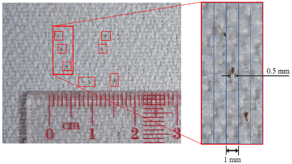
Dimensions of a group of ink stains visible on white fabric.
For this study, the model will apply transfer learning by using pre-trained networks. For most pre-trained CNNs such as GoogLeNet and ResNet50, the input images are rescaled to 224 × 224 pixels. Therefore, the field of view (FOV) of the fabric images feeding into the neural network should be no greater than 112 mm × 112 mm, as illustrated in Figure 2. This can be done by selecting an optimal focal length for the camera lens. An alternative method is to first capture the image on a larger FOV. Then, the image can be cropped to the required size for image processing. If the original image is captured with low resolutions, the compressed image would not be able to retain the information of fabric defects. The shutter speed of the camera in the optics system should at least match the moving speed of the tested sample, in order to avoid blurring and affect the quality of the images acquired.
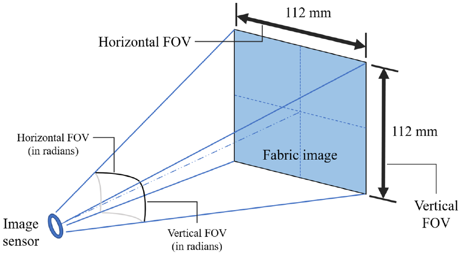
Requirement of image FOV.
CNNs can be applied to tackle two types of computer vision tasks, namely, ‘image classification’ and ‘object detection’. The former is performed at the image level, whereas the latter is performed at the object level with bounding boxes around the indicated objects for annotation. As stated in the previous section, most fabric images will be defect-free, which means no bounding boxes can be created in the image. Hence, the DL model is built to perform the annotation and classification at the image level. The two major classes are ‘defect’ and ‘no defect’. The images with fabric defects are further sub-categorised into their corresponding defect types.
Two CNN models based on transfer learning are developed using MATLAB version R2022a with the necessary toolboxes installed. The models are run on a NVIDIA GeForce RTX 3050Ti GPU, and an AMD Ryzen 7 5800H CPU, with 16 GB (3200 MHz) of RAM.
Fabric image dataset
For this study, the fabrics are provided by Soundsorba with five types of defects used for acoustic panel manufacturing. The fabrics are in assorted colours and with different knitting patterns.
Figure 3 shows examples of each type of defect and Table 1 lists the class proportions.
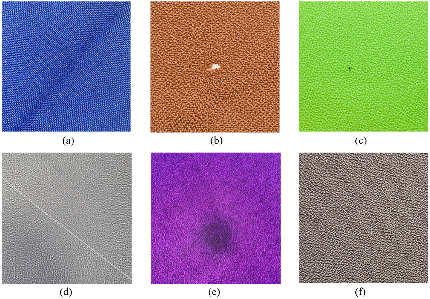
Examples of the six classes of fabric in the dataset: (a) crease, (b) hole, (c) ink stain, (d) multiple netting, (e) oil stain and (f) no defect.
The proportion for each class in the dataset.
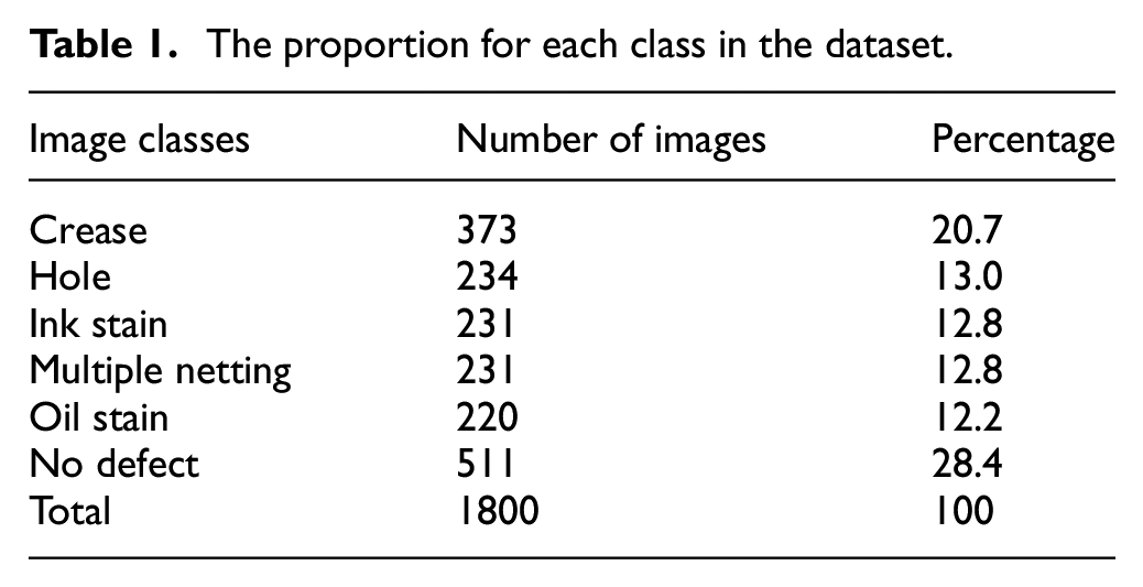
The image dataset is split into training, validation and testing. The most common train-test split ratio for ML models is 80:20. Similarly, in this design, the authors used 20% of the dataset for testing, while 65% of the dataset is for training, and 15% for validation.
Image pre-processing and augmentation
An image data augmenter is created to perform the image pre-processing and augmentation. The image augmentations applied are random rotation from 0° to 360°, as well as random reflection on the x-axis and y-axis, as depicted in Figure 4. Randomised augmentation helps to train the network to be invariant to distortions in the image data and prevents it from memorising the dataset and overfitting. Therefore, the augmentation is only applied to the training dataset. Also, all images are rescaled to 224 × 224 pixels to match the size of the input layer.
Preview of the random transformations on the augmented training dataset.
Transfer learning using pre-trained networks
Given the available resources (the computational hardware to train the network, and the number of images for training), transfer learning has been used to develop the model based on the pre-trained CNN architectures. It is also noticed that with more time and resources, custom-made networks similar to those by Moore et al. 12 have demonstrated the ability to achieve comparable and even higher accuracies on failure mode and defect classifications than the model based on the pre-trained networks.
Based on the literature review, GoogLeNet and ResNet50 are chosen. LeNet and AlexNet are not chosen due to the relatively low performances shown in the studies by Jing et al. and Sudha and Sujatha, and VGG16 architecture is not chosen because it is too computationally intensive for the available hardware resources to handle, as the network contains more than 130 million trainable parameters.
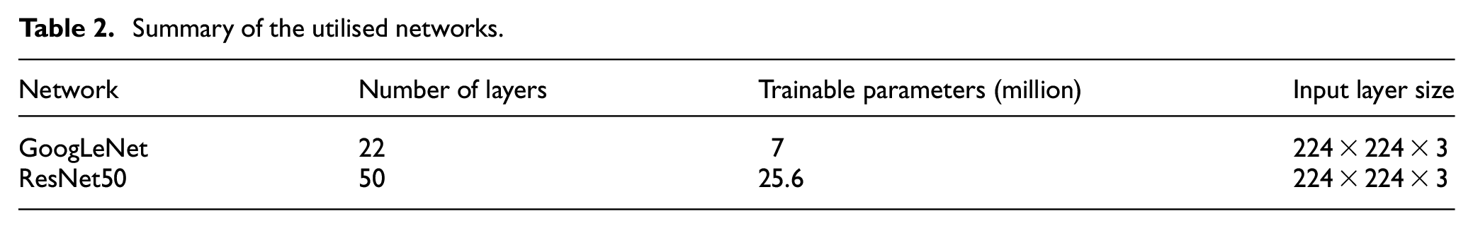
GoogLeNet is a 22-layer deep CNN developed by researchers at Google. 13 ResNet50 has 50 layers, and it is a variant of the deep residual network (ResNet) model developed by He et al. 14 based on the residual learning technique. Both networks were trained on the ImageNet dataset which contains over 15 million labelled images. 15 GoogLeNet uses inception modules that are based on several small convolutions of different weight filter sizes (1 × 1, 3 × 3 and 5 × 5) at the same level for feature extraction. On the other hand, the residual modules in ResNet50 are constructed to solve the vanishing gradient and degradation problem that arises from deeper networks with a single convolution per layer. By comparison, the network structure of GoogLeNet is wider, but ResNet50 is deeper. Both networks each have 1000 output classes, whereas in the fabric image dataset there are only six classes. Subsequently, the final layers of both networks are modified, including the fully connected layer and the classification layer (Table 2).
Summary of the utilised networks.
Hyperparameters of the model
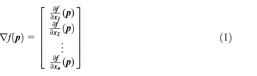
The process of building CNN models involves tuning their hyperparameters. A suitable optimisation algorithm must also be selected when building the model. Gradient descent is the fundamental optimisation algorithm of neural networks by iteratively minimising the gradients of the loss functions during the back-propagation learning of the network. The gradient for an n-dimension multivariate function f(x) at a given point
Then, the next parameter vector point (

The iterations are repeated until the convergence of the local minima, this approach is known as batch gradient descent. Typically, stochastic gradient descent (SGD) or mini-batch gradient descent are performed for their enhanced efficiency because most deep neural networks are handling an exceedingly large dataset.
In this experimental design, the optimisation algorithm chosen is the Adam (Adaptive Moment estimation) algorithm because it combines the advantages of several SGD variants including Adaptive Gradient (AdaGrad) and Root-mean-square Propagation (RMSProp) algorithms. First introduced in 2014 by Kingma and Ba 16 from OpenAI, Adam is an SGD algorithm that uses parameter update with momentum terms that are similar to RMSProp. First, the moving average of both the parameter gradients and their squared values are computed:


where
Then, the parameter vector updates by using the gradient momentums, with
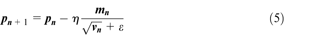
This momentum scaling can help the learning step to escape local minima and plateau regions and to reach the global minimum of the loss function.
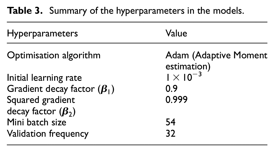
The hyperparameters of the models are fine-tuned during the experimental design and they are described in Table 3. For a fair comparison between the utilised networks, the same hyperparameters are used, except for the number of epochs. Since different network architectures have different training efficiencies, the number of epochs should be optimised based on each network respectively to avoid undertraining or overtraining. After fine-tuning, the optimal number of epochs for the training of GoogLeNet is set to 36. For ResNet50, it is set to 20 epochs. The order of the testing dataset is shuffled after each epoch of training to reduce systematic bias.
Summary of the hyperparameters in the models.
Results and discussions
Model performance
Since the procedure of splitting the dataset into training and testing is done randomly, it is difficult to ensure the sets are truly representative of the different classes in the dataset. To reduce random errors, the training and testing for each pre-trained network are repeated five times.
The performances of the trained model using GoogLeNet and ResNet50 are shown in Figures 5 and 6. As shown in Figure 5, on average, the ResNet50 model took more than double the amount of time to complete the training. The average accuracy of the trained model using the GoogLeNet architecture is 89.84%. Due to the imbalance in the multi-class dataset, the weighted averages of the precision, recall and F-score are calculated according to the proportions of classes. The confusion matrix of the test results for the second repetition (89.17% accuracy) is illustrated in Figure 7. The ‘crease’ class has the lowest F-score (0.8000) and lowest precision (0.7529), indicating a high false positive prediction rate.
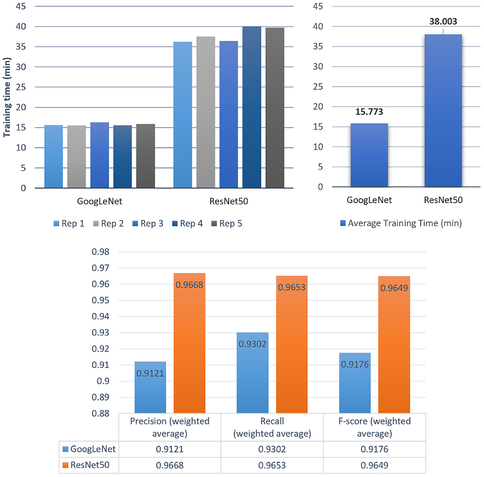
Training and test performance for both models.
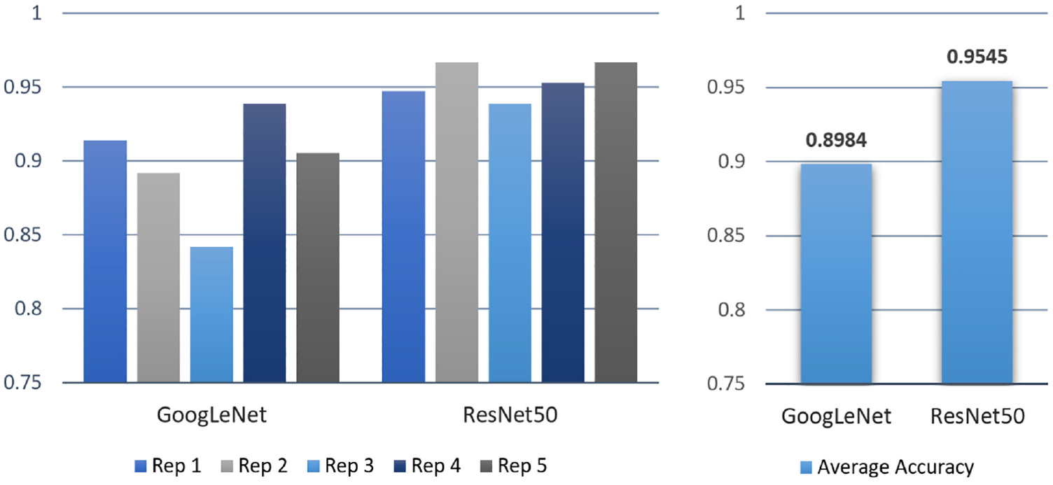
Test accuracies across five repetitions for both models.
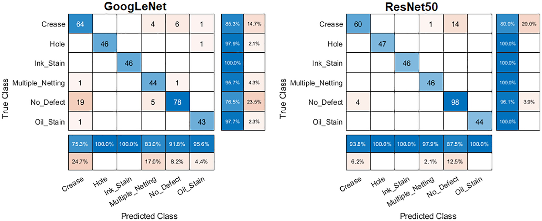
Confusion matrices of the test results.
For the second model using the ResNet50 architecture, the average accuracy obtained is 95.45%. The confusion matrix for the first replication (94.72% accuracy) is also given in Figure 7. Both the GoogLeNet and the ResNet50 model have achieved 100% correct classification for the ‘ink stain’ class. The ‘hole’ and ‘oil stain’ classes have also been predicted with 100% accuracy by the ResNet50 model. The ‘crease’ class has the lowest prediction performance in terms of recall.
The average time for the models to predict a typical fabric image is within seconds. When the system is deployed in an industrial application, more powerful hardware can be utilised, and the prediction speed can be further increased.
A two-tailed independent samples t-test is performed to determine whether the difference in the average accuracy is statistically significant or is simply caused by random variations. It is assumed that both sets of model test results follow the normal distribution with equal variances, because the dataset-splitting procedures are randomised and are done independently for each repetition.
The accuracy values of the five repetitions for GoogLeNet are Y A ∼ N(μA, σA2), and the accuracy values for ResNet50 are Y B ∼ N(μB, σB2), on the assumption that σA and σB are unknown but σA2 = σB2. The hypotheses are formulated as below:
H 0 (null hypothesis): μA−μB = 0 (there is no difference in the average accuracy between the two models)
H 1 (alternative hypothesis): μA−μB ≠ 0 (there is a statistically significant difference, and a two-tailed test is performed)
The significant level α is chosen to be 0.05. Then, the t-value can be calculated according to H0:
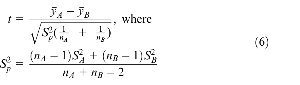
which is computed to be
The degree of freedom is
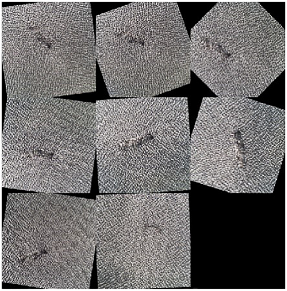
To further investigate the performance of the networks, the incorrectly classified images from the testing sets are selected for checking. Three examples are chosen for comparison, the first is an incorrect prediction of defective fabric, while the second is a correct prediction of defective fabric, and the third is a correct prediction of non-defective fabric. From the confusion matrices, the images with the ‘crease’ class produced relatively poor prediction results. The first example shown in the top image in Figure 8 depicts a piece of grey fabric with a crease on the fabric located diagonally across the image, resulting in a difference in the contrast level. However, the model predicted it as ‘no defect’.
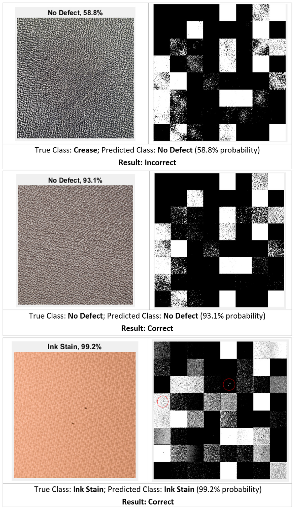
Comparison between three classified images and their activated feature maps.
The activated feature maps of the batch normalisation layer after the first convolution layer are visualised for comparison between the images. Dark pixels are negative weights and white pixels are positive weights. The second image shows a correctly classified, defect-free fabric image. Both images have produced a similar activation output after passing through the first convolution layer for feature extraction, which could explain why the model is struggling to differentiate between the image classes of ‘crease’ and ‘no defect’.
Both models have produced 100% correct predictions on ink-stained fabric. The feature map of the bottom image in Figure 8 shows that the stain features in the input image have already been activated at the first convolution layer. The red circles on the feature map highlighted two noticeable activations of the extracted features, which represent the ink stains.
Interpretability of the CNN models
It is worthwhile to explore what features the hidden layers of the CNN models have learned from the fabric images. This can be done via saliency maps, in which the regions of interest are highlighted to show where in the images the AI models ‘look for’ to make a prediction. The saliency maps are produced using the Gradient-weighted Class Activation Mapping (Grad-CAM) technique. Grad-CAM uses the global average pooled gradients of the output class score (
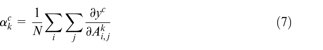
where
Figure 9 shows the images of different fabric defect classes and their corresponding Grad-CAM maps. For holes, ink stains and oil stains, the highlighted regions are directly on the location of the defects because of their inherent small size. It can also be seen that for fabric with creases, the network focused on the shadow of the folds. This means the shadow is the main feature that the network has learned to classify creases. Another interesting finding is that when the input image does not contain any defect, the network would look at the whole image to search for features of fabric defect to make its decision, as evident by the large area of the image being highlighted in the Grad-CAM map.
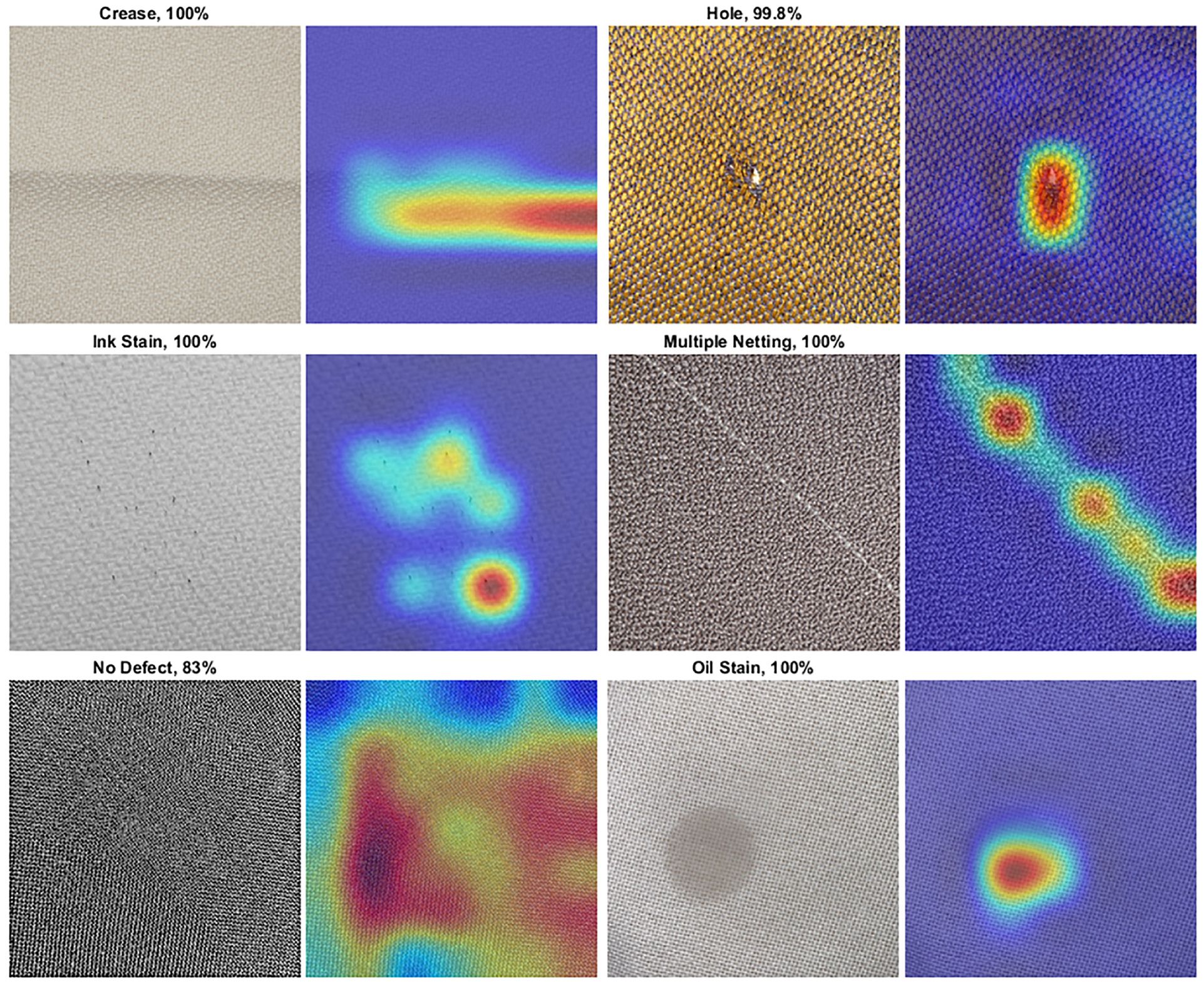
Grad-CAM maps of the different fabric defect classes.
Limitations of the work
The investigation of the test images and their feature maps has shown that both models struggled to differentiate the ‘crease’ and ‘no defect’ classes. The reason could be the features or patterns of creases caused by folding or pressing are not as prominent as the other defects such as ink stains and holes. It is also found that some images with no defect have a slightly noticeable difference in the contrast level, which appears to be caused by the uneven lighting during image capturing.
Moreover, performing classification on the whole image means the model can only produce a single class prediction result. The model cannot perform well if there is more than one type of defect existing in the image, such as the one depicted in Figure 10 that has a crease on the bottom-right (red circle), and multiple netting on the top-left (red rectangle). This would be a rare case scenario, but it should still be considered in future work. Consequently, after running the CNN model to perform image-level classification, the images can be fed into an R-CNN or a YOLO object detector to perform defect localisation.
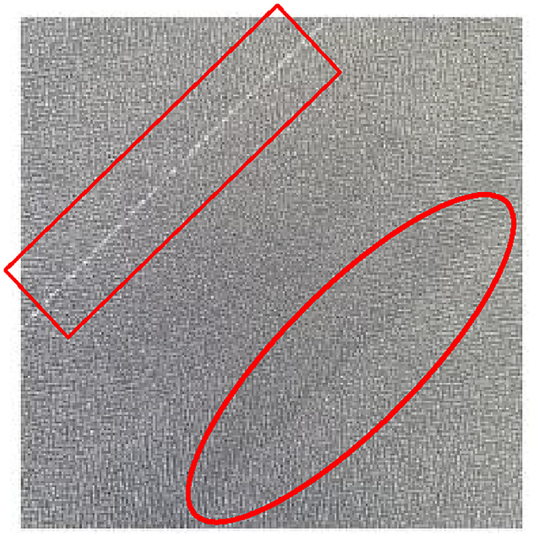
A fabric image containing two defect types.
Conclusions
This project developed two DL models which utilised GoogLeNet and ResNet50, two state-of-the-art pre-trained CNN architectures for the classification of fabric faults and defects. The models are trained on a dataset containing 1800 images of various coloured fabrics with and without defects. The ResNet50 model has obtained superior results in the classification performance with over 95% average accuracy and a weighted average F-score of over 96%. It is also more reliable and robust as it produced a smaller sample standard deviation of the accuracy values when compared to the GoogLeNet model (1.22% vs 3.60%).
The CNN models developed in this work can be readily deployed for industrial applications. Further improvement can be implemented regarding the hardware design of the image acquisition system, as noted in the previous section that the uneven lighting when capturing the images has negatively affected the model performance. The images in this project are captured with the aid of a camera flashlight, which can be improved with a ring light or symmetric side lights with equal luminosity around the camera, as well as a back panel lighting placed under the fabric. This should help eliminate any contrast level differences in the images caused by uneven lighting, so that the network will be performing feature extractions on good-quality images. It is also possible to further improve the design and training of the CNNs, for example, through customising loss functions in the neural network.
Footnotes
Declaration of conflicting interests
The author(s) declared no potential conflicts of interest with respect to the research, authorship, and/or publication of this article.
Funding
The author(s) disclosed receipt of the following financial support for the research, authorship, and/or publication of this article: The work is partially supported by Innovate UK (KTP 12273). Some fabric defect samples are provided by Marian Saricky and Munir Hussain at Soundsorba Ltd.