Sage Journals: Discover world-class research

Abstract

Titanium alloys are extensively employed in machining to produce high-value components, where surface roughness is crucial for their functionality. In this study, the roughness of Ti6Al4V and Ti6Al7Nb turned surfaces was analysed. The goal was to compare the alloy’s roughness behaviour when machined under the same conditions. Therefore, hypothesis testing was performed to assess the equality of the expected values and population median. It was found that, for some parameters, the mean (R_zI, R_t) and median (R_q, R_zD, P_t) roughness was statistically different when changing alloys. However, for others, it did not present a significant difference, in terms of mean (R_mD, R_p) and median (R_a, R_pm). Consequently, a relevant insight from this study was that the phenomenon interpretation was affected by roughness parameter selection. On the other hand, as expected, the feed rate played a critical role in roughness control. It was observed that Ti6Al7Nb had a smoother topography (R_a was 0.15 ± 0.01 μm and 0.62 ± 0.04 μm) than Ti6Al4V (0.31 ± 0.02 μm and 0.67 ± 0.03 μm) at 0.05 and 0.15 mm/rev. Yet, at 0.1 mm/rev, this behaviour changed, as Ti6Al4V had a smoother surface (R_a was 0.40 ± 0.02 μm) than Ti6Al7Nb (R_a was 0.51 ± 0.03 μm). Finally, the multi-optimization indicated that a low feed rate (0.05 mm/rev) and medium (60 m/min) and high (90 m/min) cutting speed led to lower roughness and higher material removal rate for turning Ti6Al7Nb and Ti6Al7V, respectively. The insights from this study may have a practical application in the manufacturing and quality control of biomedical components.

Keywords

Ti6Al7Nb Ti6Al4V turning surface roughness statistical inference

Introduction

Although α + β Ti6Al4V alloy was the number one choice for manufacturing the first generation of titanium implants,¹ researchers found that long-term exposure to Vanadium was correlated with the development of Alzheimer’s disease.² Therefore, other Ti-alloys, such as Ti6Al7Nb, have been preferred for producing implants since they reduce unwanted interactions with the human body. This is achieved without compromising other thermo-mechanical properties that make Ti-alloys suitable biomaterials, including corrosion resistance, good strength-to-density ratio and low elasticity modulus.³

If, on the one hand, the Ti6Al7Nb alloy is more biocompatible, on the other, the number of studies reporting its machinability is still scarce compared to the traditional Ti6Al4V alloy. Nonetheless, relevant contributions were found, including Sun et al.,⁴ that applied liquid nitrogen in Ti6Al7Nb turning and observed an improvement in the surface hardness and finish compared to dry and flooded cooling. Furthermore, Lauro et al.⁵ conducted a very thorough study in Ti6Al7Nb dry micro turning and assessed several responses that characterize the machinability, including machining forces, cutting temperature, chip compression ratio, specific cutting energy and friction coefficient at the rake face. The same authors⁶ performed similar tests with minimum quantity lubrication (MQL) and observed worse surface roughness for MQL conditions due to higher chip adherence (R_a <0.2 μm for dry, and R_a <0.3 μm for MQL). Nonetheless, MQL improved the burr formation by avoiding the growth of a build-up edge. The works described above are praiseworthy as they are among the few describing the effect of the lubrication in the surface state of Ti6Al7Nb.

Reports comparing the two α + β Ti-alloys were also found, including, Fellah et al.,⁷ which noticed, through tribological tests, that the wear resistance of Ti6Al7Nb was lower than Ti6Al4V. More recently, a similar trend was observed by Almeida et al.⁸ To explain the findings, the authors evaluated the topography of worn Ti-alloys surfaces, with reconstruction by extended depth-of-focus, as well as a fractal dimension analysis. Variations in β phase distribution of the Ti-alloys were pointed-out as one of the reasons for the distinct topographical and wear behaviour. A concern that can be drawn from these reports is that Ti6Al7Nb surfaces potentially release more debris in the human body than Ti6Al4V. This, in turn, highlights the relevance of investigating effective machining strategies that promote Ti6Al7Nb smooth surfaces, thereby reducing its potential for debris release.

Furthermore, high-quality surface texture enhances the natural anti-corrosive properties of Ti-alloys, as reported by Avinash and Kumar.⁹ Their findings implied that, in contrast to Ti6Al4V, Ti6Al7Nb surfaces presented a lower corrosion rate. This behaviour was attributed to the greater resistance of dioxide titanium film formed in the presence of Nb elements. However, before the corrosion tests, the roughness evaluation pointed to smoother Ti6Al7Nb surfaces (R_a: 0.15–1.73 μm), rather than Ti6Al4V (R_a: 0.36–1.87 μm). Undoubtedly, this aided in the improvement of the anticorrosion properties of Ti6Al7Nb.

While the previous work,⁹ suggested a better surface finish in Ti6Al7Nb micro-milled surfaces, reports for turning^10,11 showed the opposite trend. Nevertheless, Mello et al.¹¹ found that the turning conditions required to achieve the same (and optimal) surface roughness in both alloys were identical, indicating that they exhibit similar machinability. An analogous inference was found in Filho et al.,¹² as the optimal machining conditions for minimum specific cutting energy for both alloys were the same.

A key point to consider is that while the surfaces may have similar roughness, they can have distinct textures and chemical element distributions, as shown in Carvalho et al.¹³ Indeed, it was found, with an innovative correlative microscopy technique, that variations in the process conditions lead to the formation of clusters of vanadium in feed mark regions of Ti6Al4V surfaces. These heterogeneities were not noted in Ti6Al7Nb surfaces. These insights are particularly pertinent to avoid undesirable interactions between surfaces and the human body.

Thus, the concept of surface integrity is very broad, as it includes topographical, microstructural and mechanical aspects. Yet, the surface finish is undoubtedly one of the key aspects in the manufacturing of functional surfaces, as it accounts for the waviness and micro geometric deviations, namely, the surface roughness. In machining, the latter refers to the irregularities resulting from the interaction between the tool and the material and depends, among other factors, on the process conditions, including cutting speed, feed rate, stiffness of the machine tool, tool nose radius, used of metalworking fluids and others.¹⁴ As irregularities (groves and valleys) induce stress concentrations in the surface, higher wear rate, reduced fatigue resistance and a higher tendency for crack propagation may lead to component failure if surface roughness is not accounted for.¹⁵

Besides, for hard tissue replacements, including joints and dental implants, the surface roughness impacts the structural and functional bonding between the implant and the bone, known as osseointegration.¹⁶ For dental implants, turning and threading operations typically provide a smooth surface with an arithmetic average deviation of the roughness profile (R_a) between 0.3 and 0.6 μm.¹⁷ Nevertheless, many available solutions endured multiple surface modifications, such as abrasion, etching, blasting and coatings to increase the roughness.^16,17 Indeed, a R_a ranging between 0.79 and 2.89 μm was observed by Nicolas-Silvente et al.¹⁶ when assessing off-the-shelf dental implants. It seems that, compared to smoother implants (R_a <1 μm), a certain degree of roughness, preferably between 1 and 2 μm, improves the proliferation and attachment of bone cells, as well as the bone-to-implant contact. Still, as discussed in Jordana et al.,¹⁸ the risk of periimplantitis (inflammation around the implant) intensifies with increasing roughness (R_a >1.2 μm).

On the other hand, for articulating components, such as the femoral head, a R_a below 0.05 μm is required (ISO 7206-2: 2011/AMD 1:2016) to avoid particle generation due to excessive wear.¹⁹ This finish cannot be achieved solely through machining but rather requires grinding and polishing operations. Nevertheless, the better the finish provided by machining, the less time is required for these operations.

To assess surfaces roughness 2D and 3D methods can be used. 2D techniques include stylus profilometry, while 3D technology consists of optical interferometry (3D profilometers),²⁰ confocal²¹ and atomic force microscopy.²² Besides, roughness parameters can be classified as 3D when determined for an area of the surface instead of a line (2D).²³ Due to their capacity to inspect a wider area, thus having higher statistical significance, 3D parameters gained recognition for evaluating heterogeneous rough textures, such as those found in additive manufacturing surfaces.^24,25 Furthermore, as 3D inspection entails additional cost and technical requirements, 2D profilometry is frequently sufficient for analysing well-understood components and processes, such as homogenous surfaces produced by machining. Also, the many decades of data and experience with 2D roughness measurements make 2D profilometry a well-established technique known to academics and industrials. Indeed, contact profilometry has worldwide traceability, as many finish standards used by the industry were defined using it.¹⁹ Other advantages of 2D profilometry include portability, flexibility in measuring small and large workpieces and the capacity to assess inside bores.

From all the 2D roughness parameters described in the state-of-the-art, the arithmetic average deviation of the roughness profile (R_a) is the most acknowledged by the industry and academia.²⁶ Nevertheless, several authors agreed that for some components, the definition of the surface state through R_a is simplistic, as it overlooks the peak and valley distribution throughout the profile.^27,28 The same happens with the root mean square of the surface roughness (Rq). Indeed, surfaces with the same R_a or R_q can vary widely in their surface topology and, therefore, diverge widely in performance.²⁹ Still, R_q is more sensitive to peaks and valleys than R_a since the amplitudes are squared.²³

Another parameter commonly used to describe the machined surface finish is the peak-to-valley height average from five consecutive sampling lengths (R_zD).^28,30 Contrary to R_a and Rq, R_zD is more sensitive to occasional high peaks or deep valleys, as instead of averages, the highest profile heights are examined.²³ Moreover, R_zD brings advantages over parameters such as R_t (maximum peak-to-valley length over the evaluation length) and R_mD (maximum individual peak-to-valley height from five sampling lengths) as it integrates more of the roughness profile. On the other hand, RzD is an average of the extreme events in the roughness profile, therefore, can be excessively affected by outliers.

Indeed, multi-parameter roughness analysis can detect irregularities that could compromise the functional performance of components, as shown Folwaczny et al.³¹ These authors were concerned about how periodontal probes would damage smooth implants. It was found, with paired hypothesis testing, that for R_p (highest peak), R_t (maximum peak-to-valley height) and R_v (lowest valley), there was a significant increase in roughness after probing, which was not found for R_a and R_zD. Therefore, there are parameters better at detecting certain aspects of the roughness profile than others.

Thus, profilometry analysis improves when confronting roughness parameters that describe different aspects of the topographical profile.^16,31 Indeed, many other parameters, all with their merits and limitations, are described in roughness measurement standards.²³ The prevalence of some parameters to the detriment of others is more correlated to their historic availability on profilometers than to their accuracy in classifying component surface finish. In the absence of standards, it is necessary to apply a scientific criterion to decide which parameters describe the surface finish accurately.

The present work tackles this research gap, as statistical inference, via paired hypothesis testing was used not only to compare the Ti-alloys surface state but also to understand how much the selection of a particular roughness parameter will support the similarity or disparity between the surface finish of both Ti-alloys. Indeed, paired hypothesis testing made it possible to compare the two population means of correlated samples. In our case, Ti-alloys turned under the same conditions. This statistical tool has been used by others to compare the material removal rate of 2 bars of steel machined by electric discharge³²; the roughness attained with two values of cut-off (0.08 and 0.25 mm)¹⁹; the cutting efforts generated under two machining environments (dry and nanofluid),³³ and two tool coatings (AlTiN and TiAlCrN).³⁴ Besides, paired hypothesis testing was effective for inferring if a predictive model differs significantly (or not) from experimental measurements³⁵ or other models.³⁶

Therefore, this work focuses on answering the following research questions, do the alloys behave similarly, in terms of surface finish, when machined under the same conditions? Will this depend on the roughness parameter chosen to make the assessment? Which cutting conditions provide a better surface finish for the Ti-alloys? Are they similar? The first two questions were answered with statistical inference, while the others with multi-objective optimization via the Grey relational analysis (GRA).

GRA has been used by several researchers to optimize the machining conditions, namely cutting tools, metalworking fluids and tool overhang, as a function of multiple responses, including machining forces, vibration, surface finish, tool wear, temperature and material removal rate.^37,38 Although there are several multi-objective optimization algorithms,³⁹ GRA has been widely used as it works well with small sample sizes, does not require any specific data distribution and involves simple calculations.⁴⁰ Furthermore, the algorithm outcome is a ranking, so it is quite intuitive to interpret the preferential order of the trials, which simplifies the decision-making in machining process optimization.

To summarize, two biocompatible Ti-alloys were dry-turned. The state of the machined surfaces was evaluated (and quantified) with several amplitude roughness parameters attained by stylus profilometry. The main goal was to understand if the Ti-alloys presented a similar surface finish when machined under the same conditions. This is one of the many criteria for replacing the most selected and toxic Ti-alloy (Ti6Al4V) for Ti6Al7Nb in biomedical components manufacturing. Statistical inference was employed to compare the biomedical alloys’ surface finish but also to encourage a reflection on the choice of roughness evaluation methods and their effectiveness in classifying turned surfaces. Indeed, the innovative character of this work (novelty) resides in this combined analysis. Furthermore, a multi-criterion decision-making (GRA) method was applied to find which turning conditions resulted in better surface finishing and efficient chip removal for both alloys.

Methods

This section details the experimental procedures carried out in this work, which according to Figure 1, included: (a) Dry turning tests in Ti-alloys (Ti6Al7Nb and Ti6Al4V); (b) Evaluation of the machined surfaces with a stylus probe roughness tester; (c) Data treatment and analysis, namely statistical inference, and optimization.

Figure 1.

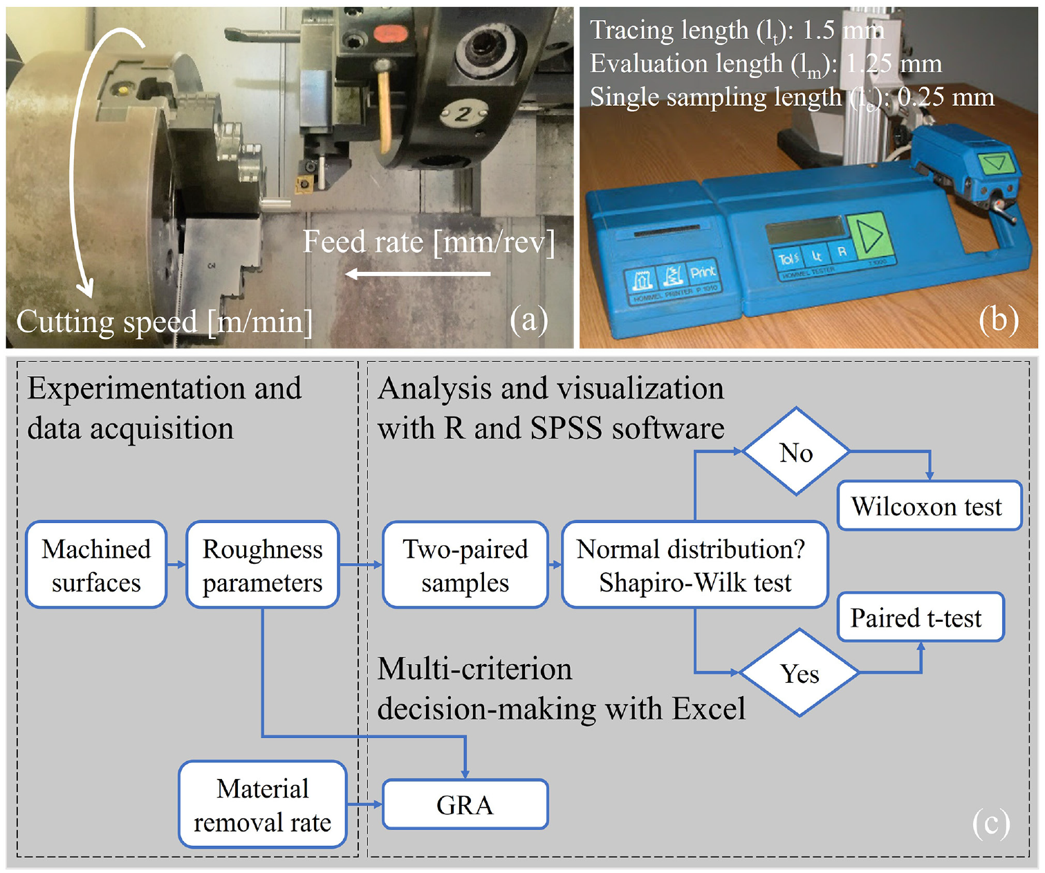
(a) Experimental setup, the white arrows represent the machining process parameters, (b) roughness tester and conditions used to evaluate the machined surfaces and (c) methodology for data treatment and analysis.

Titanium alloys

Ti6Al7Nb and Ti6Al4V alloy billets with a 12 mm diameter were used in the turning experiments. According to TiFast S.r.l., they were produced by vacuum arc remelting, were hot rolled, annealed and cold finished. The as-received alloys had an average surface roughness (R_a) of 0.61 ± 0.09 μm (Ti6Al4V) and 0.52 ± 0.03 μm (TiAl7Nb).

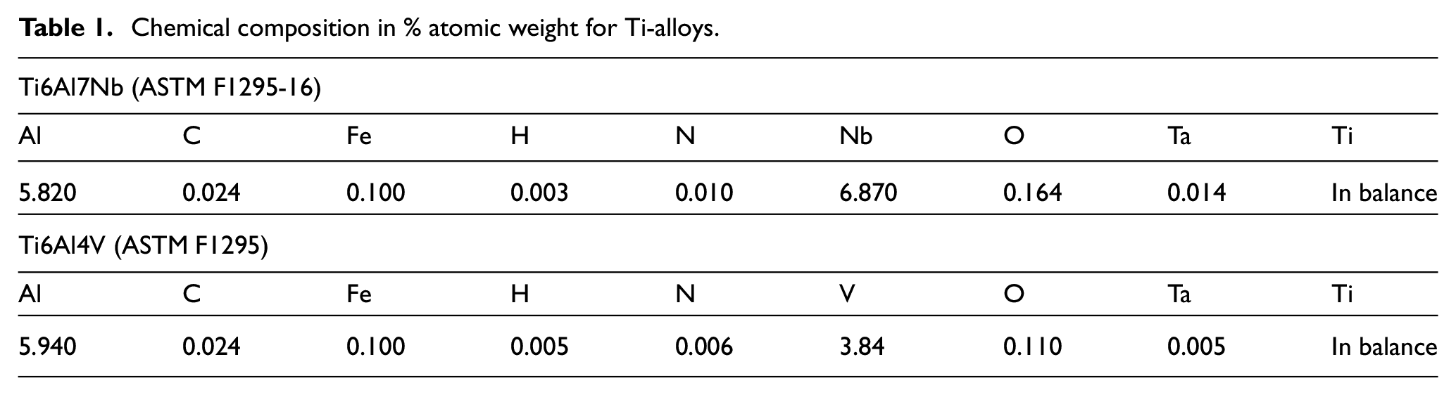
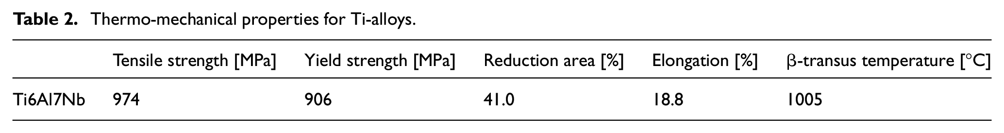
The Ti6Al4V and Ti6Al7Nb alloys presented a microstructure composed of a fine dispersion of α a and β phases. A detailed microstructural report of the alloys is available in a previous publication by the authors.¹³ The Ti-alloys’ chemical composition, as well as thermo-mechanical properties, can be found in Tables 1 and 2, respectively. These values were available in the quality certificate sheets delivered with the alloys.

Table 1.

Chemical composition in % atomic weight for Ti-alloys.

Ti6Al7Nb (ASTM F1295-16)
Al	C	Fe	H	N	Nb	O	Ta	Ti
5.820	0.024	0.100	0.003	0.010	6.870	0.164	0.014	In balance
Ti6Al4V (ASTM F1295)
Al	C	Fe	H	N	V	O	Ta	Ti
5.940	0.024	0.100	0.005	0.006	3.84	0.110	0.005	In balance

Table 2.

Thermo-mechanical properties for Ti-alloys.

	Tensile strength [MPa]	Yield strength [MPa]	Reduction area [%]	Elongation [%]	β-transus temperature [°C]
Ti6Al7Nb	974	906	41.0	18.8	1005

Dry turning experiments

The oblique dry turning tests were conducted on a CNC turning centre Kingsbury MHP 50 with 18 kW power and a maximum revolution speed of 4500 rpm. PVD TiAlN + TiN coated tools with chip breaker, designation CNMG 120408-MF1 TS2000 (from Seco tools), were employed in a tool holder model C3-PCLNL-22040-12 (from Sandvik Coromant). The insert geometry was suitable for machining stainless steels, super alloys and titanium alloys in semi-finishing and finishing operations.

The cutting parameters were chosen following: (1) the manufacturer’s recommendations (a_p: 0.25–3.0 mm, f: 0.08–0.3 mm/rev; v_c: 50–70 m/min); (2) the type of operation (finishing), which is why a low feed rate (0.05, 0.1 and 0.15 mm/rev) and depth-of-cut (0.5 mm) were applied; (3) the research goals, which were, minimize the surface roughness, without compromising the productivity, by controlling the feed rate and cutting speed; (4) the state-of-the-art, including a review on cutting parameters for machining titanium alloys by Festas et al.⁴¹ and the optimization work done by Mazid et al.⁴² These authors carried out turning tests in a Ti6Al4V alloy, and although they applied cutting fluid, they observed that for a cutting configuration similar to ours, the conditions that minimized the surface roughness (R_a: 0.8 μm) were an a_p of 0.5 mm, an f of 0.1 mm/rev and a v_c of 50 m/min.

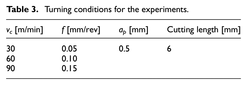
As displayed in Table 3, a factorial design (Taguchi L9 orthogonal array) with three levels of cutting speed (v_c) and feed rate (f) was implemented for the turning experiments. A total of nine machining conditions were investigated. The tests were repeated twice to stabilize the sample mean and standard deviation and increase the statistical inference reliability.⁴³

Table 3.

Turning conditions for the experiments.

v_c [m/min]	f [mm/rev]	a_p [mm]	Cutting length [mm]
30	0.05	0.5	6
60	0.10
90	0.15

The CNMG inserts selected for the machining tests had eight cutting edges. Three cutting edges were used per insert, as each one completed the tests and repetitions done under the same feed rate (f). The maximum working time per cutting edge was below 1.5 min, corresponding to the tests carried out when f was 0.05 mm/rev. For this cutting time, as expected, there were no modifications to the tools. Indeed, the cutting edges were observed periodically, with an optical microscope to guarantee that. Besides, the cutting length was short to prevent tool wear from influencing the individual responses of each roughness parameter since the alloys could present different wear behaviours.

Surface roughness measurements

The surface finish was evaluated with a roughness metre Model T1000 with LV15 diamond probe, both from the Hommelwerke™ company, as shown in Figure 1(b). The mechanical stylus probe acquired the surface roughness profile along 1.5 mm, the defined tracing length (l_t), as presented in Figure 2 After that, several roughness parameters that describe the surface finish were estimated.

Figure 2.

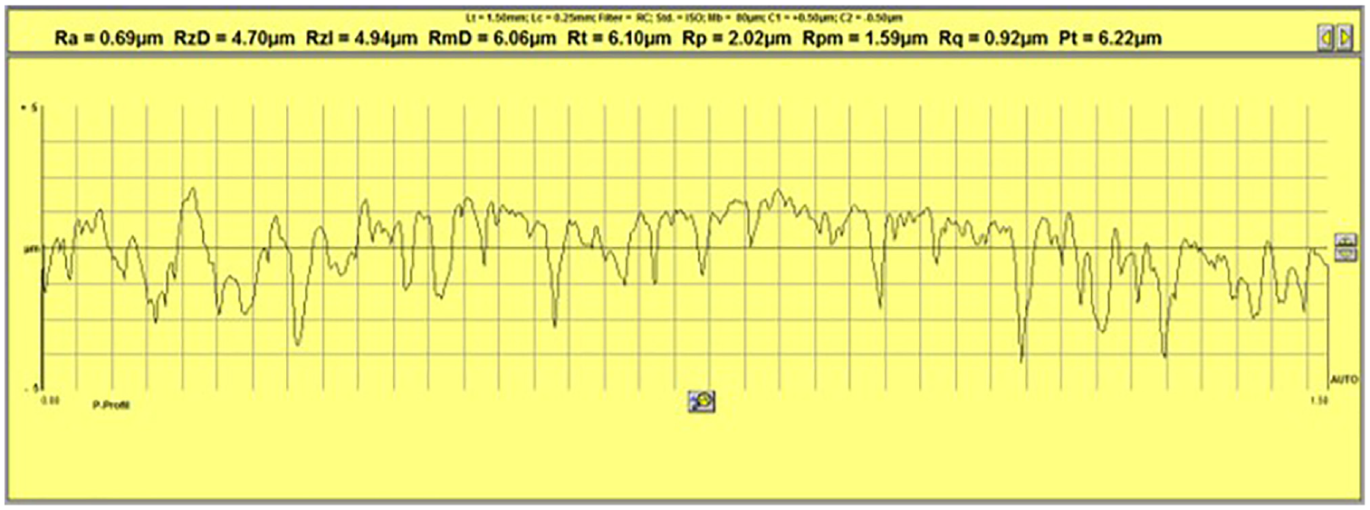
Primary profile for the as-received Ti6Al4V alloy and roughness parameters.

The parameters selected for this work, and their description, can be found in Figure 3. For every roughness parameter, four measurements were taken, two per specimen, spaced approximately at 180°, making a total of 36 observations collected for each alloy.

Figure 3.

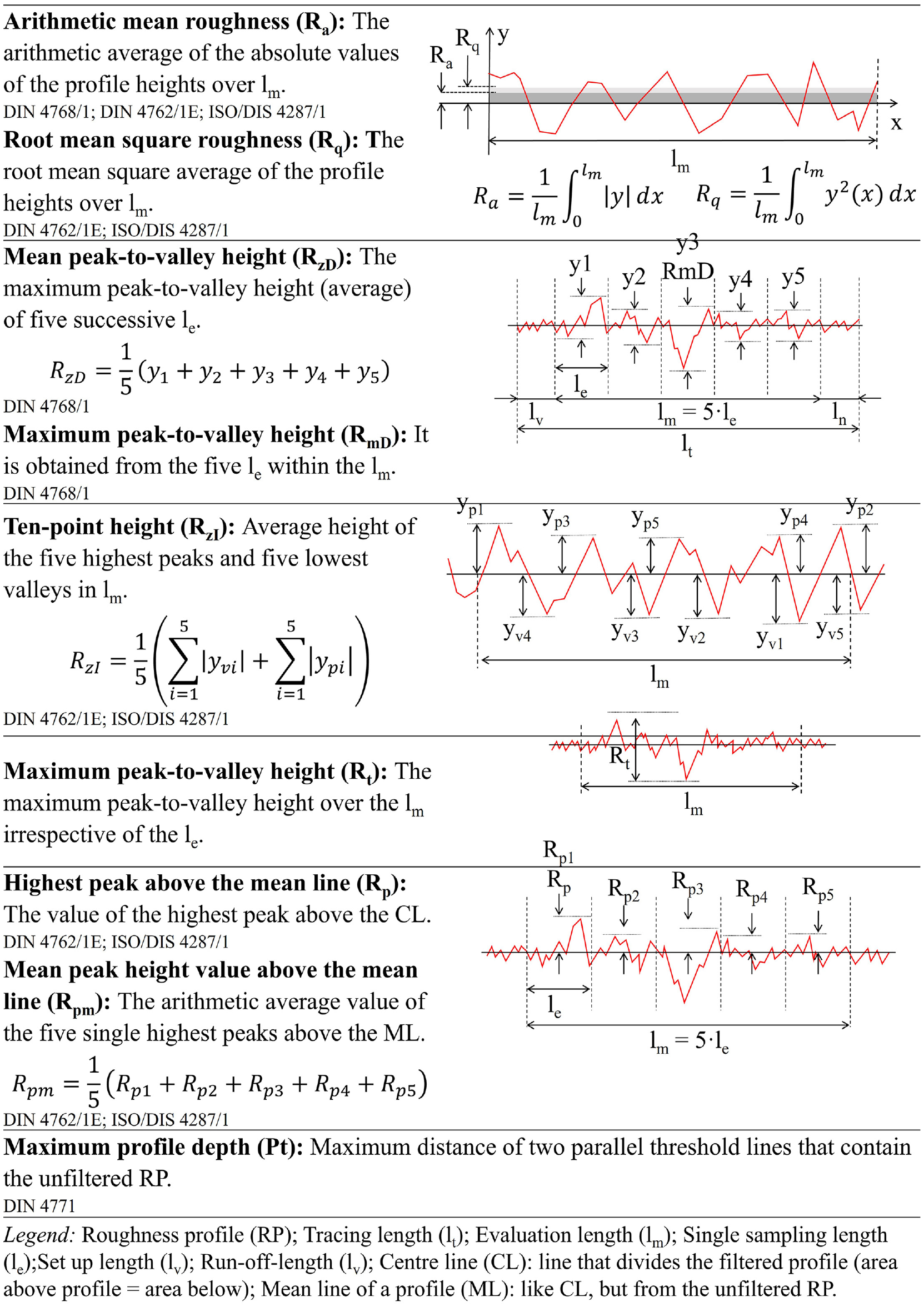
Description of the roughness parameters analysed in the scope of this work. (Hommelwerk cortesy: Hommel Tester T1000 manual).

Data treatment

As shown in Figure 1(c), after the roughness measurements, the dataset was uploaded to R ×64 4.0.3 and IBM SPSS Statistics 27 for further analysis. As mentioned before, one of the goals of this work was to determine if there was a significant difference between the surface finish of two titanium alloys machined under the same cutting conditions. Therefore, paired hypothesis t-test was used to compare the corresponding expected mean values of each surface roughness parameter of two related groups (alloys).

Hypothesis testing consisted of (1) formulating the null (H₀) and alternative hypothesis (H_a), as well as the significance level (α). (2) Select the appropriate test and state the relevant test statistic. (3) Determine the value of the test statistic and the p-value. (4) Compare the p-value with the significance level. Then, if p-value≤α, H₀ is rejected. Otherwise, if p-value >α, H₀ cannot be rejected.⁴⁴

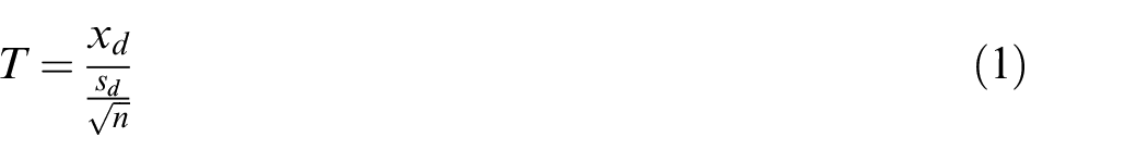
For the paired t-test, the null hypothesis (H₀) was that the two means (alloys) were equal, which was the same as saying that the population mean difference was zero. As demonstrated in equation (1), to determine the test statistic (T), three fundamental data values were required, namely the average of the differences between the paired data (x_d), the standard deviation for the paired difference (s_d) and the number of paired differences (n). Afterwards, the estimated test statistic was compared with the tabulated, taken from the known probability distribution (t-distribution). Moreover, the test statistic was utilized for calculating the p-value. In practice, all these steps were performed by statistical software.

T = \frac{x_{d}}{\frac{s_{d}}{\sqrt{n}}}

(1)

As shown in Figure 1(c), the paired t-test was used when the paired differences followed a normal distribution. Due to the sample size (36 observations), the paired difference normality was checked with a Shapiro-Wilk test.⁴⁵ This test assumes a null hypothesis (H₀) where the sample, in our case paired difference, comes from a normally distributed population.

When the normality was rejected, the non-parametric Wilcoxon signed-rank test was used to determine if the two paired groups (two alloys machined under the same conditions) were different from one another in a statistically significant manner. The test statistic was determined by (1) calculating the absolute difference between groups. (2) Determining the rank of the absolute difference between the groups. If the absolute difference is zero, exclude the pair. (3) Computing de positive and negative rankings. The Wilcoxon test statistic is the sum of the positive rankings. Once again, all these steps were performed by statistical software.

The statistical inference was followed by multi-objective optimization with Grey relational analysis (GRA). Ten responses, including nine surface roughness parameters (R_a, R_q, R_mD, R_zD, R_zI, R_t, R_pm, R_p) and the maximum material removal rate (MMR), were included in the GRA. MMR was included to consider the process productivity, that is the volume of material removed per minute and was estimated by the multiplication of the cutting speed (v_c), feed rate (f) and depth-of-cut (a_p) as indicated in Sadeghifar et al.⁴⁶ The goal was to find optimal machining conditions for both alloys.

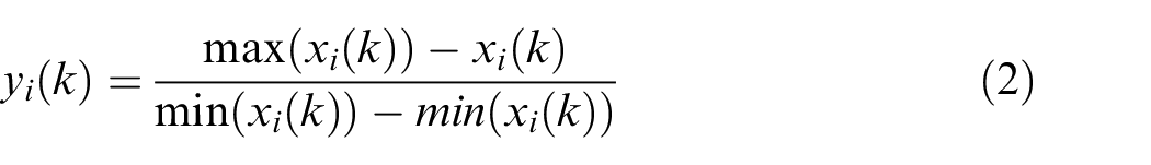
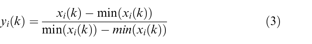
GRA implementation began with dataset normalization. At this step, the original raw responses (x_i (k)), which had their specific scales, were converted into comparable data, ranging from 0 to 1 (y_i (k)). Normalization was done using two equations, one for the ‘smaller-the-better’ responses (equation (2)), that is the nine roughness parameters and the other (equation (3)) for the ‘greater-the-better’ attribute, in this case, the MMR.

y_{i} (k) = \frac{max (x_{i} (k)) - x_{i} (k)}{min (x_{i} (k)) - \min (x_{i} (k))}

(2)

y_{i} (k) = \frac{x_{i} (k) - min (x_{i} (k))}{min (x_{i} (k)) - \min (x_{i} (k))}

(3)

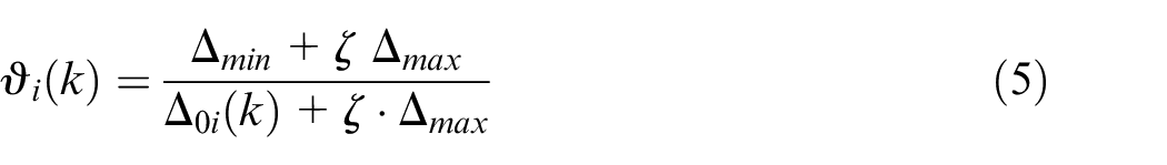
After that, the deduction of the deviation sequence (Δ_oi), as well as the estimation of the Grey relational coefficient (ϑ_i (k)) was carried out using equations (4) and (5). Δ_min and Δ_max correspond to the maximum and minimum from the deviation sequence (Δ_oi). In equation (5), the term ζ is called distinguish factor and was 0.5 suggested by Mia et al.⁴⁷

Δ_{0 i} = | y_{0} (k) - y_{i} (k) |

(4)

ϑ_{i} (k) = \frac{Δ_{\min} + ζ Δ_{\max}}{Δ_{0 i} (k) + ζ \cdot Δ_{\max}}

(5)

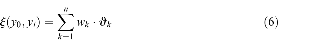
Afterwards, as presented in equation (6), the multi-responses were converted into a single value called Grey relational grade (ξ), which was calculated by combining the Grey relational coefficient (ϑ_k) with a weight value (w_k). In the current study, all the responses had the same weight, as suggested in Mia et al.⁴⁷

ξ (y_{0}, y_{i}) = \sum_{k = 1}^{n} w_{k} \cdot ϑ_{k}

(6)

Finally, the Grey relational order corresponds to the descending order of the Grey relational grades. The optimal run was the one with the highest Grey relational grade, corresponding to rank 1. All these steps were implemented in Microsoft Excel.

Results

This section details the main findings regarding the surface texture attained when turning two biomedical Ti-alloys, starting with the boxplot visualization containing the distribution for the surface roughness parameters for both titanium alloys, as shown in Figure 4. The measurements from surfaces machined with the same feed rate (f) present the same colour, that is yellow (0.05 mm/rev), blue (0.10 mm/rev) and red (0.15 mm/rev), whereas the ones attained at the same level of cutting speed (v_c) present the same shape, namely cross (30 m/min), circle (60 m/min) or triangle (90 m/min).

Figure 4.

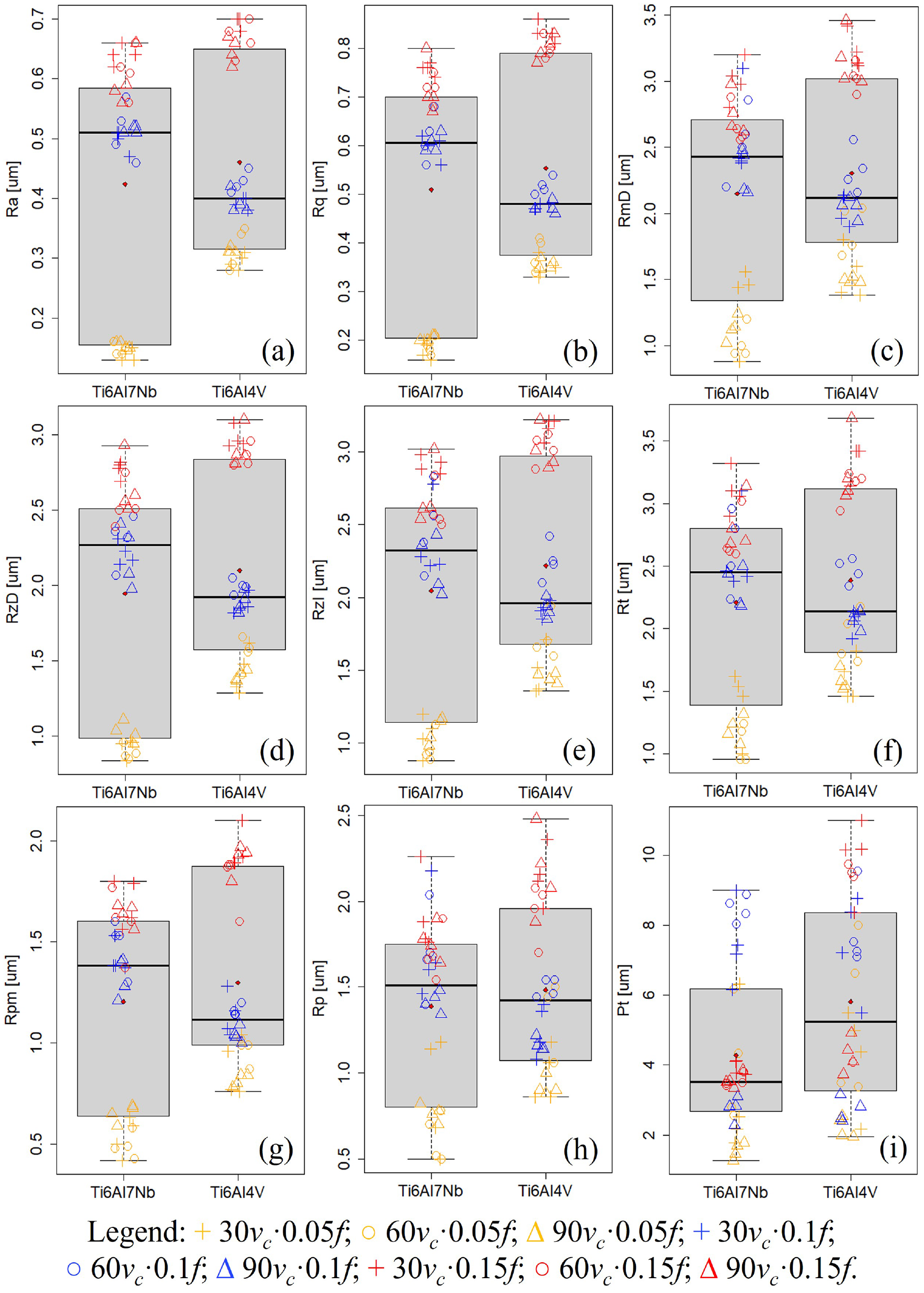
Ti-alloys roughness distribution for R_a (a), R_q (b), R_mD (c), R_zD (d), R_zI (e), R_t (f), R_pm (g), R_p (h) and P_t (i). The black lines represent the distribution median, while the red dot is the mean.

Figure 4 indicates that for several roughness parameters, including R_a (a), R_q (b), R_mD (c), R_zD (d), R_zI (e), R_t (f), R_pm (g) and R_p (h) the measurements are clustered by colour, meaning feed rate. These clusters were separated, as is the case for the Ra (a), Rq (b) and RzD (d) in Ti6Al4V surfaces, while sometimes they were overlaid. The overlaps were slight, as in the R_a (a), R_q (b) and R_zD (d) for Ti6Al7Nb surfaces and R_pm (g) for both alloys, or more evident as observed for R_mD (c), R_zI (e), R_t (f), R_p (h) for both alloys. As expected, the parameters that emphasize the deviations of the roughness profile, namely R_mD (c), R_zI (e) and R_t (f) for the peak-to-valley height, and R_p (h) for the peak height, culminated in distributions with overlaps, due to higher data variability. The corresponding parameters, namely R_zD (d) and R_pm (g), that divide the profile in sampling lengths and look at its average, reduced the data variability, which increased the separation between clusters. The same applies to R_a (a) and R_q (b).

The feed rate effect on the surface roughness of machined surfaces is well reported in the state-of-the-art.^26,48 It is a well-established fact that increasing the feed rate in machining operations leads to rougher surfaces, which is reflected in roughness measurements in Figure 4(a) to (h). The results from Figure 4(a) to (h) also indicate that lower and higher levels of feed rate (0.05 and 0.15 mm/rev) promoted smoother surfaces for Ti6Al7Nb alloy (R_a was 0.15 ± 0.01 and 0.62 ± 0.04 μm) than for Ti6Al4V alloy (R_a was 0.31 ± 0.02 and 0.67 ± 0.03 μm). On the other hand, when the feed rate was 0.1 mm/rev, the Ti6Al4V alloy surfaces were smoother (R_a was 0.40 ± 0.02 μm) compared to Ti6Al7Nb alloy (R_a was 0.51 ± 0.03 μm).

Additionally, the roughness measurements from Figure 4(a) to (h) suggest that regardless of the cutting speed, for Ti6Al7Nb alloy, it is possible to increase the feed rate from medium (0.1 mm/rev) to high (0.15 mm/rev) without compromising (severely) the surface roughness (R_a from 0.51 ± 0.03 to 0.62 ± 0.04 μm). An analogous conclusion was established for Ti6Al4V alloy, as an increase from lower (0.05 mm/rev) to medium (0.1 mm/rev) feed rate does not impact (drastically) the surface roughness (R_a from 0.31 ± 0.02 to 0.40 ± 0.02 μm). This outcome arose from the asymmetries presented by the distributions for the alloys. As shown in Figure 4(a) to (h), for Ti6Al7Nb alloy, the roughness distributions were left-skewed (mean < median), while for Ti6Al4V alloy, the distributions were right-skewed (mean > median), as indicated in Figure 4(a) to (i). The roughness values attained at 0.05 mm/rev for Ti6Al7Nb alloy surfaces (R_a: 0.15 ± 0.01 μm) decreased the distribution mean and enhanced the left skewing.

Furthermore, Figure 4 suggests that the roughness data does not show any specific trend in terms of cutting speed (v_c). A similar indication was given by the data in Table 4, which relates the measurements for each roughness parameter with the cutting conditions. The roughness values from Table 4 were obtained from the average of the four measurements. Table 4 indicates that the average roughness (R_a) for Ti6Al7Nb surfaces varied between 0.14 ± 0.01 and 0.64 ± 0.02 μm and from 0.30 ± 0.01 to 0.70 ± 0.01 μm for Ti6Al4V alloy surfaces, corresponding to a roughness grade number of ranging from N4 to N6.

Table 4.

Roughness response (average and standard deviation) and material removal rate as a function of the cutting conditions.

v_c [m/min]	f [mm/rev]	R_a	R_q	R_mD	R_zD	R_zI	R_t	R_pm	R_p	P_t	MRM [m³/min]
Ti6Al4V
30	0.05	0.30 ± 0.01	0.35 ± 0.02	1.55 ± 0.20	1.43 ± 0.15	1.49 ± 0.16	1.60 ± 0.17	0.88 ± 0.14	0.99 ± 0.16	4.26 ± 1.46	750
	0.1	0.39 ± 0.01	0.48 ± 0.01	2.03 ± 0.12	1.88 ± 0.07	1.92 ± 0.05	2.06 ± 0.10	1.14 ± 0.11	1.26 ± 0.15	7.47 ± 1.47	1500
	0.15	0.70 ± 0.01	0.83 ± 0.02	3.23 ± 0.14	2.98 ± 0.07	3.16 ± 0.07	3.35 ± 0.14	1.95 ± 0.10	2.15 ± 0.16	9.93 ± 1.11	2250
60	0.05	0.32 ± 0.04	0.38 ± 0.03	1.88 ± 0.18	1.56 ± 0.11	1.73 ± 0.15	1.94 ± 0.21	0.97 ± 0.07	1.27 ± 0.24	5.38 ± 2.30	1500
	0.1	0.43 ± 0.02	0.52 ± 0.02	2.33 ± 0.17	2.00 ± 0.05	2.25 ± 0.13	2.47 ± 0.10	1.16 ± 0.03	1.50 ± 0.05	7.86 ± 1.15	3000
	0.15	0.67 ± 0.03	0.80 ± 0.02	3.03 ± 0.11	2.86 ± 0.07	3.02 ± 0.11	3.14 ± 0.14	1.81 ± 0.14	1.95 ± 0.17	8.19 ± 2.74	4500
90	0.05	0.31 ± 0.01	0.36 ± 0.01	1.50 ± 0.02	1.40 ± 0.03	1.45 ± 0.03	1.59 ± 0.08	0.82 ± 0.03	0.92 ± 0.05	2.23 ± 0.29	2250
	0.1	0.39 ± 0.02	0.47 ± 0.01	2.05 ± 0.08	1.89 ± 0.07	1.93 ± 0.07	2.08 ± 0.07	1.04 ± 0.04	1.17 ± 0.04	2.72 ± 0.35	4500
	0.15	0.65 ± 0.02	0.80 ± 0.03	3.17 ± 0.21	2.91 ± 0.13	3.01 ± 0.15	3.26 ± 0.29	1.91 ± 0.08	2.17 ± 0.25	4.30 ± 0.50	6750
Ti6Al7Nb
30	0.05	0.14 ± 0.01	0.18 ± 0.02	1.34 ± 0.31	0.93 ± 0.06	1.05 ± 0.13	1.41 ± 0.28	0.54 ± 0.09	0.88 ± 0.34	3.20 ± 2.10	750
	0.1	0.50 ± 0.02	0.60 ± 0.03	2.58 ± 0.35	2.21 ± 0.08	2.38 ± 0.27	2.59 ± 0.34	1.42 ± 0.08	1.72 ± 0.32	7.44 ± 1.17	1500
	0.15	0.64 ± 0.02	0.76 ± 0.01	3.01 ± 0.17	2.77 ± 0.06	2.91 ± 0.06	3.10 ± 0.17	1.69 ± 0.12	1.92 ± 0.23	3.94 ± 0.20	2250
60	0.05	0.15 ± 0.01	0.19 ± 0.02	1.02 ± 0.12	0.89 ± 0.05	0.97 ± 0.11	1.09 ± 0.15	0.50 ± 0.06	0.63 ± 0.14	3.97 ± 1.67	1500
	0.1	0.51 ± 0.05	0.62 ± 0.05	2.54 ± 0.27	2.30 ± 0.17	2.48 ± 0.29	2.63 ± 0.32	1.49 ± 0.13	1.70 ± 0.26	8.48 ± 0.37	3000
	0.15	0.61 ± 0.04	0.72 ± 0.03	2.67 ± 0.15	2.54 ± 0.15	2.61 ± 0.15	2.72 ± 0.20	1.59 ± 0.17	1.70 ± 0.15	3.56 ± 0.18	4500
90	0.05	0.16 ± 0.01	0.21 ± 0.01	1.13 ± 0.09	1.03 ± 0.07	1.09 ± 0.09	1.20 ± 0.10	0.65 ± 0.05	0.77 ± 0.05	1.56 ± 0.23	2250
	0.1	0.52 ± 0.01	0.61 ± 0.02	2.32 ± 0.17	2.20 ± 0.20	2.23 ± 0.20	2.33 ± 0.16	1.33 ± 0.10	1.42 ± 0.06	2.76 ± 0.34	4500
	0.15	0.60 ± 0.04	0.72 ± 0.06	2.76 ± 0.16	2.65 ± 0.19	2.70 ± 0.22	2.83 ± 0.21	1.64 ± 0.05	1.77 ± 0.11	3.57 ± 0.22	6750

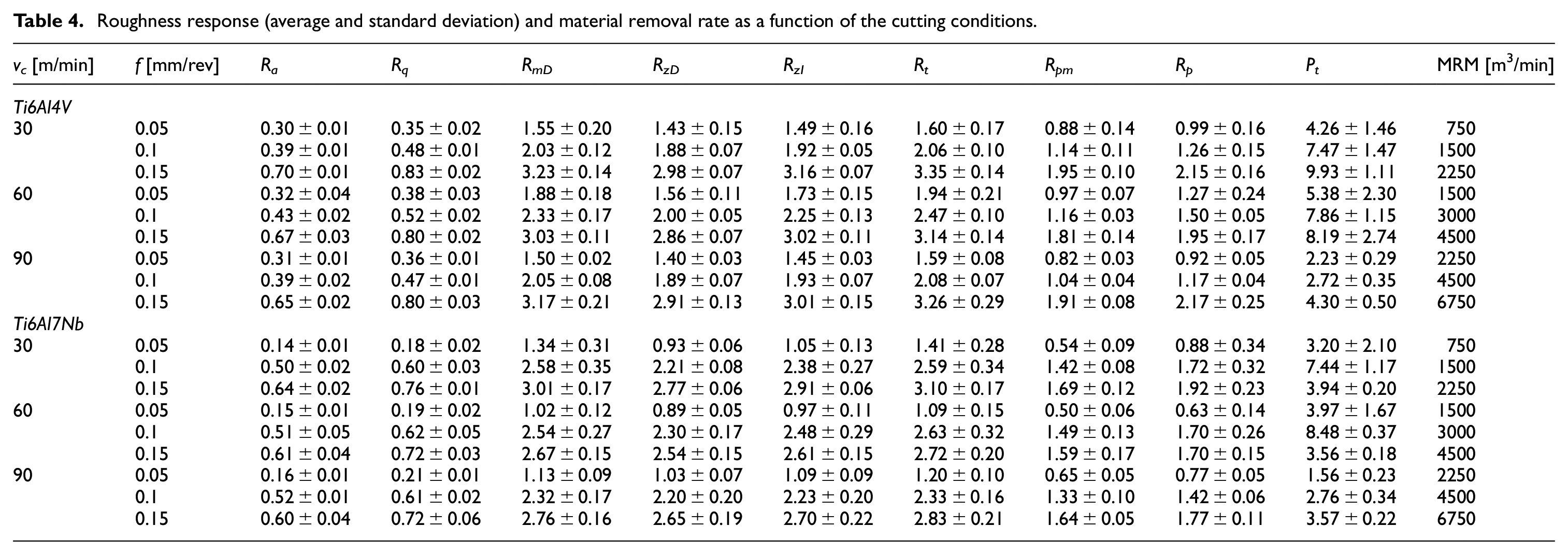
In Table 4, it was observed that, when assessing the distance between peaks and valleys, R_t > R_mD > R_zI > R_zD for all the tested conditions. As expected, the parameters that resulted from the evaluation of the tracing length (R_t and R_mD) were higher than the parameters that counted for the average of the sample sizes (R_zI and R_zD). R_t was the highest value since it detects the higher peak and the lowest valley in the tracing length, followed by R_mD, which detects the same thing, but within the sample sizes. A comparable conclusion was established for the average parameters R_zI (tracing length) and R_zD (sample sizes).

Among the roughness parameters, the maximum profile depth (P_t), shown in Figure 4(i), presents a random distribution, perhaps because this parameter was calculated from the unfiltered roughness profile and is the most sensitive to profile changes.

Statistical inference

Normality test

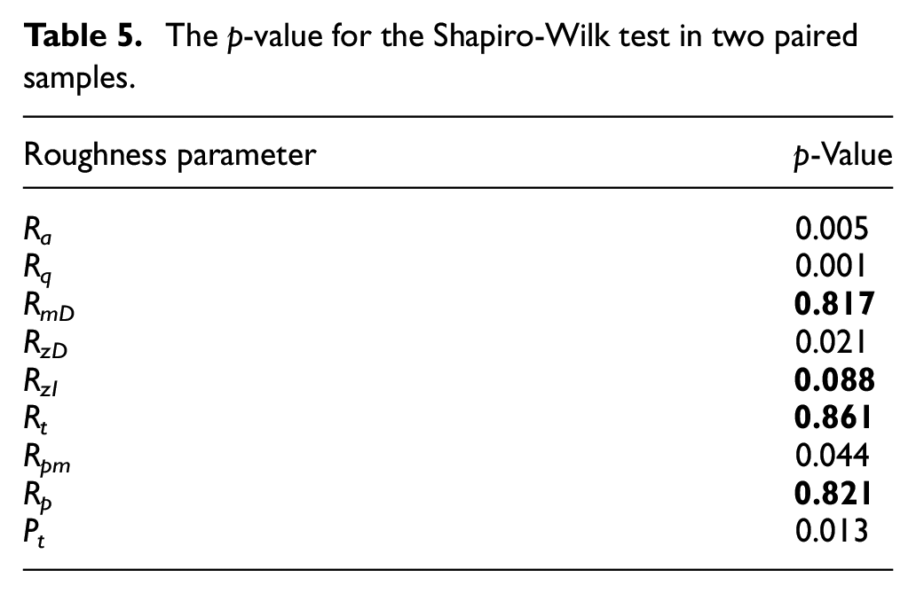
The Shapiro-Wilk test was used to check the normality of the paired differences associated with each dependent variable (R_a, R_q, R_mD, R_zD, R_zI, R_t, R_pm, R_p, P_t). In the scope of the conducted work, the null hypothesis ‘H₀: The dependent variable paired differences follow a normal distribution in the population of Ti-alloys surfaces’ cannot be rejected if the p-value >0.05, while if p-value ≤0.05 the null hypothesis is rejected in favour of the alternative hypothesis which is ‘H_a: The dependent variable paired differences does not follow a normal distribution in the population of Ti-alloys surfaces’.

Table 5 shows that the p-value (R_a, R_q, R_zD, R_pm, P_t) ≤0.05 which rejects the null hypothesis H₀ in favour of H_a (at a 5% significance level) and, thus, one cannot assume that R_a, R_q, R_zD, R_pm and P_t followed a normal distribution. For R_mD, R_zI, R_t and R_p, since the p-value >0.05, H₀ cannot be rejected (at a 5% level), so the normality of differences can be assumed (highlighted in bold in Table 5).

Table 5.

The p-value for the Shapiro-Wilk test in two paired samples.

Roughness parameter	p-Value
R_a	0.005
R_q	0.001
R_mD	0.817
R_zD	0.021
R_zI	0.088
R_t	0.861
R_pm	0.044
R_p	0.821
P_t	0.013

The histogram of differences, and the Q-Q plots, were visualized to substantiate these findings. Figure 5 shows these graphs for one case where the normality of differences can be assumed (R_p) and for another where it is not (R_a). Figure 5(a) indicates that when the differences follow a normal distribution, the histogram is relatively symmetric about the mean (0.097) and fits a bell shape that has only one peak (mode: 0.36). Figure 5(b) shows a bimodal distribution (mode: −0.13, 016), which usually indicates that the distribution in the population is not normal. Besides, in normal distributions, the points in the Q-Q plot define a line, as demonstrated in Figure 5(c).

Figure 5.

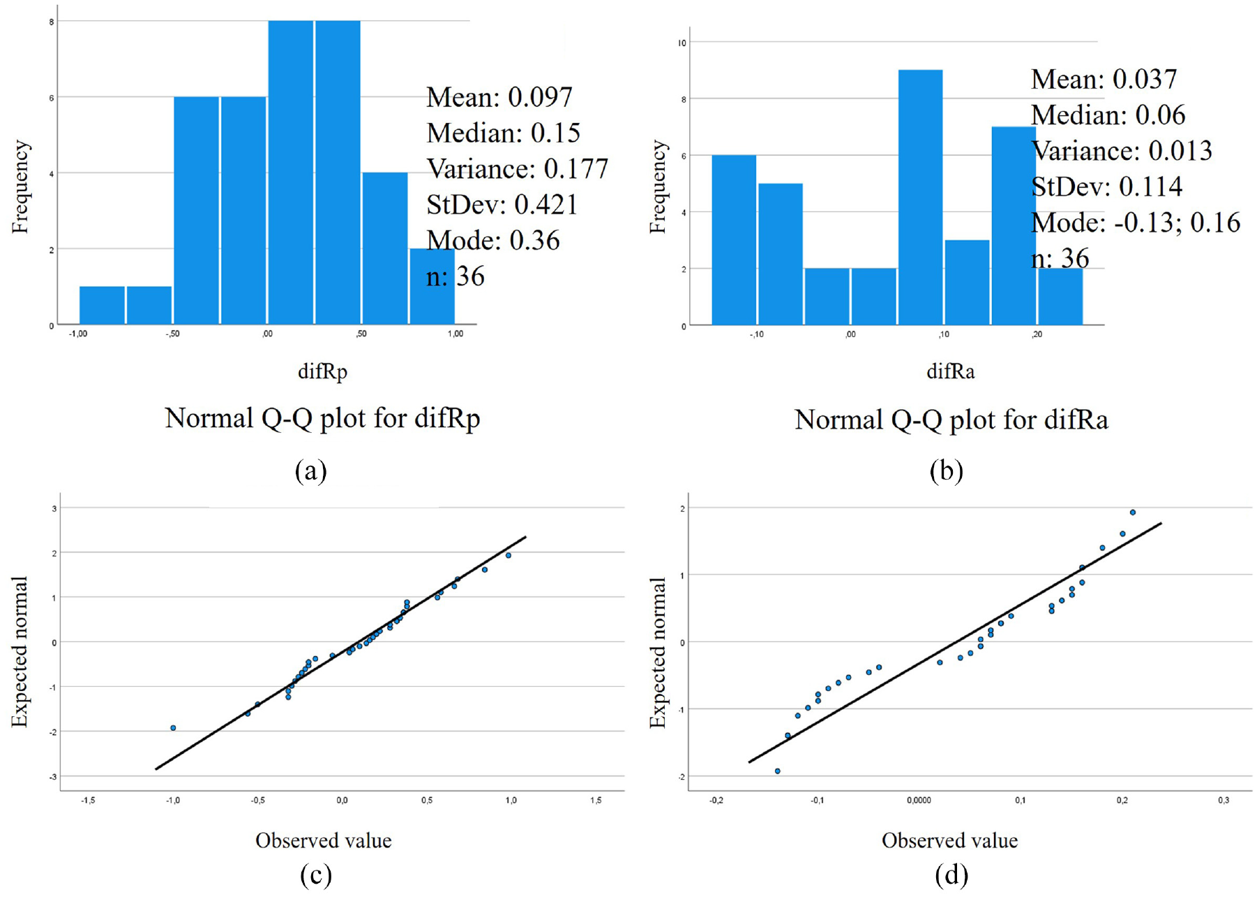
Histogram of differences with descriptive statistics for Rp (a) and Ra (b). Q-Q plot for Rp (c) and Ra (d).

Paired t-test

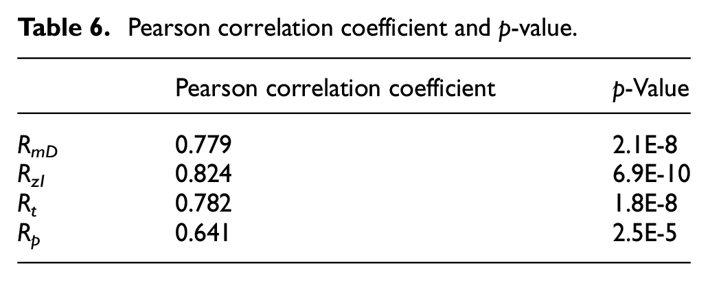
Since one assumption to performing paired t-test is to assure that the two samples are strongly related to being paired, the Pearson correlation coefficient was calculated. Table 6 shows that there was statistical evidence to support that the two samples can be paired as the null hypothesis, ‘H₀: The Pearson correlation coefficient is equal to zero, therefore a linear relationship between the paired items does not exist’ was rejected (p-value (R_mD, R_zI, R_t, R_p)≤0.05) in favour of the alternative hypothesis, ‘H_a: The Pearson correlation coefficient is different from zero, therefore a linear relationship between the paired items exists’ at a 5% significance level. The high Pearson correlation coefficient (Table 6) also implies a strong relationship between the paired samples.

Table 6.

Pearson correlation coefficient and p-value.

	Pearson correlation coefficient	p-Value
R_mD	0.779	2.1E-8
R_zI	0.824	6.9E-10
R_t	0.782	1.8E-8
R_p	0.641	2.5E-5

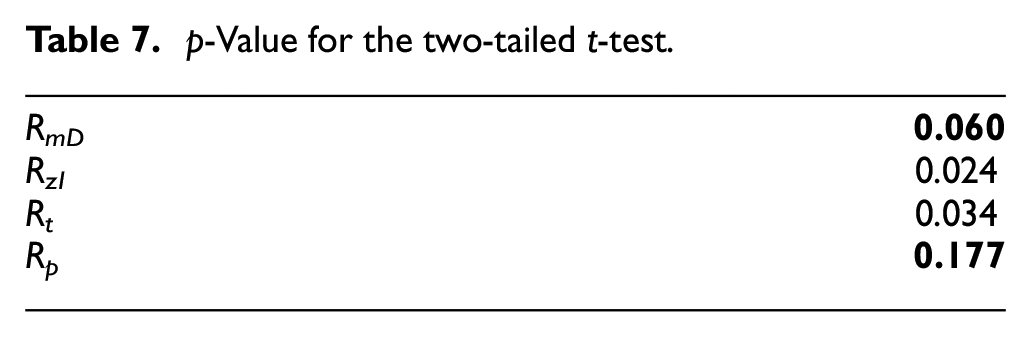
For the variables that presented a normal distribution of the differences (highlighted in bold in Table 5) as well as a strong Pearson correlation coefficient (Table 6), t-testing was performed to check if ‘there was any significant difference in the surface roughness of Ti-alloys surfaces machined under the same cutting conditions (H₀)?’. The Table 7 results indicate that the null hypothesis H₀ was rejected for R_zI and R_t, so it was possible to conclude that for these parameters the mean surface roughness of machined Ti6Al4V and Ti6Al7Nb alloy surfaces were statistically different. While for R_mD and R_p the null hypothesis H₀ cannot be rejected and consequently there are no significant differences between the mean surface roughness of Ti6Al4V and Ti6Al7Nb alloy surfaces (highlighted in bold in Table 7).

Table 7.

p-Value for the two-tailed t-test.

R_mD	0.060
R_zI	0.024
R_t	0.034
R_p	0.177

Wilcoxon test

For the variables that do not follow a normal distribution of the differences (Table 5), the Wilcoxon test was performed to check if there was any significant difference in the surface roughness of Ti-alloys machined under the same conditions (H₀)? Accordingly, to Table 8 this hypothesis was rejected for R_q, R_zD and P_t as the p-value ≤0.05 at a 5% significance level, which means that the median roughness when changing the material to be machined from Ti6Al4V to Ti6Al7Nb alloy was statistically different. For R_a and R_pm, the null hypothesis H₀ cannot be rejected as the p-value >0.05 at a 5% significance level (highlighted in bold in Table 8), meaning that the median roughness when changing the Ti-alloy did not present significant differences.

Table 8.

p-Value for the paired Wilcoxon test.

Roughness parameter	p-Value
R_a	0.067
R_q	0.044
R_zD	0.038
R_pm	0.104
P_t	0.003

Multi-objective optimization

Table 9 presents the Grey relational order achieved for both alloys. In Appendix A, the results from the intermediate steps, namely normalization (Table A1), deviation sequence (Table A2) and Grey relational grade (Table A3), which led to this ranking can be found.

Table 9.

Grey relational grade and rank.

	f [mm/rev]	v_c [m/min]	Ti6Al4V		Ti6Al7Nb
	f [mm/rev]	v_c [m/min]	Grey relational grade	Rank	Grey relational grade	Rank
1	0.05	30	0.863	2º	0.807	3º
2	0.05	60	0.715	3º	0.889	1º
3	0.05	90	0.929	1º	0.844	2º
4	0.1	30	0.595	5º	0.390	8º
5	0.1	60	0.528	6º	0.391	7º
6	0.1	90	0.674	4º	0.472	4º
7	0.15	30	0.340	9º	0.366	9º
8	0.15	60	0.383	8º	0.412	6º
9	0.15	90	0.442	7º	0.448	5º

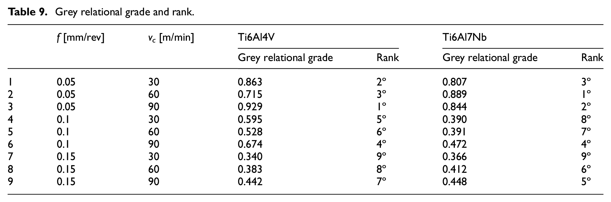
The optimal run was the one with a higher Grey relational grade, which was attained at a low feed rate (0.05 mm/rev) for both alloys. However, at a high cutting speed (90 m/min) for Ti6Al4V and medium cutting speed (60 m/min) for Ti6Al7Nb alloy. Nevertheless, for the Ti6Al7Nb alloy, the rank second position was at 90 m/min. Therefore, it seems reasonable to machine both alloys at the same cutting speed (90 m/min), if needed, to improve the process productivity without neglecting the surface texture. The worst conditions for machining Ti6Al4V alloy (rank 7, 8 and 9) were at a high feed rate (0.15 mm/rev) for all the cutting speeds, while for Ti6Al7Nb alloy, they were at a low cutting speed (30 m/min) combined with medium (0.10 mm/rev) and high (0.15 mm/rev) feed rate (rank 8 and 9).

Furthermore, Table 9 indicates that for Ti6Al4V alloy, the ranking was clustered by feed rate, meaning that the positions 1–3, 4–6 and 6–9 correspond to the conditions with low (0.05 mm/rev), medium (0.1 mm/rev) and high (0.15 mm/rev) feed rate. This was not observed for the medium (0.1 mm/rev) and high (0.15 mm/rev) feed rates for the Ti6Al7Nb alloy. Besides, these results agree with the boxplots from Figure 4, where it was observed that for Ti6Al4V alloy, the transitions between clusters with the same feed rate were well separated, while for Ti6Al7Nb alloy the clusters corresponding to medium (0.1 mm/rev) and high (0.15 mm/rev) levels of feed rate were overlaid for many roughness parameters.

Discussion

As point-out previously, the main goal of this research was to answer the following questions: Do the alloys behave similarly, in terms of surface finish, when machined under the same conditions? Will this depend on the roughness parameter chosen to make the assessment? Which cutting conditions provide a better surface finish for the Ti-alloys? Are they similar?

Statistical inference showed that for some parameters, the mean (R_zI, R_t) and median (R_q, R_zD, P_t) surface roughness was statistically different when changing the alloy, while for others, there was no significant difference in terms of mean (R_mD, R_p) and median (R_a, R_pm). Therefore, the alloys behave similarly for some roughness parameters (R_a, R_mD, R_pm, R_p) and differently for others (R_q, R_zD, R_zI, R_t, P_t). The R_a result was consistent with the findings from Mello et al.,¹¹ as they concluded, through paired t-test, that Ti6Al7Nb and Ti6Al4V alloys presented a similar roughness.

Furthermore, in a different but comparable scope, Folwaczny et al.³¹ reported a significant (for R_p and R_t) and not significant (for R_a, R_zD) increase in the surface roughness of implants after probing. These findings highlight how relevant it is to use several roughness parameters that present different sensitives to the features of the roughness profile (peaks, valleys, height) for defining the surface state, especially when developing standards or quality control procedures. Moreover, it emphasizes the need for observing the data instead of making empirical decisions.

The multi-objective optimization with GRA showed that the optimal conditions that minimize the surface roughness and maximize the material removal rate were attained at 0.05 mm/rev for both alloys. However, at 90 m/min for Ti6Al4V and 60 m/min for Ti6Al7Nb alloy. Moreover, for Ti6Al7Nb alloy, the rank second position was at 0.05 mm/rev and 90 m/min. Therefore, the recommended cutting conditions can be the same. To some extent, these outcomes agree with the findings from other authors, as the optimal conditions for improving the surface finish¹¹ and the specific cutting energy¹² when machining Ti6Al4V and Ti6AL7Nb were the same.

Nonetheless, the Ti6Al4V alloy ranking is clustered by feed rate, while for Ti6Al7Nb alloy is not. These results were consistent with the boxplot visualization from Figure 4. As for Ti6Al4V distribution, the transitions between clusters were defined, while for Ti6Al7Nb, they were overlaid. Therefore, while the optimal conditions were comparable, the overall behaviour was not. Consequently, deducting that the machinability of the alloy is similarly based only on the optimal machining conditions can lead to a precipitous conclusion.

Conclusion

In this work, the surface roughness of two α + β biomedical titanium alloys turned under dry conditions was compared. The effects of the cutting speed (v_c) and feed rate (f), on the surface roughness, were inspected. Several amplitude roughness parameters, including R_a, R_q, R_mD, R_zD, R_zI, R_t, R_pm, R_p and P_t were measured with a stylus probe. Hypothesis testing was used to evaluate the equality of the expected values and population median. Multi-objective optimization was conducted for defining suitable cutting regimes. Some meaningful conclusions can be taken from this work:

The boxplot charts were quite helpful to understand the impact of the cutting conditions on the surface roughness parameters. It seems that the roughness data does not present any specific trend in terms of cutting speed, however the same cannot be said about the feed rate, since as it increases rougher surfaces were attained.

The boxplot charts indicate that Ti6Al7Nb alloy machined surfaces presented a smoother texture for a lower (0.05 mm/rev) and higher (0.15 mm/rev) level of feed rate when compared with Ti6Al4V alloy surfaces, yet at the intermediate level (0.10 mm/rev), this behaviour changes as Ti6Al4V alloy surfaces were smoother.

The results from the hypothesis testing highlight the importance of using several roughness parameters to understand the Ti-alloy surface state because different conclusions, present a comparable finish (R_a, R_mD, R_pm, R_p) or not (R_q, R_zD, R_zI, R_t, P_t), can be drawn depending on the analysed roughness descriptor.

The multi-objective optimization showed that the conditions that improve the surface integrity, without neglecting the process productivity were a low feed rate (0.05 mm/rev) combined with a high cutting speed (90 m/min) for Ti6Al4V alloy and a low feed rate (0.05 mm/rev) combined with a medium cutting speed (60 m/min) for Ti6Al7Nb alloy.

Footnotes

Appendix A

This section contains the results from the intermediate steps, namely data normalization (Table A1), deduction of the deviation sequence (Table A2) and determination of the grey relational grade (Table A3) behind the application of the multi-objective optimization algorithm, that is grey relational analysis. These steps were carried out considering the original data from Table 4.

Acknowledgements

The authors also acknowledge TiFast S.R.L., from Italy, for providing the Ti-alloy.

Declaration of conflicting interests

The author(s) declared no potential conflicts of interest with respect to the research, authorship, and/or publication of this article.

Funding

The author(s) disclosed receipt of the following financial support for the research, authorship, and/or publication of this article: The authors acknowledge the Portuguese Foundation for Science and Technology (FCT) for the PhD grant ref. SFRH/BD/07040/2021.

ORCID iDs

Sílvia Ribeiro Carvalho

Ana Horovistiz

JP Davim

References

Peters

Leyens

. Titanium and titanium alloys fundamentals and applications. Weinheim: Wiley-VCH, 2003.

Costa

Tokuhara

Rocha

, et al. Vanadium ionic species from degradation of Ti-6Al-4V metallic implants: in vitro cytotoxicity and speciation evaluation. Mater Sci Eng C 2019; 96: 730–739.

Gupta

Laubscher

. Sustainable machining of titanium alloys: a critical review. Proc IMechE, Part B: J Engineering Manufacture 2017; 231: 2543–2560.

Sun

Huang

Puleo

, et al. Improved surface integrity from cryogenic machining of Ti-6Al-7Nb alloy for biomedical applications. Procedia CIRP 2016; 45: 63–66.

Lauro

Ribeiro Filho

SLM

Brandão

, et al. Analysis of behaviour biocompatible titanium alloy (Ti-6Al-7Nb) in the micro-cutting. Measurement 2016; 93: 529–540.

Lauro

Brandão

Filho

SLMR

, et al. Behaviour of a biocompatible titanium alloy during orthogonal micro-cutting employing green machining techniques. Int J Adv Manuf Technol 2018; 98: 1573–1589.

Fellah

Labaïz

Assala

, et al. Tribological behavior of Ti-6Al-4V and Ti-6Al-7Nb alloys for total hip prosthesis. Adv Tribol 2014; 2014: 1–13.

Almeida

Horovistiz

Davim

. Digital representation of the wear behaviour of Ti-6Al-4V and Ti-6Al-7Nb biomaterial alloys: a fractal analysis of the worn surface. Proc IMechE, Part J: J Engineering Tribology 2023; 237: 1156–1169.

Avinash

Kumar

SPL

. Investigations on corrosion resistance behavior in micro-milling of Ti-6Al-4V and Ti-6Al-7Nb alloy: a comparative study. J Mech Sci Technol 2020; 34: 3757–3765.

10.

Festas

Carvalho

Horovistiz

, et al. Comparative study of titanium alloys machinability used for medical applications. Proc IMechE, Part E: J Process Mechanical Engineering 2022; 236: 1845–1856.

11.

Mello

Pereira

RBD

Lauro

, et al. Comparison between the machinability of different titanium alloys (Ti–6Al–4V and Ti–6Al–7Nb) employing the multi-objective optimization. J Braz Soc Mech Sci Eng 2021; 43: 1–14.

12.

Filho

SLMR

Pereira

RBD

Lauro

, et al. Investigation and modelling of the cutting forces in turning process of the Ti-6Al-4V and Ti-6Al-7Nb titanium alloys. Int J Adv Manuf Technol 2019; 101: 2191–2203.

13.

Carvalho

Horovistiz

Davim

. Surface topography in machining Ti alloys for biomedical applications: correlative microscopy approach for qualitative and quantitative analysis. Int J Adv Manuf Technol 2021; 114: 683–694.

14.

Yan

Rong

Wang

. The effect of cutting fluids applied in metal cutting process. Proc IMechE, Part B: J Engineering Manufacture 2016; 230: 19–37.

15.

Chomienne

Valiorgue

Rech

, et al. Development of a surface engineering strategy to quantify the sensitivity of surface integrity features in fatigue performance. Proc IMechE, Part B: J Engineering Manufacture 2023; 237: 561–572.

16.

Nicolas-Silvente

Velasco-Ortega

Ortiz-Garcia

, et al. Influence of the titanium implant surface treatment on the surface roughness and chemical composition. Materials 2020; 13: 314.

17.

Alla

Ginjupalli

Upadhya

, et al. Surface roughness of implants: a review. Trends Biomater Artif Organs 2011; 25: 112–118.

18.

Jordana

Susbielles

Colat-Parros

. Periimplantitis and implant body roughness: a systematic review of literature. Implant Dent 2018; 27: 672–681.

19.

Cubillos

dos Santos

Pizzolatti

ALA

, et al. Surface finish of total hip arthroplasty implants: are we evaluating and manufacturing them appropriately? J Test Eval 2021; 49: 4550–4559.

20.

Zein

. Investigation of surface texture and surface residual stresses in the dry face turning process of AL2024-T351. Int J Mech Mechatronics Eng 2020; 20: 123–143.

21.

Chakravarthy

VVK

Rajmohan

Vijayan

, et al. Sustainable drilling of Nano SiC reinforced Al matrix composites using MQL and cryogenic cooling for achieving the better surface integrity. Silicon 2022; 14: 1787–1805.

22.

Ibrahim

Haron

CHC

Ghani

. Surface integrity of Ti-6Al-4V ELI when machined using coated carbide tools under dry cutting condition. Int J Mech Mater Eng 2009; 4: 191–196.

23.

Gadelmawla

Koura

Maksoud

TMA

, et al. Roughness parameters. J Mater Process Technol 2002; 123: 133–145.

24.

Charles

Elkaseer

Thijs

, et al. Effect of process parameters on the generated surface roughness of down-facing surfaces in selective laser melting. Appl Sci 2019; 9: 1256.

25.

Lee

Rasoolian

Silva

, et al. Surface roughness parameter and modeling for fatigue behavior of additive manufactured parts: a non-destructive data-driven approach. Addit. Manuf 2021; 46: 102094.

26.

Çelik

Kilickap

Güney

. Investigation of cutting parameters affecting on tool wear and surface roughness in dry turning of Ti-6Al-4V using CVD and PVD coated tools. J Braz Soc Mech Sci Eng 2017; 39: 2085–2093.

27.

Kamguem

Tahan

Songmene

. Evaluation of machined part surface roughness using image texture gradient factor. Int J Precis Eng Manuf 2013; 14: 183–190.

28.

Berzosa

Rubio

de Agustina

, et al. Geometric optimization of drills used to repair holes in magnesium aeronautical components. Metals 2020; 10: 1534.

29.

ECT

Dumont

Martins

, et al. Investigation of the effects of skewness R_sk and kurtosis R_ku on tribological behavior in a pin-on-disc test of surfaces machined by conventional milling and turning processes. Mater Res 2021; 24: e20200435.

30.

Festas

Pereira

Ramos

, et al. A study of the effect of conventional drilling and helical milling in surface quality in titanium Ti-6Al-4V and Ti-6AL-7nb Alloys for medical applications. Arab J Sci Eng 2021; 46: 2361–2369.

31.

Folwaczny

Rudolf

Frasheri

, et al. Ultrastructural changes of smooth and rough titanium implant surfaces induced by metal and plastic periodontal probes. Clin Oral Investig 2021; 25: 105–114.

32.

Kanlayasiri

Jattakul

Mookam

. Machinability of tool steels machined by electric-discharge machining. SNRU J Sci Technol 2021; 14: 25–31.

33.

Malladi

Saravanan

Gnanavel

, et al. Taguchi based parameter optimization for cutting force reduction in SAE 1045 steel machining with nanofluid. Mater Today Proc 2022; 62: 1325–1329.

34.

Kovalčík

Mašek

Malý

, et al. The effect of coatings on cutting force in turning of C45 Steel. Materials 2022; 15: 1–16.

35.

Pawanr

Garg

Routroy

. Prediction of energy consumption of machine tools using multi-gene genetic programming. Mater Today Proc 2022; 58: 135–139.

36.

Diyaley

Chakraborty

. Metaheuristics-based parametric optimization of multi-pass turning process: a comparative analysis. Opsearch 2020; 57: 414–437.

37.

Gupta

Kumar

, et al. Optimization of process parameters during machining of Ti6Al7Nb by grey relational analysis based on Taguchi. J Phys Conf Ser 2019; 1240: 012121.

38.

Sofuoglu

Orak

. A novel hybrid multi criteria decision making model: application to turning operations. Int J Intell Syst Appl Eng 2017; 3: 124–131.

39.

Sofuoğlu

Arapoğlu

Orak

. Multi objective optimization of turning operation using hybrid decision making analysis. ANADOLU Univ J Sci Technol A Appl Sci Eng 2017; 18: 595–610.

40.

. A revised grey relational analysis method for multicriteria group decision-making with expected utility theory for oil spill emergency management. Math Probl Eng 2021; 2021: 1–13.

41.

Festas

Ramos

Davim

. Machining of titanium alloys for medical application - a review. Proc IMechE, Part B: J Engineering Manufacture 2022; 236: 309–318.

42.

Mazid

Hasan

Ahsan

. An investigation on optimum process parameters in terms of surface roughness for turning titanium alloy Ti-6Al-4V using coated carbide. Int J Eng Mater Manuf 2019; 4: 137–145.

43.

Bao

Wang

. The repetition principle in scientific research. Chin J Integr Med 2011; 9: 937–940.

44.

Mello

Peternelli

. Conhecendo o R: uma visão mais que estatística. 1^a. UFV, 2013.

45.

Laureano

RMS

. Testes de Hipóteses com o SPSS - O Meu Manual de Consulta Rápida. 2^a. Sílabo, 2013.

46.

Sadeghifar

Sedaghati

Jomaa

, et al. Finite element analysis and response surface method for robust multi-performance optimization of radial turning of hard 300M steel. Int J Adv Manuf Technol 2018; 94: 2457–2474.

47.

Mia

Gupta

Lozano

, et al. Multi-objective optimization and life cycle assessment of eco-friendly cryogenic N2 assisted turning of Ti-6Al-4V. J Clean Prod 2019; 210: 121–133.

48.

Moganapriya

Rajasekar

Ponappa

, et al. Influence of coating material and cutting parameters on surface roughness and material removal rate in turning process using Taguchi method. Mater Today Proc 2018; 5: 8532–8538.

The role of roughness parameters in grading the machined surface quality in Ti-alloys

Abstract

Keywords

Introduction

Methods

Titanium alloys

Dry turning experiments

Surface roughness measurements

Data treatment

Results

Statistical inference

Normality test

Paired t-test

Wilcoxon test

Multi-objective optimization

Discussion

Conclusion

Footnotes

Appendix A

Acknowledgements

Declaration of conflicting interests

Funding

ORCID iDs

References