Sage Journals: Discover world-class research

Abstract

This present paper deals with the results of setting up and evaluating the quality of surface roughness (SR) prediction models through hard turning with self-driven rotary cutting tools for 40X steel shaft with hardness 45HRC. The cutting parameters are considered to establish the SR prediction model include angle tilt of cutting tool axis, depth of cut, feed rate, and cutting speed. The predictive models (PM) are established utilizing Multi-variables Regression Analysis (MRA), Artificial Neural Network (ANN), and Genetic Programming (GP) methods. In this regard, four MRA, four ANN, and three GP structures are considered to select the most suitable model. The criteria to estimate the PM quality include Coefficient of Determination (R²), Mean Square Error (MSE), and Mean Absolute Percent Error (MAPE). Whereby, two data sets were collected to construct regression models (RM) and to serve verification. That dataset was originated from 63 experiments (Ep) including 54 Ep for establishing PM and 9 extensive experiments (EEp) for testing PM. The prediction criteria of the MRA3 model gave the best results in four MRA models with R² of 0.99, MSE of 0.042, and MAPE of 8.087%. The ANN1 gives the most reliable assessment criteria in four ANN models and the GP3 model gave the best in three GP models. The results of predicting the SR value between the selected MRA and ANN and GP models will be assessed in detail. Accordingly, the evaluation criteria of the ANN1 model are the best with the smallest MSE (0.032) and MAPE (7.207%). The MRA3 and GP3 have a lower confidence predictive criteria value than the ANN1 model.

Keywords

Hard turning rotary tool multiple regression neural network genetic programing

Introduction

The turning method with a rotary cutting tool is described with the ability of a round insert to rotate about its own axis.¹ This method can significantly reduce tool wear and cutting heat thanks to its self-cooling ability and tendency to reduce cutting forces.² Moreover, this method is suitable for machining high hardness materials.^3,4 In fact, it has been proved that the parts after heat treatment are often subjected to the grinding process to have the best surface quality. However, the machining cost is greatly reduced if these parts can achieve the required surface quality but only undergo the finish turning process. Therefore, if the processing conditions such as the machine system, cutting tools, and cutting parameters are guaranteed, then hard turning should be used to reduce machining time and save costs for the production process. In other words, hard turning can replace the grinding process.^5,6 Usually, parts that are turned after heat treatment reach hardness above 45HRC.^7,8 At this time, the machining conditions become more complicated than when machining parts with low hardness (about 28–32HRC) such as cutting heat, cutting force, vibration, etc. These points have been described in Kam and Seremet⁹ and Imani et al.¹⁰ As with all other types of cutting machining, accuracy and surface quality are the two most important factors to estimate product quality and production costs. In which, the $SR$ value is still the most interested parameter. $SR$ greatly affects the working conditions of the part such as surface coating, heat transfer, wear resistance, friction.¹¹ The mechanism of $SR$ formation is huge complex. It relies on the machining process and is difficult to accurately determine by mathematical analysis models. Experimental research methods are often preferred to create $SR$ prediction models. Currently, there are many statistical methods used in research on machining technology such as Response Surface Methodology (RSM), MRA, NN, GP, Taguchi, etc. Each method has certain advantages and limitations. Depending on the research objectives and specific machining conditions, the appropriate method is selected. Prevalent methods include $RSM$ ,¹² $MRA$ ,^13–18 artificial intelligent ( $AI$ ) algorithm application methods such as $ANN$ , Machine Learning ( $ML$ ),^19–26 $GP$ .^27–35

The $MRA$ linear models proved to be very effective in empirical statistical problems because of its simplicity. $MRA$ models have a smaller number of coefficients than other models. The most important point is that these models easily evaluate the influence of each independent variable on the objective function. With this property, the $MRA$ method is still frequently used. Meanwhile, other models have more complex regression equations, more coefficients, and are suitable for investigating the interaction between pairs of independent variables. Whereby, $RSM$ method is presented in Suresh et al.¹² to construct the $PM$ for mid steel materials in terms of machining with tungsten carbide-coated TiN cutting tools. The $ANN$ and $MRA$ techniques are presented in Ilhan and Mehmet¹³ for predicting $SR$ values across 27 Ep in Turning. A model $MRA$ for predicting the $SR$ in turning is created¹⁴ on the basis of non-contact measurement method. The $MRA$ model in micro-milling¹⁵ predicts $SR$ and cutting force with four inputs to ensure reliability and is spent as a basis for assessing the influence of factors. Linear and nonlinear models in the $MRA$ method are established and compared in Choudhury et al.¹⁶ $MRA$ and $ANN$ models are utilized in Ozel and Karpat¹⁷ to establish $SR$ and tool wear prediction models for turning. $MRA$ and $GP$ models are built to predict tool wear in Yahya and Fidan¹⁸ during turning process.

According to survey data, $ANN$ is one of the most used $AI$ algorithms to predict factors in machining.^19–26 $ANN$ and $GA$ are applied in Hasan et al.¹⁹ to predict and optimize $SR$ values for machining mold cavity with 7075-T6 aluminum alloy. The $ANN$ and $GP$ methods are introduced in Garg and Tai²⁰ for turning AISI H11 alloys. The $ANN$ -based roughness calculation technique for single point machining is showed in Mulay et al.²¹ $SR$ value, tool life, and cutting force are the evaluated targets during high-speed turning in Jurkovic et al.²² Machine learning method is applied in Zhang and Xu²³ for studying of $SR$ , cutting force, and life in turning process. The $RSM$ and $ANN$ methods are utilized in Mahesh²⁴ for turning Duplex Stainless Steel (DSS) materials. $SR$ values of optical lens in ultra-precision machining using $RSM$ and $ANN$ are determined in Liman et al.²⁵ Neural network utilized to estimate $SR$ during hard turning SAE-52100 steel is considered in Fabrício et al.²⁶ The experiments were designed according to the Taguchi method.

In another approach, the $GP$ method has similar characteristics to the $GA$ method. However, the size of the chromosomes in $GA$ is fixed. Therefore, they are difficult to operate in highly nonlinear problems. In contrast, structure in $GP$ is a hierarchical collection of programs.²⁷ $GP$ can describe models from simple to complex. Nonlinear models are easily established by $GP$ . In machining, the $GP$ method is widely applied to erect predictive models of objective functions in general and predict $SR$ values in particular.^18,27–30 The $GP$ model makes predictions with a deviation of less than 15% from the real data in Brezocnik et al.²⁷ $SR$ is studied in Oguz et al.²⁸ during high-speed milling of aluminum alloys. The multi-stage $GP$ is introduced in Amir and Amir²⁹ and is assessed to be more accurate than the standard $GP$ and ANN through typical examples. The energy consumption of the lathe is evaluated in Pawanr et al.³⁰ based on the $GP$ predictive model. This method shows the reliability and the mentioned problem can be applied in production. Recently, the $GP$ method has been improved to be able to improve the application efficiency as in Refs.^31–33 The solution of setting different objective function assessment levels for each generation in $GP$ is proposed in Ragalo and Pillay.³¹ The proposed method to automatically design the $GP$ classification algorithm and compare it with $GA$ in Nyathi and Pillay.³² A $GP$ hyper-heuristic model is proposed for application in management science.³³

It is easy to see that most of the current empirical studies tend to apply modern model prediction methods, especially artificial intelligence techniques such as $ANN, ML$ and recently $GP$ method. The prediction methods are also compared each other for specific cases,^12,19,21,23 in order to make the essential assessments to develop further studies with high precision and reliability. On the other hand, conventional regression analysis methods such as $RSM$ ,¹² $MRA$ ^14–18 have not really fully appraised the nonlinearity of the predictive model because they are limited by fixed and given models.

This paper focus on establishing and evaluating $SR$ values prediction results of the $MRA, ANN$ , and $GP$ regression models in hard turning process with a self-driven rotary cutting tool for heat-treated 40X steel. The experimental model is designed to ensure the quantity of data to establish and verify the above regression models with four independent variables including cutting tool axis angle, depth of cut, feed rate, and cutting speed. The estimation criteria $R^{2}, MSE$ , and $MAPE$ are determined specifically for each method. These criteria are calculated by collecting the predictive results of the $PM$ with experimental measured values. The research results are the scientific basis for choosing an appropriate mathematical model in predicting $SR$ values and optimizing cutting parameters to achieve the best surface quality.

Materials and methods

Experimental design

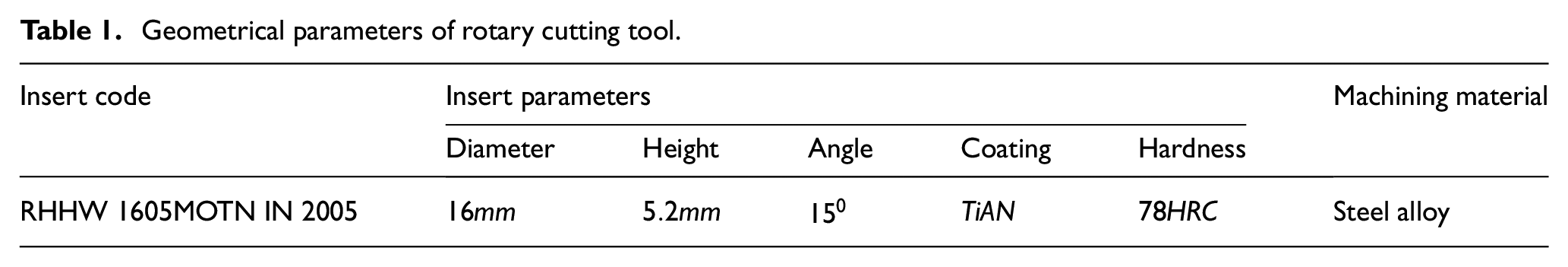
Experiments are designed with four input parameters including tool axis tilt angle $θ (\deg)$ , depth of cut $a_{p} (mm)$ , feed rate $f_{r} (mm / rev)$ , and cutting speed $v_{c} (m / min)$ with output parameter being surface roughness in hard turning 40X steel with achieve hardness $45 HRC$ on EMCOTURN E45 with C axis lathe machine. The experiments used INGERSOLL RHHW1605MOTN IN 2005 rotary cutting tool with geometrical parameters as shown in Table 1.

Table 1.

Geometrical parameters of rotary cutting tool.

Insert code	Insert parameters					Machining material
Insert code	Diameter	Height	Angle	Coating	Hardness	Machining material
RHHW 1605MOTN IN 2005	$16 mm$	$5.2 mm$	$15^{0}$	$TiAN$	$78 HRC$	Steel alloy

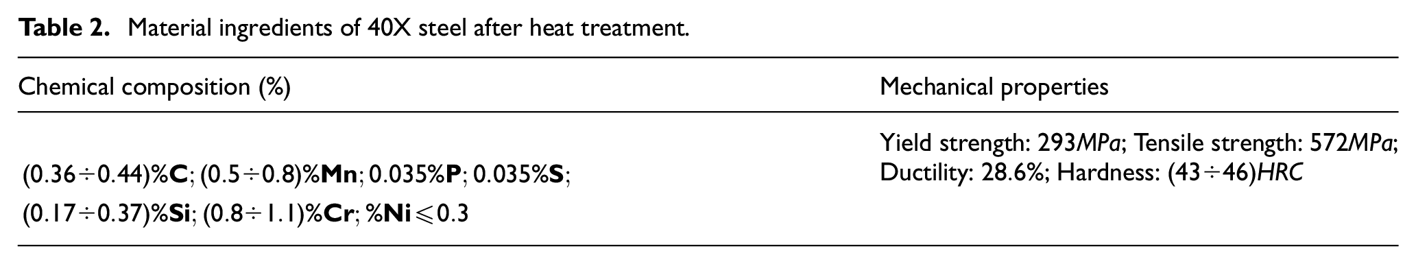
The ingredients and mechanical properties off 40X steel after heat treatment are shown in Table 2.

Table 2.

Material ingredients of 40X steel after heat treatment.

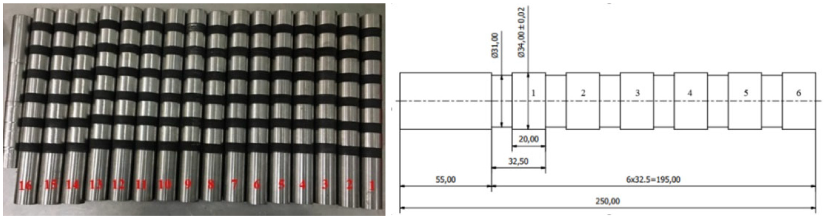
Chemical composition (%)	Mechanical properties
$\begin{matrix} (0.36 \div 0.44) % C; (0.5 \div 0.8) % Mn; 0.035 % P; 0.035 % S; \\ (0.17 \div 0.37) % Si; (0.8 \div 1.1) % Cr; % Ni \leq 0.3 \end{matrix}$	Yield strength: $293 MPa$ ; Tensile strength: $572 MPa$ ;Ductility: $28.6 %$ ; Hardness: $(43 \div 46) HRC$

Each workpiece is designed for performing $6 Ep$ with different input parameters (each workpiece segment is a set of input parameters) (Figure 1).

Figure 1.

40X steel workpiece and complete product.

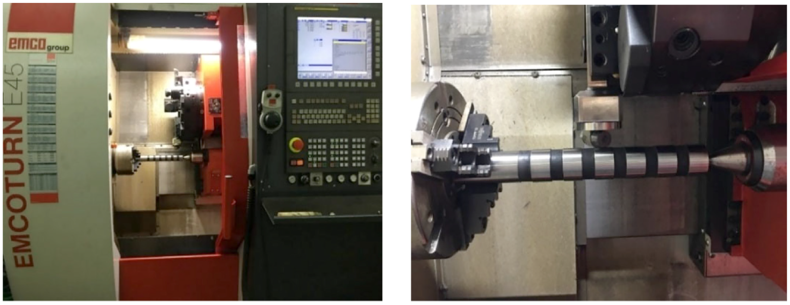
Steel workpiece and lathe machine in the experiments are depicted in Figure 2.

Figure 2.

Experimental model.

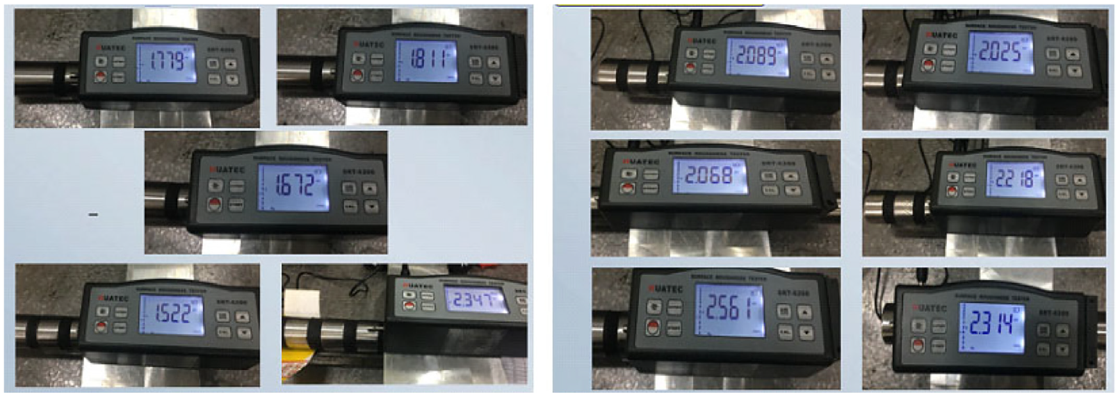
The roughness measuring device is a HUATEC SRT-6200 tester. Each position was measured three times. The final value is the average of three measurements. Some illustrative measurement results are shown in Figure 3.

Figure 3.

$SR$ measurement results.

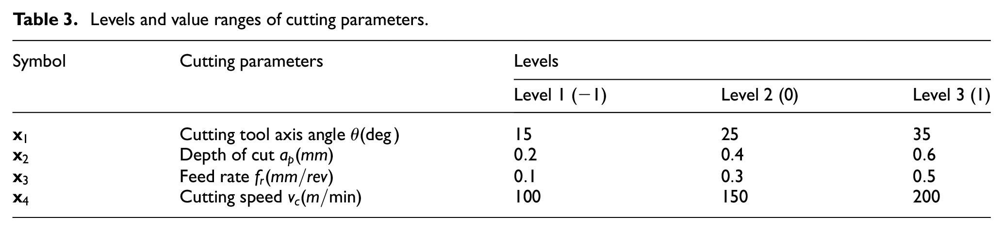
The range of cutting parameter variables utilized in the experiment was selected according to the cutting tool manufacturer’s recommendations and derived from the baseline experiments. Furthermore, a number of other criteria are used to select suitable cutting parameters including the hardness of the part, the turning process (finishing), and the residue left after semi-finishing. Table 3 shows the range of cutting parameters values.

Table 3.

Levels and value ranges of cutting parameters.

Symbol	Cutting parameters	Levels
Symbol	Cutting parameters	Level 1 (−1)	Level 2 (0)	Level 3 (1)
$x_{1}$	Cutting tool axis angle $θ (\deg)$	$15$	$25$	$35$
$x_{2}$	Depth of cut $a_{p} (mm)$	$0.2$	$0.4$	$0.6$
$x_{3}$	Feed rate $f_{r} (mm / rev)$	$0.1$	$0.3$	$0.5$
$x_{4}$	Cutting speed $v_{c} (m / min)$	$100$	$150$	$200$

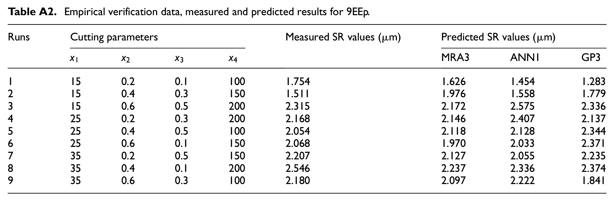
The number of $Ep$ to establish the regression model by $MRA, ANN$ , and $GP$ methods is $54 Ep$ . In order to more comprehensively assess the regression models, nine independent experiments were designed and processed according to Taguchi’s orthogonal experimental method,^6,8,26,36 with orthogonal arrays L₉. The experimental values dataset and the predicted values of the corresponding regression models are shown in detail in the Appendix Section with Tables A1 (for $54 Ep$ ) and A2 (for $9 EEp$ ).

The criteria for evaluating the regression models

Predictive models based on $MRA, ANN$ , and $GP$ techniques all have specific assessment criteria for model performance, accuracy, and reliability. These indicators include $R^{2}$ ,^13,18,36,37 $MSE$ ,¹⁹ $RMSE$ ,²⁰ and $MAPE$ .^21,27

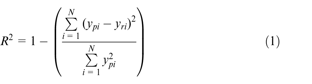
The $R^{2}$ value represents the suitability of the predicted values with the experimental data. Furthermore, this value also represents the change of the dependent variables that have been taken into account. The expression defining $R^{2}$ is described as follows

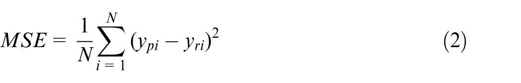
R^{2} = 1 - (\frac{\sum_{i = 1}^{N} {(y_{p i} - y_{r i})}^{2}}{\sum_{i = 1}^{N} y_{p i}^{2}})

(1)

The $MSE$ is a risk function and allows the determination of the mean squared difference between the predicted and the experimental values. The expression of the $MSE$ is presented as follows

MSE = \frac{1}{N} \sum_{i = 1}^{N} {(y_{pi} - y_{ri})}^{2}

(2)

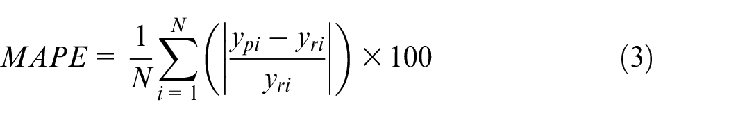
The $MAPE$ value entitles to estimate the deviation (in percentage) between the predicted value and the actual measured value. The expression for determining $MAPE$ is defined as follows

MAPE = \frac{1}{N} \sum_{i = 1}^{N} (| \frac{y_{pi} - y_{ri}}{y_{ri}} |) \times 100

(3)

where, $y_{pi}$ and $y_{ri}$ are the predicted values from the model and the values measured in the $i^{th}$ experiment, respectively. $N$ is the number of experiments. The $R^{2}$ , $MSE$ , and $MAPE$ criteria were utilized to assess the prediction models in this study.

The MRA, ANN, and GP methods

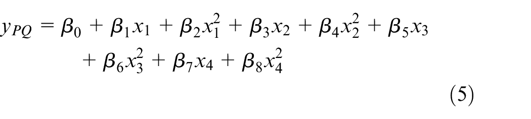
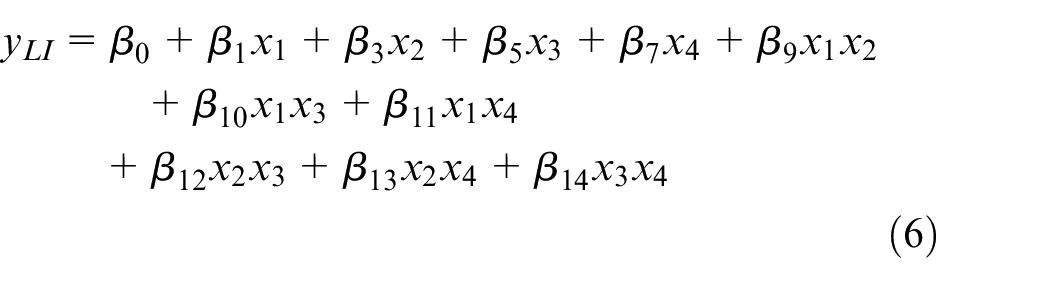
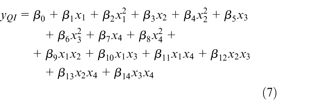
Four types of $MRA$ models are considered in this paper including Pure Linear ( $MRA 1$ ), Pure Quadratic ( $MRA 2$ ) polynomial, Linear Interactive ( $MRA 3$ ), and Interactive Quadratic ( $MRA 4$ ) order polynomials. These models are built based on finding out the significant regression coefficients for each specific $MRA$ model. The p-value is less than the significance level of 0.05.

The $MRA 1$ is described in detail as follows

y_{PL} = β_{0} + β_{1} x_{1} + β_{3} x_{2} + β_{5} x_{3} + β_{7} x_{4}

(4)

The $MRA 2$ is written as

\begin{matrix} y_{PQ} = β_{0} + β_{1} x_{1} + β_{2} x_{1}^{2} + β_{3} x_{2} + β_{4} x_{2}^{2} + β_{5} x_{3} \\ + β_{6} x_{3}^{2} + β_{7} x_{4} + β_{8} x_{4}^{2} \end{matrix}

(5)

The $MRA 3$ is considered as follows

\begin{matrix} y_{LI} = β_{0} + β_{1} x_{1} + β_{3} x_{2} + β_{5} x_{3} + β_{7} x_{4} + β_{9} x_{1} x_{2} \\ + β_{10} x_{1} x_{3} + β_{11} x_{1} x_{4} \\ + β_{12} x_{2} x_{3} + β_{13} x_{2} x_{4} + β_{14} x_{3} x_{4} \end{matrix}

(6)

Finally, the form of the $MRA 4$ regression equation is expressed as follows

\begin{matrix} y_{QI} = β_{0} + β_{1} x_{1} + β_{2} x_{1}^{2} + β_{3} x_{2} + β_{4} x_{2}^{2} + β_{5} x_{3} \\ + β_{6} x_{3}^{2} + β_{7} x_{4} + β_{8} x_{4}^{2} + \\ + β_{9} x_{1} x_{2} + β_{10} x_{1} x_{3} + β_{11} x_{1} x_{4} + β_{12} x_{2} x_{3} \\ + β_{13} x_{2} x_{4} + β_{14} x_{3} x_{4} \end{matrix}

(7)

Where, the regression coefficients $β_{i}, i = 0, . ., 14$ are undetermined. $y_{MRA 1}, y_{MRA 2}, y_{MRA 3}$ , and $y_{MRA 4}$ are the predicted objective function values, respectively; $x_{1}, x_{2}, x_{3}$ , and $x_{4}$ are the input variables.

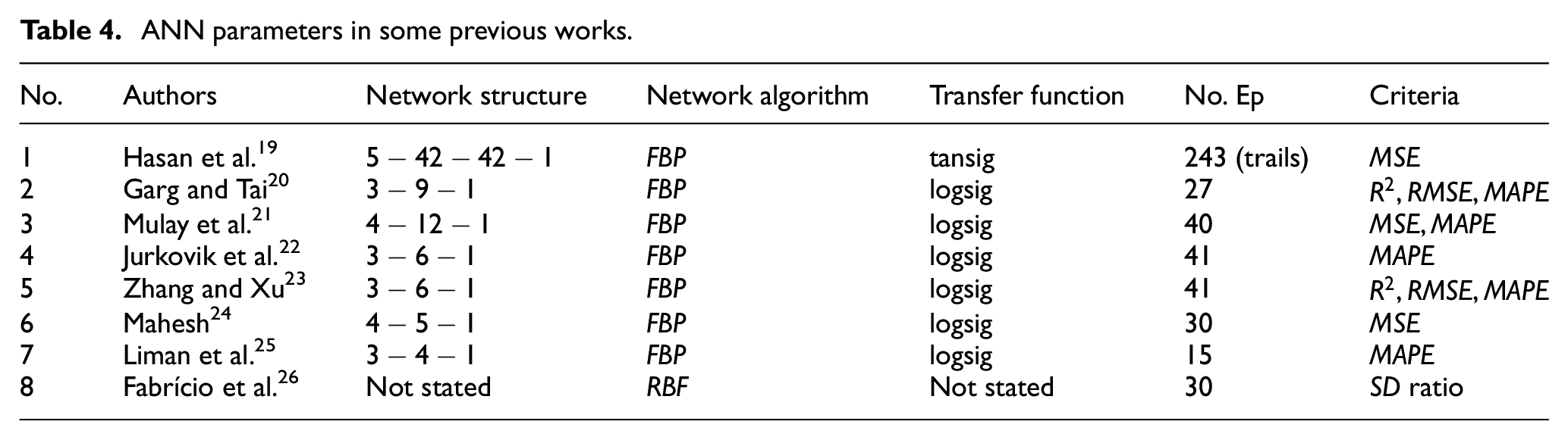
The main parameters in the $ANN$ structure of some previous works can be briefly summarized in Table 4.

Table 4.

ANN parameters in some previous works.

No.	Authors	Network structure	Network algorithm	Transfer function	No. Ep	Criteria
1	Hasan et al.¹⁹	$5 - 42 - 42 - 1$	$FBP$	tansig	$243$ (trails)	$MSE$
2	Garg and Tai²⁰	$3 - 9 - 1$	$FBP$	logsig	$27$	$R^{2}, RMSE, MAPE$
3	Mulay et al.²¹	$4 - 12 - 1$	$FBP$	logsig	$40$	$MSE, MAPE$
4	Jurkovik et al.²²	$3 - 6 - 1$	$FBP$	logsig	$41$	$MAPE$
5	Zhang and Xu²³	$3 - 6 - 1$	$FBP$	logsig	$41$	$R^{2}, RMSE, MAPE$
6	Mahesh²⁴	$4 - 5 - 1$	$FBP$	logsig	$30$	$MSE$
7	Liman et al.²⁵	$3 - 4 - 1$	$FBP$	logsig	$15$	$MAPE$
8	Fabrício et al.²⁶	Not stated	$RBF$	Not stated	$30$	$SD$ ratio

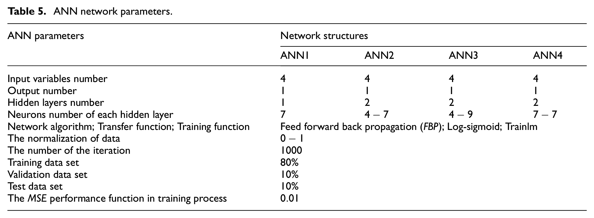
Based on Table 4 and the results of proposing the number of neurons in each hidden layer in Zhang et al.,³⁸ four $ANN$ structures have been implemented in this study to select the appropriate $ANN$ model best. Whereby, $ANN 1$ network has three layers including one input layer (four parameters), one hidden layer (seven neurons), and one output layer (one parameter). The $ANN 1$ network can be denoted as $4 - 7 - 1$ . Similarly, structures and parameters of other models are described in Table 5. The training process control error value used is $MSE$ . The normalized $MSE$ value is 0.01.

Table 5.

ANN network parameters.

$ANN$ parameters	Network structures
$ANN$ parameters	$ANN 1$	$ANN 2$	$ANN 3$	$ANN 4$
Input variables number	$4$	$4$	$4$	$4$
Output number	$1$	$1$	$1$	$1$
Hidden layers number	$1$	$2$	$2$	$2$
Neurons number of each hidden layer	$7$	$4 - 7$	$4 - 9$	$7 - 7$
Network algorithm; Transfer function; Training function	Feed forward back propagation ( $FBP$ ); Log-sigmoid; Trainlm
The normalization of data	$0 - 1$
The number of the iteration	$1000$
Training data set	$80 %$
Validation data set	$10 %$
Test data set	$10 %$
The $MSE$ performance function in training process	$0.01$

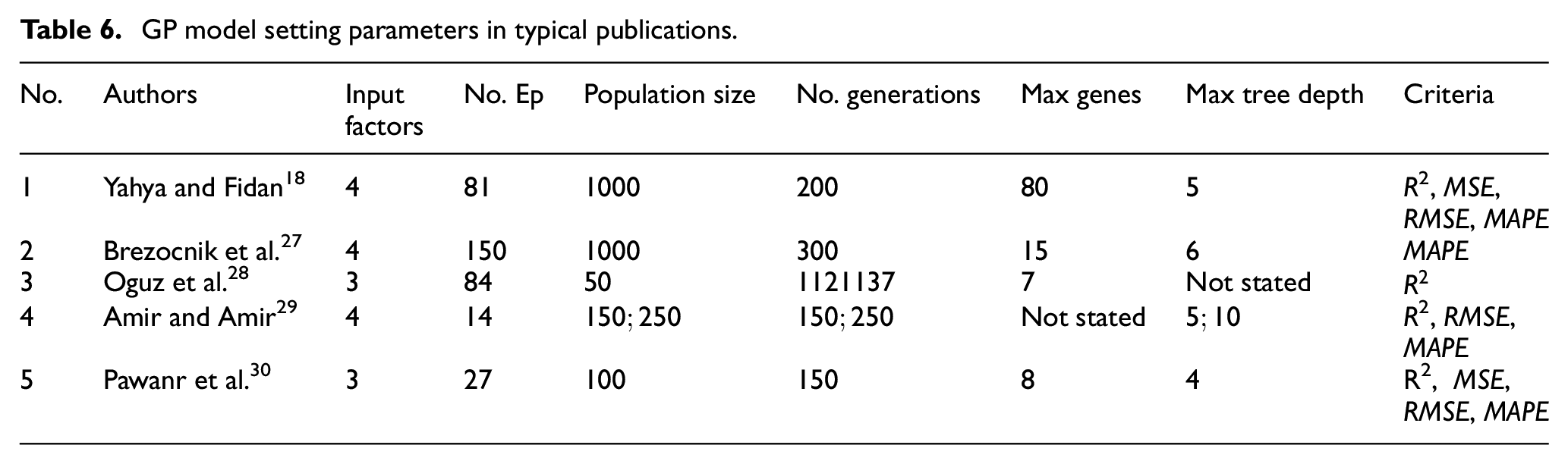
The main parameters to set up the $GP$ method in such typical works is described in detail in Table 6. The $MSE$ target value for the loop response during training the models to find the most suitable regression equation does not exceed 0.02.

Table 6.

GP model setting parameters in typical publications.

No.	Authors	Input factors	No. Ep	Population size	No. generations	Max genes	Max tree depth	Criteria
1	Yahya and Fidan¹⁸	$4$	$81$	$1000$	$200$	$80$	$5$	R ², MSE,RMSE, MAPE
2	Brezocnik et al.²⁷	$4$	$150$	$1000$	$300$	$15$	$6$	$MAPE$
3	Oguz et al.²⁸	$3$	$84$	$50$	$1121137$	$7$	Not stated	$R^{2}$
4	Amir and Amir²⁹	$4$	$14$	$150; 250$	$150; 250$	Not stated	$5; 10$	R ², RMSE,MAPE
5	Pawanr et al.³⁰	$3$	$27$	$100$	$150$	$8$	$4$	R², MSE,RMSE, MAPE

Similar to the $ANN$ selection, three models $GP 1, GP 2$ , and $GP 3$ are proposed to be implemented in this study with different set of parameters.

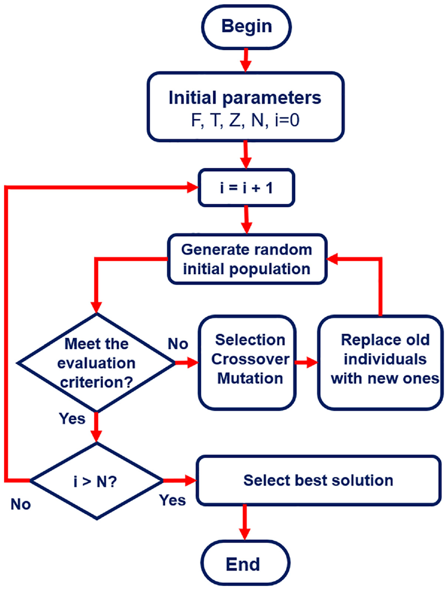
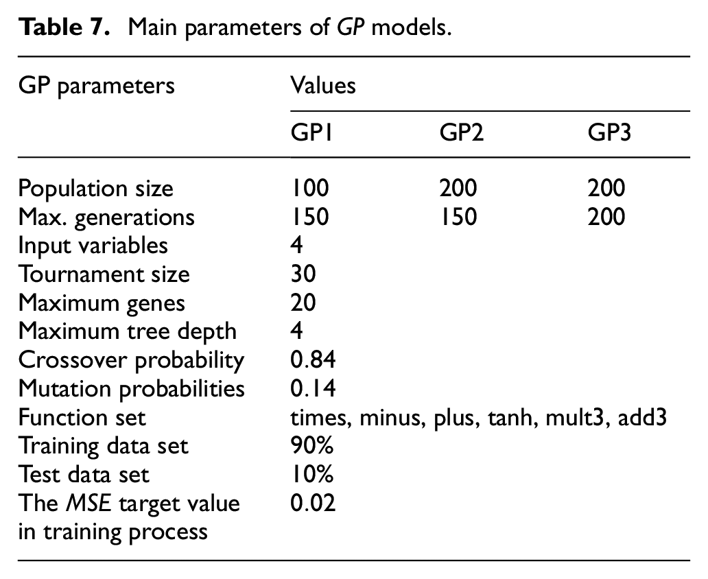
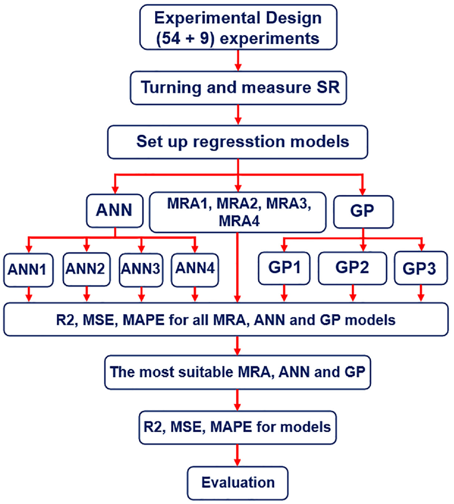
Figure 4 describes the steps to implement the $GP$ algorithm. In which, $F = {+, -, *, /, mult 3, add 3, . . .}$ is the set of functional genes, $T = {x_{1}, x_{2}, x_{3}, x_{4}}$ is the set of terminal genes, and $Z$ is the set of arguments corresponding to the set of $F$ ,^34,35 and $N$ is the number of generations. Table 7 shows the basic parameters of the GP models.

Figure 4.

Algorithm implementation steps in $GP$ .

Table 7.

Main parameters of $GP$ models.

GP parameters	Values
GP parameters	$GP 1$	$GP 2$	$GP 3$
Population size	$100$	$200$	$200$
Max. generations	$150$	$150$	$200$
Input variables	$4$
Tournament size	$30$
Maximum genes	$20$
Maximum tree depth	$4$
Crossover probability	$0.84$
Mutation probabilities	$0.14$
Function set	times, minus, plus, tanh, mult3, add3
Training data set	$90 %$
Test data set	$10 %$
The $MSE$ target value in training process	$0.02$

After performing experiments and collecting the results, the calculation is carried out according to the steps that are shown in Figure 5.

Figure 5.

Implementation steps.

Analysis results and discussion

Prediction models of $SR$ values by $MRA, ANN$ , and $GP$ methods are established based on experimental results described in Appendix.

Prediction results of MRA method

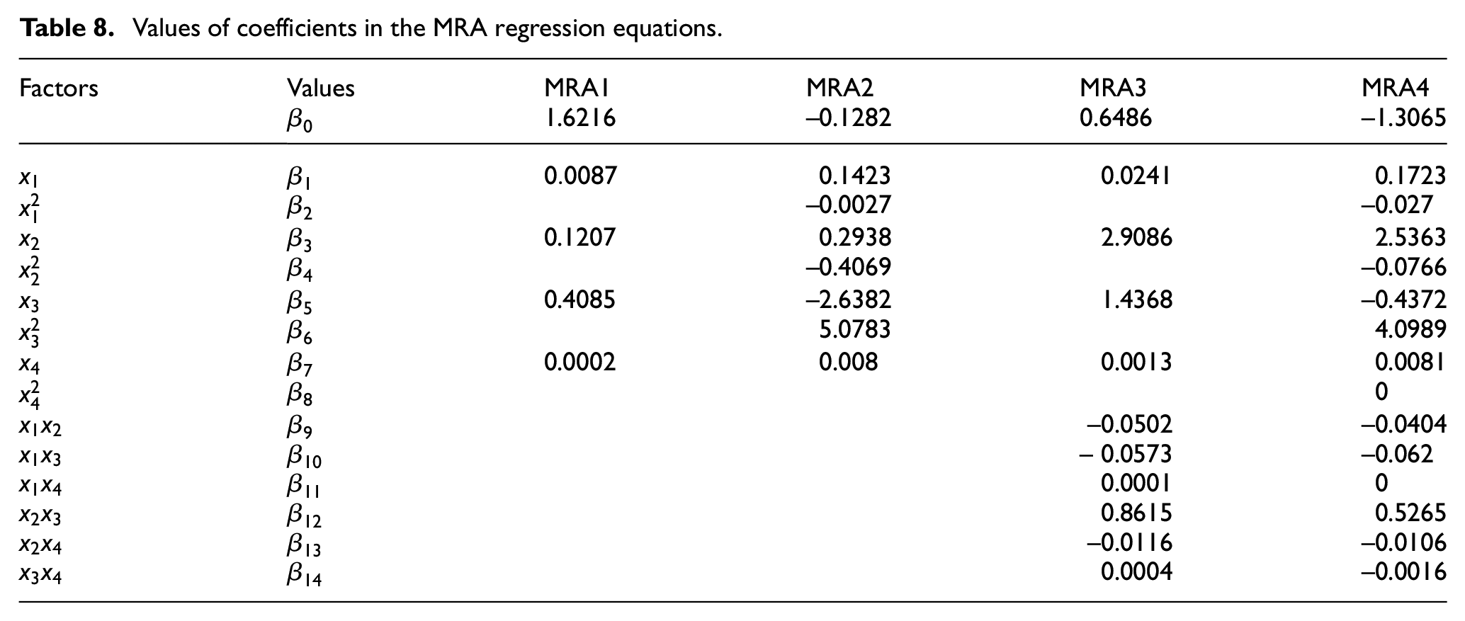
The determination of the regression coefficients is done through the data collected in $54 Ep$ and the $MRA$ theory based on the four $MRA$ models considered above. Calculation results of regression coefficients corresponding to each type of equation are described in detail in Table 8.

Table 8.

Values of coefficients in the MRA regression equations.

Factors	Values	$MRA 1$	$MRA 2$	$MRA 3$	$MRA 4$
Factors	$β_{0}$	1.6216	–0.1282	0.6486	–1.3065
$x_{1}$	$β_{1}$	$0.0087$	0.1423	0.0241	0.1723
$x_{1}^{2}$	$β_{2}$		–0.0027		–0.027
$x_{2}$	$β_{3}$	0.1207	0.2938	2.9086	2.5363
$x_{2}^{2}$	$β_{4}$		–0.4069		–0.0766
$x_{3}$	$β_{5}$	0.4085	–2.6382	1.4368	–0.4372
$x_{3}^{2}$	$β_{6}$		5.0783		4.0989
$x_{4}$	$β_{7}$	0.0002	0.008	0.0013	0.0081
$x_{4}^{2}$	$β_{8}$				$0$
$x_{1} x_{2}$	$β_{9}$			–0.0502	–0.0404
$x_{1} x_{3}$	$β_{10}$			– 0.0573	–0.062
$x_{1} x_{4}$	$β_{11}$			0.0001	0
$x_{2} x_{3}$	$β_{12}$			0.8615	0.5265
$x_{2} x_{4}$	$β_{13}$			–0.0116	–0.0106
$x_{3} x_{4}$	$β_{14}$			0.0004	–0.0016

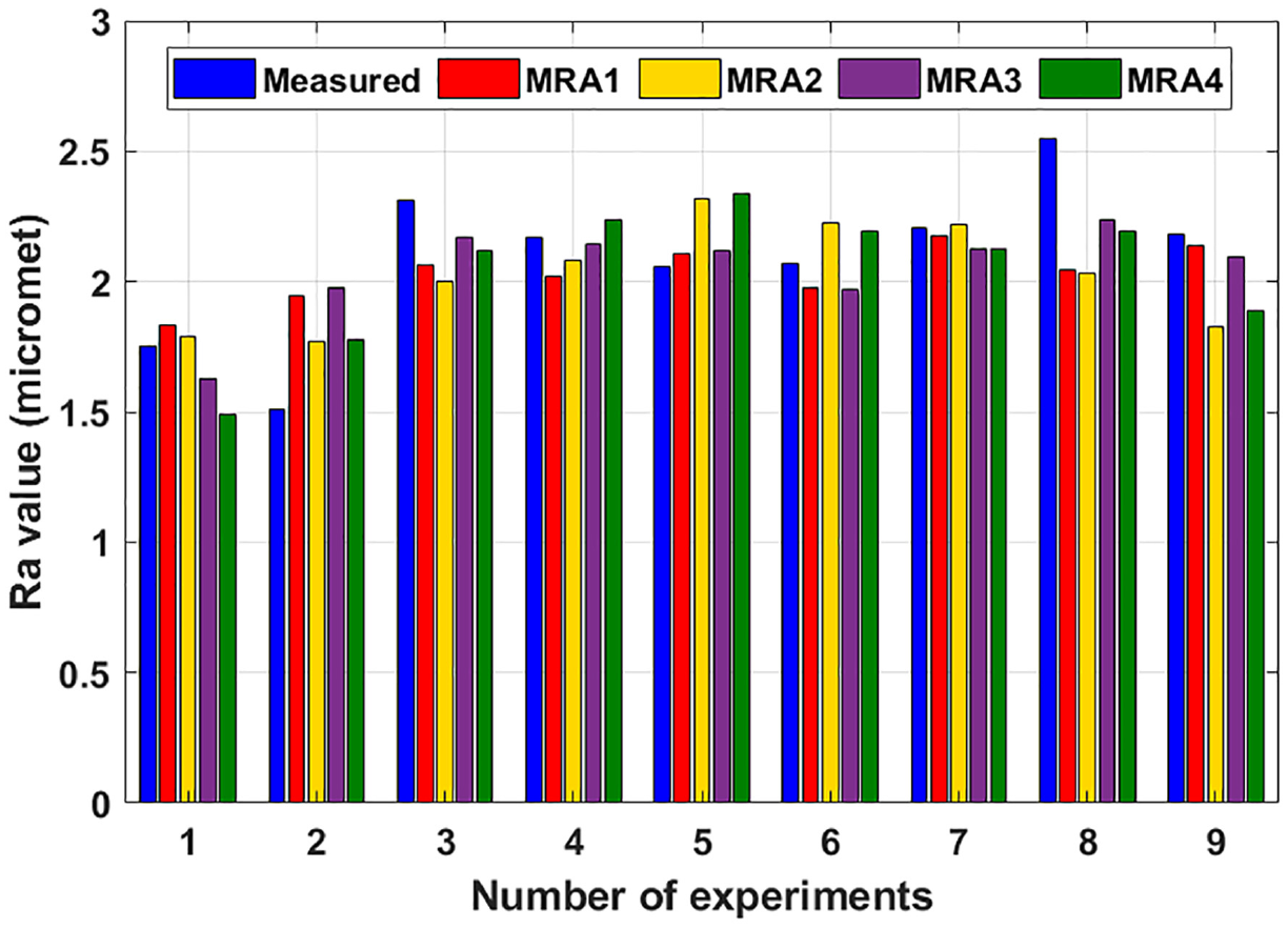
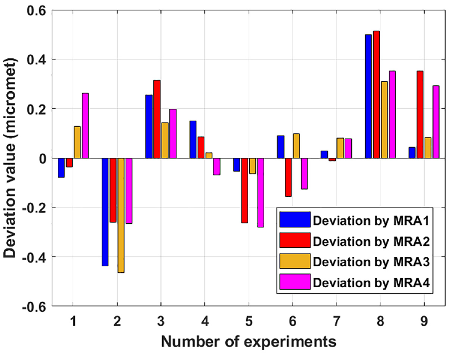
According to the data in Table 8, the regression equations are established. The comparison of the prediction results of the $MRA$ models with the values measured in $9 EEp$ is shown in Figure 6. The deviations of the predicted values from reality are shown in Figure 7.

Figure 6.

Comparison of prediction results of $MRA$ models in $9 EEp$ .

Figure 7.

Predicted value deviation of $MRA$ models in $9 EEp$ .

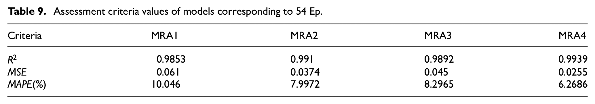
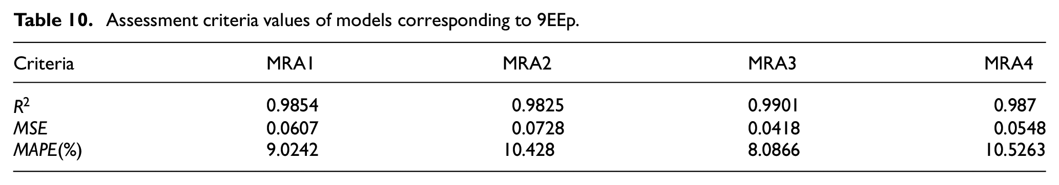
The criteria values to evaluate the accuracy and reliability of the $MRA$ models corresponding to $54 Ep$ and $9 EEp$ are described in Tables 9 and 10, respectively.

Table 9.

Assessment criteria values of models corresponding to 54 Ep.

Criteria	$MRA 1$	$MRA 2$	$MRA 3$	$MRA 4$
$R^{2}$	0.9853	0.991	0.9892	0.9939
$MSE$	0.061	0.0374	0.045	0.0255
$MAPE (%)$	10.046	7.9972	8.2965	6.2686

Table 10.

Assessment criteria values of models corresponding to $9 EEp$ .

Criteria	$MRA 1$	$MRA 2$	$MRA 3$	$MRA 4$
$R^{2}$	0.9854	0.9825	0.9901	0.987
$MSE$	0.0607	0.0728	0.0418	0.0548
$MAPE (%)$	9.0242	10.428	8.0866	10.5263

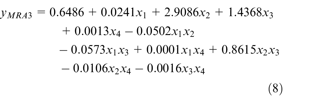
In Table 9, most of the models have $R^{2}$ values above $0.98$ , showing the high reliability of the regression models. The $MRA 4$ model has the smallest $MSE$ and $MAPE$ errors of $0.026$ and 6.269%, respectively. However, Table 10 shows that the prediction criteria of the $MRA 3$ model gave the best results with $R^{2}$ of $0.99$ , $MSE$ of $0.042$ , and $MAPE$ of $8.087 %$ . Based on the above results, the $MRA 3$ regression model was selected as the most suitable model among the considered models. The $MRA 3$ regression equation corresponding to the coefficients in Table 8 is shown as follows

\begin{matrix} y_{MRA 3} = 0.6486 + 0.0241 x_{1} + 2.9086 x_{2} + 1.4368 x_{3} \\ + 0.0013 x_{4} - 0.0502 x_{1} x_{2} \\ - 0.0573 x_{1} x_{3} + 0.0001 x_{1} x_{4} + 0.8615 x_{2} x_{3} \\ - 0.0106 x_{2} x_{4} - 0.0016 x_{3} x_{4} \end{matrix}

(8)

Where, angle of cutting tool axis $x_{1} = θ (\deg)$ , depth of cut $x_{2} = a_{p} (mm)$ , feed rate $x_{3} = f_{r} (mm / rev)$ , and cutting speed $x_{4} = v_{c} (m / min)$ . The $MRA 3$ model and the evaluation parameters in Tables 9 and 10 are used to assess with the regression model from the $ANN$ and $GP$ method below. $SR$ prediction results of the $MRA 3$ model with $54 Ep$ is described in Figure 8.

Figure 8.

$SR$ prediction results of the $MRA 3$ model with $54 Ep$ .

Prediction results of ANN method

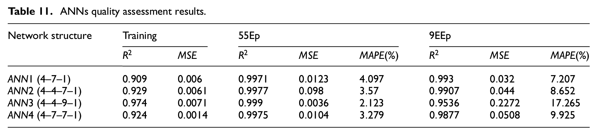
The estimation criteria of $ANN$ models during training, prediction value $54 Ep$ and $9 EEp$ are shown in Table 11.

Table 11.

ANNs quality assessment results.

Network structure	Training		$55 Ep$			$9 EEp$
Network structure	$R^{2}$	$MSE$	$R^{2}$	$MSE$	$MAPE (%)$	$R^{2}$	$MSE$	$MAPE (%)$
$ANN 1$ (4–7–1)	$0.909$	$0.006$	$0.9971$	$0.0123$	$4.097$	$0.993$	$0.032$	$7.207$
$ANN 2$ (4–4–7–1)	$0.929$	$0.0061$	$0.9977$	$0.098$	$3.57$	$0.9907$	$0.044$	$8.652$
$ANN 3$ (4–4–9–1)	$0.974$	$0.0071$	$0.999$	$0.0036$	$2.123$	$0.9536$	$0.2272$	$17.265$
$ANN 4$ (4–7–7–1)	$0.924$	$0.0014$	$0.9975$	$0.0104$	$3.279$	$0.9877$	$0.0508$	$9.925$

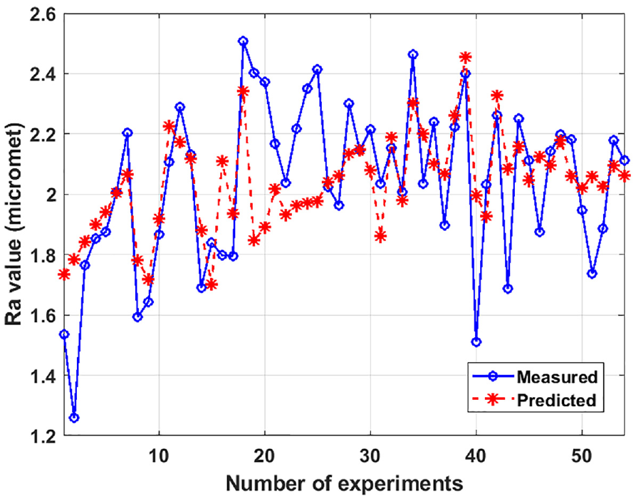
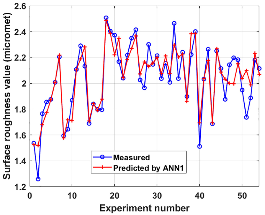
For the training results, the $ANN 3$ network gives the highest $R^{2}$ value ( $0.974$ ). The $MSE$ value of $ANN 4$ is the smallest ( $0.0014$ ). For the prediction results of $54 Ep$ , the $R^{2}$ values of all $ANN$ models are above $0.997$ . The $MSE$ value of $ANN 3$ is the lowest ( $0.0036$ ). However, the results of predicting $9 EEp$ (as an objective test), the $ANN 1$ gives the most reliable assessment criteria with $R^{2}$ being the largest ( $0.993$ ). The $MSE$ ( $0.032$ ) and $MAPE$ ( $7.207 %$ ) values are the smallest. Accordingly, the $ANN 1$ model was selected as the more suitable model than other ones. $ANN 1$ is used to compare with the $MRA$ and $GP$ models. Figure 9 shows the comparison results between the predicted value of the $ANN 1$ and the actual measured value in $54 Ep$ .

Figure 9.

$SR$ values predicted by ANN1 (4–7–1) in $54 Ep$ .

Prediction results for GP method

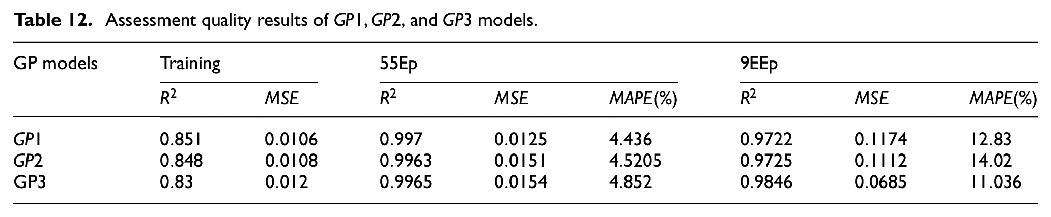
$GP$ models were performed in the MATLAB environment for two cases (dataset for $54 Ep$ and dataset for $9 EEp$ ). The results of predicting $SR$ values for $GP$ models are presented in detail in Appendix. The calculation results of the criteria are described in Table 12.

Table 12.

Assessment quality results of $GP 1, GP 2$ , and $GP 3$ models.

$GP$ models	Training		$55 Ep$			$9 EEp$
$GP$ models	$R^{2}$	$MSE$	$R^{2}$	$MSE$	$MAPE (%)$	$R^{2}$	$MSE$	$MAPE (%)$
$GP 1$	$0.851$	$0.0106$	$0.997$	$0.0125$	$4.436$	$0.9722$	$0.1174$	$12.83$
$GP 2$	$0.848$	$0.0108$	$0.9963$	$0.0151$	$4.5205$	$0.9725$	$0.1112$	$14.02$
$GP 3$	$0.83$	$0.012$	$0.9965$	$0.0154$	$4.852$	$0.9846$	$0.0685$	$11.036$

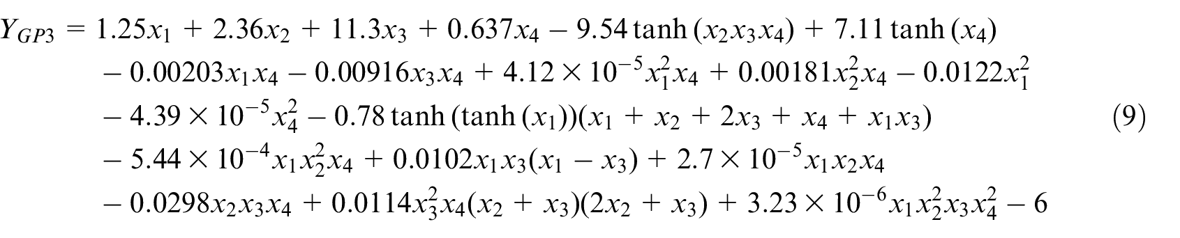
Regarding the training results, the $GP 1$ model gave a higher $R^{2}$ value (0.851) than the other two models ( $0.848$ and $0.83$ ). The $MSE$ error value ( $0.0106$ ) of $GP 1$ is the lowest. Similarly, the prediction results corresponding to $54 Ep$ , the criteria values of the $GP 2$ and $GP 3$ models are lower than the $GP 1$ model. However, it can be noticed that the values of the indicators have extremely minor difference. Furthermore, in the $9 EEp$ prediction dataset, the $GP 3$ model gave the best results, the $R^{2}$ value ( $0.9846$ ) showed higher reliability, the $MSE$ value ( $0.0685$ ), and $MAPE$ value ( $11.036 %$ ) tremendously lower than $GP 1, GP 2$ . The $GP 3$ model can be considered as the most feasible. This model was chosen to compare the prediction performance with the $MRA$ and $ANN 1$ models. The regression equation corresponding to the $GP 3$ model has the form as follows

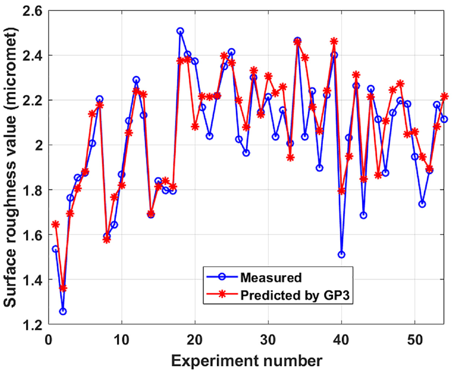
\begin{matrix} Y_{GP 3} = 1.25 x_{1} + 2.36 x_{2} + 11.3 x_{3} + 0.637 x_{4} - 9.54 \tanh (x_{2} x_{3} x_{4}) + 7.11 \tanh (x_{4}) \\ \begin{matrix}  \end{matrix} - 0.00203 x_{1} x_{4} - 0.00916 x_{3} x_{4} + 4.12 \times 10^{- 5} x_{1}^{2} x_{4} + 0.00181 x_{2}^{2} x_{4} - 0.0122 x_{1}^{2} \\ \begin{matrix}  \end{matrix} - 4.39 \times 10^{- 5} x_{4}^{2} - 0.78 \tanh (\tanh (x_{1})) (x_{1} + x_{2} + 2 x_{3} + x_{4} + x_{1} x_{3}) \\ \begin{matrix}  \end{matrix} - 5.44 \times 10^{- 4} x_{1} x_{2}^{2} x_{4} + 0.0102 x_{1} x_{3} (x_{1} - x_{3}) + 2.7 \times 10^{- 5} x_{1} x_{2} x_{4} \\ \begin{matrix}  \end{matrix} - 0.0298 x_{2} x_{3} x_{4} + 0.0114 x_{3}^{2} x_{4} (x_{2} + x_{3}) (2 x_{2} + x_{3}) + 3.23 \times 10^{- 6} x_{1} x_{2}^{2} x_{3} x_{4}^{2} - 6 \end{matrix}

(9)

The results of the comparison between the predicted values and the actual measured data are shown in Figure 10.

Figure 10.

$SR$ value predicted by $GP 3$ in $54 Ep$ .

Overall assessment

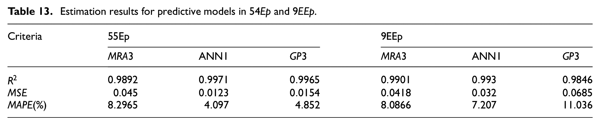
The criteria for appraising the prediction results from $54 Ep$ and $9 EEp$ by $MRA 3, ANN 1$ , and $GP 3$ regression models are shown in Table 13.

Table 13.

Estimation results for predictive models in $54 Ep$ and $9 EEp$ .

Criteria	$55 Ep$			$9 EEp$
Criteria	$MRA 3$	$ANN 1$	$GP 3$	$MRA 3$	$ANN 1$	$GP 3$
$R^{2}$	$0.9892$	$0.9971$	$0.9965$	$0.9901$	$0.993$	$0.9846$
$MSE$	$0.045$	$0.0123$	$0.0154$	$0.0418$	$0.032$	$0.0685$
$MAPE (%)$	$8.2965$	$4.097$	$4.852$	$8.0866$	$7.207$	$11.036$

For $54 Ep$ , the $ANN 1$ model achieves the largest $R^{2}$ value ( $0.9971$ ) and the $MRA 3$ is lowest ( $0.989$ ) in this case. Accordingly, the $MSE$ value of the $MRA 3$ model is the largest ( $0.045$ ), the smallest value belongs to the $ANN 1$ model ( $0.0123$ ). The $MAPE$ value compared with actual values is the most reliable $ANN 1$ method ( $4.097 %$ ), then $GP 3$ method ( $4.852 %$ ) and finally $MRA 3$ ( $8.296 %$ ). The $MSE$ and $MAPE$ values of the $MRA 3$ model are higher than those of $ANN 1$ and $GP 3$ in this case. Therefore, the prediction accuracy of $MRA 3$ is not as high as that of $ANN 1$ and $GP 3$ .

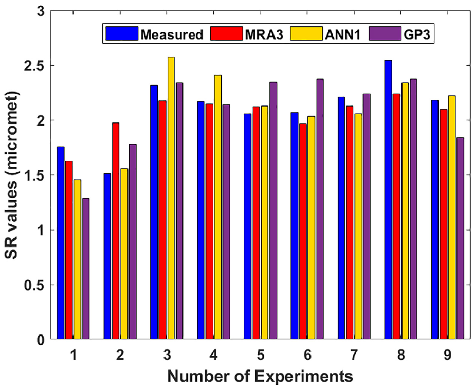
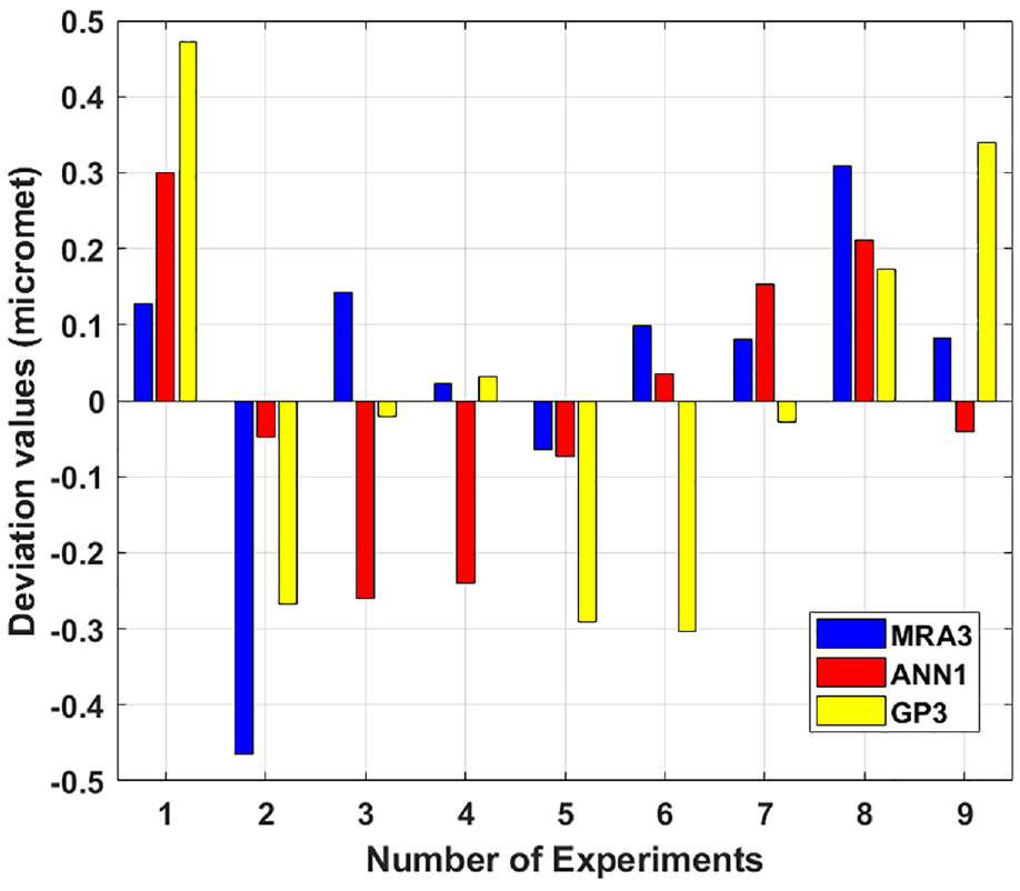
For $9 EEp$ , the evaluation criteria of the $ANN 1$ model are the best with the smallest $MSE$ ( $0.032$ ) and $MAPE$ ( $7.207 %$ ). The $MRA 3$ and $GP 3$ have a lower confidence predictive criteria value than the $ANN 1$ model, but the $R^{2}$ values are not too different. The deviation between the values of $MRA 3$ and $ANN 1$ is quite large with $MSE$ ( $0.0418; 0.032$ ) and $MAPE$ ( $8.086 %; 7.207 %$ ) although these models describe the high nonlinearity of the system. The difference between the measured $SR$ value and the predicted value by the $MRA 3, ANN 1$ , and $GP 3$ regression models is shown in Figure 11. The distribution of deviations of the predicted values from reality is described in Figure 12. The maximum deviation value is close to $0.5 μ m$ .

Figure 11.

Compare the $SR$ value between reality and prediction.

Figure 12.

Deviation value $SR$ of methods compared with reality.

Conclusion

This paper presents the results of building predictive models of surface roughness values based on hard turning experiments with self-rotating cutting tools for 40X materials on CNC lathes with C axis. The novelty in this study in terms of method and machinability is reflected in a number of points as follows:

Three statistical research methods including $MRA, ANN$ , and $GP$ are specifically considered in this study. The effectiveness of each method for a statistical object is compared with specific criteria. For each method applied at least three mathematical models are specifically considered (four $MRA$ models, four $ANN$ models, three $GP$ models). The most suitable $MRA 3, ANN 1$ , and $GP 3$ models are selected from comparing the results of estimating $MRAi, (i = 1, . ., 4)$ , $ANNi, (i = 1, . ., 4)$ , and $GPi, (i = 1, 2, 3)$ models. Based on the prediction results of nine independent EEp after building regression models, the prediction criteria of the $MRA 3$ model gave the best results in four $MRA$ models with $R^{2} (0.99)$ , $MSE (0.042)$ , and $MAPE (8.087 %)$ . The $ANN 1$ gives the most reliable assessment criteria in four $ANN$ models with $R^{2} (0.993)$ being the largest. The $MSE (0.032)$ and $MAPE (7.207 %)$ values are the smallest. The $GP 3$ model gave the best in three $GP$ models with $R^{2} (0.9846)$ , $MSE (0.0685)$ , and $MAPE (11.036 %)$ . The results of predicting the $SR$ value between the selected $MRA, ANN$ , and $GP$ models will be assessed in detail. Accordingly, the evaluation criteria of the $ANN 1$ model are the best with the smallest $MSE$ and $MAPE$ . The $MRA 3$ and $GP 3$ have a lower confidence predictive criteria value than the $ANN 1$ model. With a huge enough amount of data, the ANN method shows the highest efficiency. However, for the purpose of looking at the interplay effects between the parameters, the GP method is better suited. This result allows a reference to choose suitable model to use in similar studies. It should be noted that most of the previous publications only considered and applied a single statistical method. The mathematical model for that statistical method was chosen from the outset, and there was no specific comparison of the effectiveness between the mathematical models of the chosen method. Moreover, the grinding or polishing steps after turning process can be eliminated when the surface roughness meets the specified requirements. This helps to reduce machining costs.

The results of investigation methods with many different models can be used as a basis for selecting suitable prediction models according to the amount of data and the corresponding selection criteria as follows:

The linear model $MRA 1$ and $MRA 2$ can be applied when it is necessary to determine the influence of each independent variable on the objective function and high accuracy is not required.

$MRA$ models should be used when it is necessary to build a simple, fast, and efficient predictive model with a small amount of data. In contrast, the $ANN$ and $GP$ models are suitable for huge amounts of experimental data.

The $ANN$ and $GP$ models should be used when it is necessary to establish an interpolation model with high prediction accuracy and large amount of experimental data.

The $MRA 4, ANN$ , and $GP$ models should be used when it is necessary to accurately determine the influence of pairs of independent variables, taking into account the interaction between them or the relationship between the variables is complex and the nonlinearity is strong.

With the $ANN$ model, increasing the number of neurons in each hidden layer or increasing the number of hidden layers does not guarantee an increase in the accuracy of the prediction model.

It should be noted that product quality is assessed through $SR$ value, dimensional accuracy, relative position errors, and mechanical properties. Therefore, factors affecting those criteria such as cutting force, vibration, tool wear also need to be considered specifically. These problems will be further studied in the near future.

Footnotes

Appendix

Table A2.

Empirical verification data, measured and predicted results for $9 EEp$ .

Runs	Cutting parameters				Measured SR values (µm)	Predicted SR values (µm)
Runs	$x_{1}$	$x_{2}$	$x_{3}$	$x_{4}$	Measured SR values (µm)	MRA3	ANN1	GP3
1	15	0.2	0.1	100	1.754	1.626	1.454	1.283
2	15	0.4	0.3	150	1.511	1.976	1.558	1.779
3	15	0.6	0.5	200	2.315	2.172	2.575	2.336
4	25	0.2	0.3	200	2.168	2.146	2.407	2.137
5	25	0.4	0.5	100	2.054	2.118	2.128	2.344
6	25	0.6	0.1	150	2.068	1.970	2.033	2.371
7	35	0.2	0.5	150	2.207	2.127	2.055	2.235
8	35	0.4	0.1	200	2.546	2.237	2.336	2.374
9	35	0.6	0.3	100	2.180	2.097	2.222	1.841

Declaration of conflicting interests

The author declared no potential conflicts of interest with respect to the research, authorship, and/or publication of this article.

Funding

The author received no financial support for the research, authorship, and/or publication of this article.

ORCID iD

Duong Xuan Bien

References

Chang

Chen

Pang

, et al. Selection of cutting regime for self-propelled rotary cutting tools. Proc IMechE, Part B: J Engineering Manufacture 1995; 203: 63–66.

Kishawy

Becze

McIntosh

. Tool performance and attainable surface quality during the machining of aerospace alloys using self-propelled rotary tools. J Mater Process Technol 2004; 152: 266–271.

Ezugwu

Olajire

Wang

. Wear evaluation of a self-propelled rotary tool when machining titanium alloy IMI 318. Proc IMechE, Part B: J Engineering Manufacture 2002; 216(6): 891–897.

Thanh

Dung

Mia

. Multi-response optimization of the actively driven rotary turning for energy efficiency, carbon emissions, and machining quality. Proc IMechE, Part B: J Engineering Manufacture 2021; 235(13): 2155–2173.

Bartarya

Choudhury

. Influence of machining parameters on forces and surface roughness during finish hard turning of EN 31 steel. Proc IMechE, Part B: J Engineering Manufacture 2014; 228(9): 1068–1080.

Kam

Demirtas

. Analysis of tool vibration and surface roughness during turning process of tempered steel samples using Taguchi method. Proc IMechE, Part E: J Process Mechanical Engineering 2021; 235: 1429–1438.

Rashid

Goel

Luo

, et al. An experimental investigation for the improvement of attainable surface roughness during hard turning process. Proc IMechE, Part B: J Engineering Manufacture 2013; 227: 338–342.

Kam

. Effects of deep cryogenic treatment on machinability, hardness and microstructure in dry turning process of tempered steels. Proc IMechE, Part E: J Process Mechanical Engineering 2021; 235: 927–936.

Kam

Seremet

. Experimental investigation of the effect of machinability on surface quality and vibration in hard turning of hardened AISI 4140 steels using ceramic cutting tools. Proc IMechE, Part E: J Process Mechanical Engineering 2021; 235(5): 1565–1574.

10.

Imani

Henzaki

Hamzeloo

, et al. Modeling and optimizing of cutting force and surface roughness in milling process of Inconel 738 using hybrid ANN and GA. Proc IMechE, Part B: J Engineering Manufacture 2019; 234(5): 920–932.

11.

Bhardwaj

Kumar

Singh

. Surface roughness prediction model for turning of AISI 1019 steel using response surface methodology and Box–Cox transformation. Proc IMechE, Part B: J Engineering Manufacture 2014; 228(2): 223–232.

12.

Suresh

Rao

Deshmukh

. A genetic algorithmic approach for optimization of surface roughness prediction model. Int J Mach Tools Manuf 2002; 42: 675–680.

13.

Ilhan

Mehmet

. Modeling and prediction of surface roughness in turning operations using artificial neural network and multiple regression method. Expert Syst Appl 2011; 38: 5826–5832.

14.

Patel

Kiran

. A non-contact approach for surface roughness prediction in CNC turning using a linear regression model. Mater Today Proc 2022; 26: 350–355.

15.

Chen

Wang

Zhang

. Multiple regression prediction model for cutting forces and surface roughness in micro-milling of TA2. Procedia CIRP 2020; 89: 233–238.

16.

Choudhury

Das

Banpurkar

, et al. Regression analysis of wetting characteristics for different random surface roughness of polydimethylsiloxane using sandpapers. Colloids Surf A Physicochem Eng Asp 2022; 647: 129038.

17.

Ozel

Karpat

. Predictive modeling of surface roughness and tool wear in hard turning using regression and neural networks. Int J Mach Tools Manuf 2005; 45: 467–479.

18.

Yahya

Fidan

. Analysis of cutting parameters on tool wear in turning of Ti-6Al-4V alloy by multiple linear regression and genetic expression programming methods. Measurement 2022; 200: 111638.

19.

Hasan

Tuncay

Fehmi

. Prediction of minimum surface roughness in end milling mold parts using neural network and genetic algorithm. Mater Des 2006; 27: 735–744.

20.

Garg

Tai

. Stepwise approach for the evolution of generalized genetic programming model in prediction of surface finish of the turning process. Adv Eng Softw 2014; 78: 16–27.

21.

Mulay

Ben

Syed

, et al. Prediction of average surface roughness and formability in single point incremental forming using artificial neural network. Arch Civ Mech Eng 2019; 19: 1135–1149.

22.

Jurkovic

Cukor

Brezocnik

, et al. A comparison of machine learning methods for cutting parameters prediction in high-speed turning process. J Intell Manuf 2016; 29: 1683–1693.

23.

Zhang

. Machine learning cutting force, surface roughness, and tool life in high-speed turning processes. Manuf Lett 2021; 29: 84–89.

24.

Mahesh

. Prediction of surface roughness in turning of duplex stainless steel using response surface methodology and artificial neural network. Mater Today Proc 2021; 47: 6704–6711.

25.

Liman

Hossein

Odedeyi

. Modeling and prediction of surface roughness in ultra-high precision diamond turning of contact lens polymer using RSM and ANN methods. Mater Sci Forum 2018; 928: 139–143.

26.

Fabrício

Anderson

Pedro

, et al. Optimization of Radial Basis Function neural network employed for prediction of surface roughness in hard turning process using Taguchi’s orthogonal arrays. Expert Syst Appl 2012; 39: 7776–7787.

27.

Brezocnik

Kovacic

Ficko

. Prediction of surface roughness with genetic programming. J Mater Process Technol 2004; 157–158: 28–36.

28.

Oguz

Cahit

Cengiz

. Milling surface roughness prediction using evolutionary programming methods. Mater Des 2007; 28: 657–666.

29.

Amir

. Multi-stage genetic programming: a new strategy to nonlinear system modeling. Inf Sci 2011; 181: 5227–5239.

30.

Pawanr

Garg

Routroy

. Prediction of energy consumption of machine tools using multi-gene genetic programming, Mater Today Proc 2022; 58: 135–139.

31.

Ragalo

Pillay

. an investigation of dynamic fitness measures for genetic programming. Expert Syst Appl 2017; 92: 52–72.

32.

Nyathi

Pillay

. Comparison of a genetic algorithm to grammatical evolution for automated design of genetic programming classification algorithms. Expert Syst Appl 2018; 104: 213–234.

33.

Lin

Zhu

Gao

. A genetic programming hyper-heuristic approach for the multi-skill resource constrained project scheduling problem. Expert Syst Appl 2020; 140: 112915.

34.

GPTIPS: genetic programming & symbolic regression for MATLAB, http://gptips.sourceforge.net/ (2010, accessed 30 September 2022).

35.

GPTIPS: symbolic machine learning platform for Matlab, https://sites.google.com/site/gptips4matlab/ (2021, accessed 30 September 2022).

36.

Yang

Tarng

. Design optimization of cutting parameters for turning operations based on the Taguchi method. J Mater Process Technol 1998; 84: 122–129.

37.

Darshit

Nilesh

Hiren

, et al. Investigation of cutting temperature, cutting force and surface roughness using multi-objective optimization for turning of Ti-6Al-4 V (ELI). Mater Today Proc 2022; 50: 1379–1388.

38.

Zhang

Patuw

GBE

. Forecasting with artificial neural networks: the state of the art. Int J Forecast 1998; 14: 35–62.

Predictive modeling of surface roughness in hard turning with rotary cutting tool based on multiple regression analysis,artificial neural network,and genetic programing methods

Abstract

Keywords

Introduction

Materials and methods

Experimental design

The criteria for evaluating the regression models

The MRA, ANN, and GP methods

Analysis results and discussion

Prediction results of MRA method

Prediction results of ANN method

Prediction results for GP method

Overall assessment

Conclusion

Footnotes

Appendix

Declaration of conflicting interests

Funding

ORCID iD

References