
Abstract
Six-axis industrial robots are widely used, mainly because of their versatility. However, they have one drawback: they are not as accurate as conventional machine tools. There are currently a number of approaches to increase the accuracy of these robots. This paper reports on the online correction of an ABB IRB 120 industrial robot using a novel photogrammetric measurement device, the Multi Aperture Positioning System (MAPS). As described by Luhmann, multi-camera solutions were previously required for the online measurement of the six degrees of freedom (6DOF = position and orientation in 3D space) of the robot TCP. MAPS offers the advantages of a single-camera system and at the same time the features and accuracy of a multi-camera system. To increase the accuracy of the robot, a correction algorithm is developed. It uses the measured values from MAPS to calculate the deviation of the robot Tool Center Point (TCP) position from the planned position and corrects it online if necessary. In this paper, three experiments are presented and their results discussed. Two to determine the position and trajectory accuracy of the robot and one to determine its z-stability on a trajectory in the xy plane. In each of these experiments, the robot end effector is tracked with the MAPS measurement device. After the actual state of the robot was recorded, all experiments were performed again, this time with the online correction. In all experiments, a significant increase in the accuracy of the robot can be observed. For example, the mean absolute error (MAE) of the position accuracy improved by a factor of 7 from 0.0207 to 0.0029 mm and the path accuracy (MAE) from 0.1140 to 0.0151 mm.
Keywords
Introduction
The great demand for individualised products and multi-purpose machine tools aimed at lower operating times and costs has increased the interest in industrial robots. The main disadvantage of industrial robots is their low absolute accuracy caused by serial kinematics, low structural rigidity and many other factors. 2 To achieve the required geometric accuracy, it is possible to correct it in a feedback loop 3 or by volumetric error compensation of the machine tool.4,5
Serial kinematic industrial robots use a combination of motors and joints in series to move the robot end effector. The position of the TCP is defined by a Cartesian position and orientation of the end effector. For each desired TCP position, the robot controller calculates the joint values using inverse kinematics. To achieve the desired TCP position, the controller then controls the motors of the individual joints accordingly. This control loop does not notice any deviation from the planned TCP pose, as there is no external measuring device to prove the driven end effector position. The only response that the robot controller receives from the robot is the feedback from the gear decoder in each joint of the robot arm, which limits its accuracy.
Several sources of error affect the accuracy of a robot system. Robot errors can be divided into four categories: geometric, dynamic, thermal and systematic errors. 6 Each category has its own causes, but similar approaches can be applied to reduce the errors. Kinematic errors are one of the largest. These include link offset, joint compliances or gear backlash effect. 7 Shiakolas et al. found out, that the link twist has the least effect on the robots accuracy, where the link offset has the highest. 8 The distance of the end effector from the robot base, the motion velocity and the shape of the trajectory also influence the final error, as described by Marônek et al. 9 As a rule of thumb, the larger the robot, the less accurate it is. Furthermore, not all robot joints have the same tolerances, so they do not affect the TCP error to the same extent. 10 The absolute accuracy of an industrial robot depends on the task, the load and the speed (without considering process or environmental influences). The absolute accuracy of an ABB IRB 6640, for example, is on average 0.5 mm, 97% within 1 mm and max. 1.2 mm. 11 In other studies, the error of the robot used was found to be 0.53 mm 12 and 1.8 mm2 as positioning error and 0.9 mm 10 as path error, respectively.
As mentioned earlier, there are two main methods for correcting a machine. First, Model-based correction (also known as offline correction) is generally used for machine tools and has been adopted for robots. This method is mainly concerned with identifying the source of an error to create a model-based robot correction. 13 The model is specific to each robot and a single task. To build such a correction model, each error source (e.g. robot kinematics, load) must be identified and reproduced. 14 Therefore, experiments are conducted to capture all influences in the process. The models are mainly used to predict the position of the TCP at any point in the tool path. 15 They can be combined with the path planning software to generate a corrected tool path or integrated directly into the robot controller to add offset values to the planned position. Online methods, on the other hand, rely on some sensor information – for example, the actual positions of the robot TCP, which are used in a control loop to compensate the robot trajectory in real time.16,17
While offline correction approaches can significantly improve robot accuracy, they only work to compensate for static deviation and come with some major limitations. Each machining process, each robot and even each robot joint is different and brings different influences and tolerances, resulting in different accuracies of the machine. Therefore, an individual model has to be designed for each process, which is time-consuming and loses accuracy over time due to component wear. In the past, different approaches for offline correction were investigated, for example, a fuzzy controller to compensate for the (static) path deviation using a stiffness model, which led to a reduction of the force-related deviations by 60%–70%.18,19 An external sensor can also be used to measure the TCP, as Olabi et al. did, which improved the accuracy of the robot by 27%–77%. 7 Another approach, using a classical compensation model to correct the end effector by a simple correction matrix, is shown by Tyapin et al. to improve accuracy by a factor of about ten. 20 Another method shown in Sörnmo et al. helped to reduce the maximum error by five times. 21 It is based on a derived model of the machining process and an identified model of the robot dynamics. But as mentioned earlier, a correction model works best for a single robot task.
Online correction, on the other hand, does not have these limitations. Using an external sensor system to measure the TCP position (3DOF or 6DOF) allows the robot system to be corrected in real time. Not only does this eliminate the need to create a model, but it can also compensate for influences that were not considered in the models. Previous work has dealt with both single pose correction and path correction. The first method is used to precisely approach a specific pose in a Cartesian system by dynamically correcting the position and orientation error. This is often used in drilling operations, for example. The second method is used to correct the trajectory of the robot while it is following a planned path, simply put a multi-position correction method. Khaled et al. were able to reduce the radial error from 0.1 to 0.015 mm in their circular motion experiment using an Active Disturbance Rejection Control (ADRC). 22 Gharaaty et al. used a coordinate measuring machine with a root-mean-square method to filter the noise from the pose measurement. 23 The subsequent correction of the planned path resulted in a pose accuracy of 0.05 mm and 0.05°. Möller et al. used a stereo vision camera system and a laser tracker to track the TCP pose.2,12 Kihlman et al. also integrated a laser tracker into a robotic system to compensate the robot error. 24 They were able to improve the absolute positioning error to as low as 0.1 mm for static robot position control and to a maximum of 0.07 mm for 6D path correction.
However, the approaches taken so far lack flexibility. Many of them are very process-specific and designed specifically for a particular problem. Expensive and inflexible hardware is often required to measure the TCP, and it is difficult to find a single device that can measure 6DOF in real time for online path correction. In this paper, a new way of online path correction using a novel measurement system called Multi Aperture Positioning System (MAPS) is presented. Compared to other measurement systems, MAPS can acquire the TCP 6DOF information in the process with only one device. Therefore, it is only necessary to mount one (3DOF) or three (6DOF) LEDs near the TCP of the robot or machine tool. The detected TCP position is reported back to the Path Correction and Positioning System (PCAPS), which calculates the correction value used to manipulate the TCP origin in the robot controller in real time. MAPS is also capable of measuring multiple LED targets simultaneously. This makes it possible to measure the 6DOF information from multiple machine TCPs and align them online.
Experimental set-up
The experimental set-up used in this work consists of three main components – a master computer, the industrial robot and the MAPS measurement device, as seen in Figure 1(a). The robot used is an ABB IRB 120 with an IRC5 compact controller, a small 25 kg 6-axis articulated robot with a maximum payload of 3 kg and a reach of 580 mm. Its position accuracy is 0.02 mm and its linear path accuracy is 0.21 to 0.38 mm (At maximum rated load, maximum offset and a speed of 1.6 m/s on the inclined ISO test plane, with all six axes in motion (ISO 9283 performance)) . The robot controller runs a proprietary programme that enables a TCP/IP socket connection between the robot and the master computer. This allows the planning and sending of individual paths as well as any other type of command, such as a tool offset or pose requests. An NVIDIA Jetson AGX Xavier is used as the master computer.
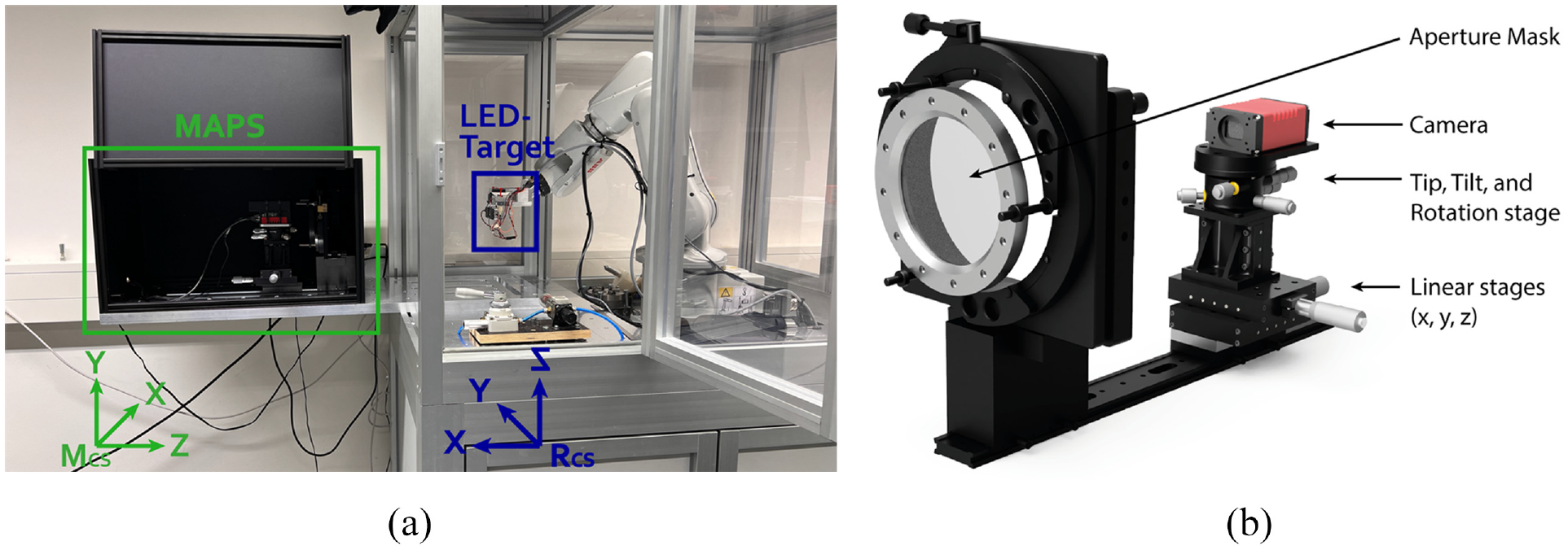
The experimental set-up: (a) the MAPS detector (box on the left), the LED target on the robot tool (holder for attaching the LEDs) and the robot itself on the far right. The coordinate systems of the two machines are also drawn in the picture. In (b) a closer look at the MAPS can be seen. The aperture mask is mounted in front, behind it the camera, which sits on several optical stages to allow the sensor to be adjusted in six degrees of freedom.
The MAPS measuring device consists of a high-resolution camera, an aperture mask mounted in front of the camera and an LED target. 25 The aperture mask is a 1 mm thick glass plate covered with a layer of chrome, into which about 40 k holes are etched. The camera is a Prosilica GT 3300 from Allied Vision with a sensor resolution of 3296 × 2472 pixels at a pixel pitch of 5.5 µm. These two components make up the MAPS detector, which can be seen in Figure 1(b). MAPS is based on the principle of the pinhole camera. The light from the LED target passes through the apertures of the aperture mask and hits the camera sensor. The result is an image with about 800 light spots with a Gaussian-like intensity distribution. By calculating the centres of all these light spots, vectors can be spanned starting at the centres of the light spots, passing through the apertures and intersecting in one point – the position of the light source. With this method, the position of the light source and thus of the robot TCP can be calculated.
MAPS works in a measuring volume of 1 m × 1 m × 1 m with a measuring accuracy of 2.8 µm (2
Methodology
Online correction of a robot TCP can be done in several ways. One is to add a correction value to the current TCP origin so that the robot compensates for its deviation. Another method is to correct all positions in the previously created point list by the correction value and transmit the corrected point list to the robot controller. The latter involves two problems: firstly, the correction value must be applied to all future positions in the path and secondly, the ABB robot controller does not allow the position that is currently being approached to be changed, so that a TCP correction between two positions is not possible. For this reason, the first method is used.
Path planning
The PCAPS software can create simple paths such as lines, meanders, circles and other basic geometries. It is possible to set the dimensions, the spatial position as well as the TCP speed and the density of the point list. PCAPS is also used to create the trajectories that are used to calibrate the MAPS or to move to a specific position. More complex paths are created by computer-aided manufacturing (CAM) or slicer software. They generate GCODE that can be imported by PCAPS. The preprocessor then translates the position and velocity data into robot commands. The path thus created is then broken down into even smaller parts that are transferred one after the other (buffered transfer), so that there is no need to wait until the entire point list has been transferred.
Calibration of MAPS
The MAPS coordinate system
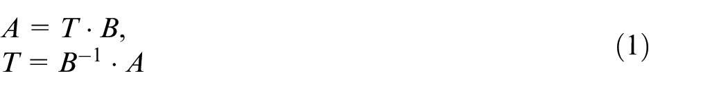
where
Since it is impossible to align both CS perfectly, a combination of two errors occurs during the calibration:
Offset: when there is a translation error between the two systems (origins do not match).
Drift: when there is a rotation error between the two systems (axes not parallel).
Online position correction design
The online position correction (OPC) is a control loop with three main components: the MAPS, the robot with its controller and the OPC algorithms, as shown in Figure 2. As mentioned earlier, the planned path is created on the master computer and transmitted to the robot controller. The same tool path is also known to the position correction algorithms, where it is used to calculate the deviation from the measured TCP position to the planned position. The deviation

where
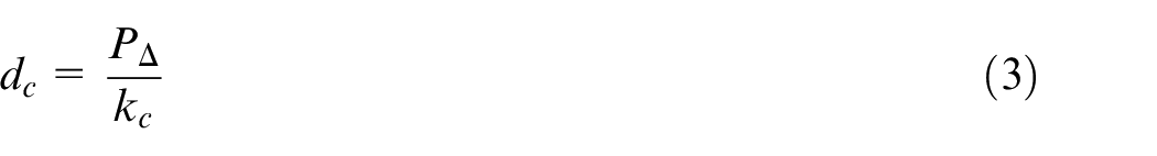
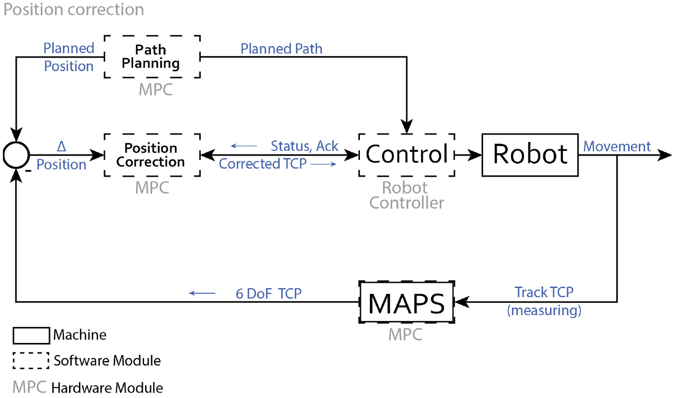
Block diagram of the position correction control loop with the most important software and hardware components. By detecting the current TCP position with MAPS, the correction loop determines the deviation from the originally planned position, from which a corrected TCP position is calculated. This is then transmitted to the robot controller, which shifts the TCP origin accordingly to end the loop.
After that the correction value

The corrected TCP is then sent to the robot controller. While the OPC manipulates the TCP origin position, it causes the robot to move its end effector by the corrected value. This moves the entire planned path and applies the correction to all pending positions.
Experimental results
To evaluate the performance of the OPC, three different experiments were conducted, each with and without OPC. The TCP speed is set to 0.5 mm/s, adapted to the measurement frequency, with a payload of approximately 0.5 kg. MAPS is calibrated on the robot platform to align both the MAPS coordinate system and the robots. The aim of the experiments is as follows:
Testing the path accuracy of the robot on its x-, y- and z-axis by moving the robot end effector along each axis.
Testing the positional accuracy of the robot by moving the end effector several times from different positions to the same starting position.
Testing the z-axis stability of the robot by driving a circular path in X and Y directions with a fixed z-plane.
The results of the aforementioned experiments are discussed in the following section. In the Figures 4 to 6 the results of the linear path experiment are shown as deviation from the planned position, each experiment separately. Both the corrected and uncorrected results are shown. The results of the circular orbit experiment are shown in Figure 7. The graph shows the z-deviation from the planned position over time. Figure 3 shows the results of the position accuracy experiment, again as deviation from the planned position with and without correction in all three axes.
Remark, that the accuracy of the robot shown in the following results cannot be directly compared to the accuracy stated by the manufacturer, as a different speed, as well as a different payload, is used in the experiments.
Position accuracy and correction
To determine the positional accuracy of the uncorrected and corrected robot, an origin position
Drive from the offset position
Take 100 measurements with MAPS.
Drive to the next offset position
Repeat steps 1–3 until the origin is approached from all eight offset positions. Then the experiment is repeated with the online correction, the OPC corrects the robots position after each time approaching the origin position. The experimental results are shown in Figure 3(a). The box plots represent the repeatability in approaching the planned position (
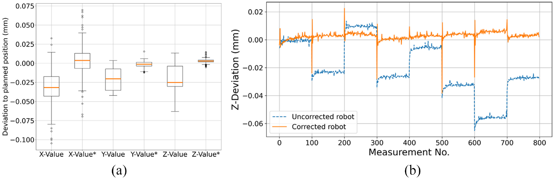
The results of the position accuracy experiment are shown as deviation from the planned positions for all three linear robot axes without and with position correction (marked with *) in (a). The deviation in the z-axis from the planned path in mm against the measurement number is shown in (b). The original position was approached from eight different offset positions. Then 100 measurements were made with MAPS forming a segment shown in (b). This graph also shows that the TCP error depends on the offset position from which the origin position is approached. The OPC improved the MAE deviation by 10 for the x-axis, 13 for the y-axis and 7 for the z-axis.
As can be seen in Figure 3(a), the OPC improved the positional accuracy of the robot, recognisable by the fact that the mean value (solid line in the box) is closer to zero. The mean deviation in the uncorrected experiment is −0.0311 mm for the x-axis, −0.0218 mm for the y-axis and −0.0205 mm for the z-axis, with outliers between −0.75 and 0.1 mm. The corrected mean deviation values are much closer to zero at 0.0032 mm for the x-axis, −0.0017 mm for the y-axis and 0.0029 mm for the z-axis. This is an improvement of about a factor of 10 in x, 13 in y and 7 in z.
The mean deviation values are interpreted as the position accuracy of the robot-MAPS system, while the outliers indicate the maximum error for each axis. The measured values include the MAPS measurement uncertainty and the TCP inaccuracy of the robot. The smaller boxes and whiskers in the plot of the OPC experiment mean that the dispersion of the measured values has decreased. Therefore, the standard deviation has improved by a factor of 1.1 for the x-axis, 3.5 for the y-axis and 9.1 for the z-axis. There are still outliers in the box plots of the corrected system. They occur because the correction only starts when the end effector has reached the original position, that is, the first measured values are not corrected.
An interesting finding is that the accuracy of the robot varies depending on which offset position the origin is approached. This means that the positional accuracy depends on the position of the rotational gears of the robots joints and which ones are used to move the end effector from position
In general, it can be observed that the OPC corrects the errors in all three linear axes, regardless of the offset position from which it was approached. For both y- and z-axis correction, the corrected position is in a range of
Considering that the MAPS was calibrated on the uncorrected robot system, it is important to note here that the measured values may be subject to uncertainties like those of the uncorrected robot in this experiment.
Linear path correction
To test the path accuracy of the robot in this experiment, six trials were conducted. One for each linear axis of the robot, each with and without OPC. The origin position
From there, the end effector of the robot moves 100 mm in the z-axis at a speed of 0.5 mm/s. It should be noted that no correction is currently possible in the direction of travel, as this leads to synchronisation errors. For this reason, only the results for the perpendicular axis are discussed below.
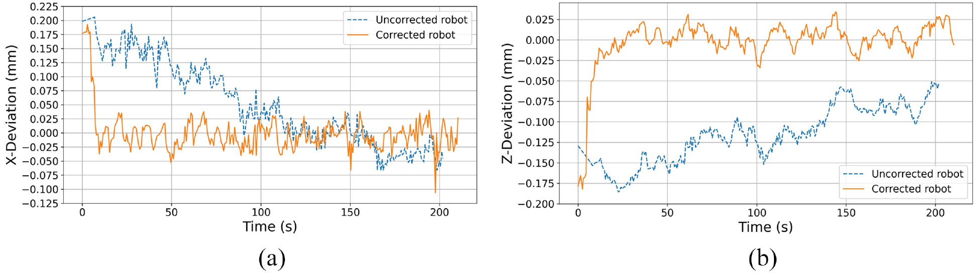
Figure 4 shows the results of the first two trials on the x-axis. In (a) the deviation is plotted on the y-axis, in (b) the deviation on the z-axis. The diagrams with the dashed lines represent the uncorrected robot system, the diagrams with the solid line the corrected robot system. The corrected and uncorrected deviation diagrams in (a) show a similar profile, but in the uncorrected diagram an offset from the beginning can be observed as well as a jump at about
Mean and MAE values in mm for all six trials of the linear path correction experiment, shown for each axis individually.
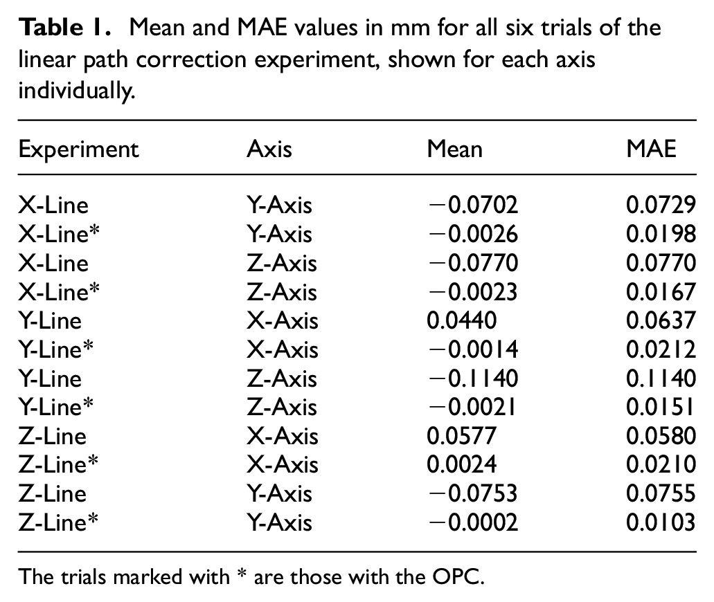
The trials marked with * are those with the OPC.
Linear movement in the x-axis: deviation in the y-axis (a) and in the z-axis (b) from the planned path in mm against the trial time in s. Both trials, uncorrected (dashed line) and corrected (solid line), are shown in the same graph.
The z-deviation of the same trials in Figure 4(b) shows a similar offset at the beginning as well as a drift from the offset to the planned position. The OPC was able to correct both errors, reducing the mean value from −0.0770 mm of the uncorrected system to −0.0023 mm of the corrected system.
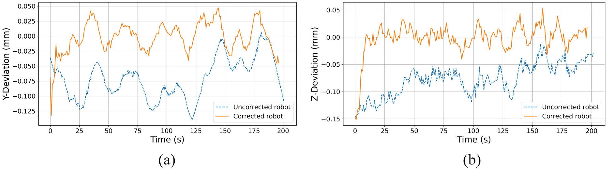
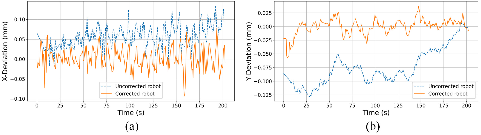
Looking at the x-deviation in the y- and z-axis trials in Figures 5(a) and 6(a), again a drift can be seen. In the y-trial, the TCP drifts away from MAPS (negative slope) and in the z-trial, the TCP drifts towards MAPS (positive slope). This indicates that the drift is robot related. Besides this, no other significant systematic error is observed and the remaining error is considered random due to vibration, load and low stiffness of the robot. The mean value of the x-deviation for the y-axis was improved from 0.0440 to −0.0014 mm and for the z-axis from 0.0577 to 0.0024 mm.
Linear movement in the y-axis: deviation in the x-axis (a) and in the z-axis (b) from the planned path in mm against the trial time in s. Both trials, uncorrected (dashed line) and corrected (solid line), are shown in the same graph.
Linear movement in the z-axis: deviation in the x-axis (a) and in the y-axis (b) from the planned path in mm against the trial time in s. Both trials, uncorrected (dashed line) and corrected (solid line), are shown in the same graph.
Comparing the z-deviation in the x- and y-axis trials, the deviation plots of the uncorrected robot system look very similar. The deviations start at about the same position and the TCP drifts with an almost identical slope in the direction of the planned path in both trials. This suggests that the drift may be due to a calibration error of MAPS and not just the robot itself. The calibration process at the beginning of the trials serves to align the robot axes with the MAPS axes. Since it is impossible to align them exactly parallel to each other, a small error always remains in the calibration. This angle between the MAPS and the robot axes can lead to a measurable drift. Since it was observed earlier that the robot also drifts, the drift error, in this case, can be a combination of both errors. In the diagrams where the OPC has corrected the robot system, the drifts are no longer present because both the robot drift and the calibration error are corrected.
Another artefact can be observed in the uncorrected plots. Besides the general drift, the deviation is constant (except for the random error) in two intervals:
Figure 6(b) shows again that the OPC reliably corrects the low-frequency errors, as they are no longer present in the corrected path. On the other hand, in this experiment it was not possible to correct the high-frequency errors because MAPS currently works with a low measurement frequency (about 4 Hz). Therefore, the correction algorithm also operates at a low frequency, which makes the correction loop somewhat sluggish. This is to be improved in the future by integrating a much faster camera into MAPS. Whether these errors can be corrected at all depends on their origin. It will be very difficult to correct a vibration-related error caused by the low stiffness of the robot, for example. A closer look at Figure 6(a) reveals a strong noise in both lines. This effect is due to the fact that MAPS measures less accurately in the direction of its optical axis z (the x-axis of the robot) than in the other axis directions. 25
As mentioned earlier, the calibration of the MAPS is used to align the robot CS with the MAPS CS. However, a calibration error always remains, which can lead to non-parallelism of the robot and MAPS axes. This in turn leads to a drifting measured value. As a reminder, in the first experiment in which the positional accuracy of the robot was determined, a maximum deviation of 0.105 mm in the x-axis, 0.042 mm in the y-axis and 0.063 mm in the z-axis was measured. Considering that the MAPS was calibrated with this inaccuracy, it is not unreasonable to see a deviation from the planned path in the measured values. The reason for this is that the calibration vectors are defined with several positions that the robot approaches. If the robot does not travel an exact, parallel line to its base system axis, there is an error in the calibration. If a line is then drawn along the linear axis of the robot, it looks as if the robot deviates from its planned path.
From the experimental results, there is a drift in the z-axis associated with the MAPS calibration error and a drift in the x-axis associated with the robot error. For the MAPS-related errors, a combination of the robot position inaccuracy and the MAPS calibration inaccuracy is measured. This means that all measurements are also affected by the errors of both systems. Therefore, a more accurate calibration process is needed to ensure that the measurements do not drift. This can be achieved, for example, by repeating the calibration routine several times at different positions. Calibration of MAPS with a coordinate measuring machine (CMM) is also considered, as the CMM is much more accurate than the robot. Only then can it be said with certainty that the remaining drift is only caused by the robot itself. For the experiments, this means that the improvement in accuracy could be less than the results show, as the error of MAPS is also corrected. Nevertheless, the experiments show that a drift can be corrected regardless of its cause.
Table 1 sums up the results of the trials. The first column shows the 12 trials, the trials marked with an * are with the OPC. The third and fourth columns show the mean and MAE error against the planned path for the axis listed in column two. It can be observed that the correction results of the z-axis in the y-line trial and the y-axis in the z-line trial are better than the results in the x-line trial for the same axis. This means that the OPC is less effective in the MAPS optical axis. This effect can be explained by the operating principle of MAPS. When the light source is moved along the optical axis or parallel to it at a small distance, the angle of the light beam between the aperture mask and the camera sensor changes only slightly compared to a perpendicular movement of the light source. This results in a smaller change of the image, which leads to higher uncertainties on this axis. For this experiment, it can finally be said that the accuracy of the robot with respect to the MAE has improved by a factor of 2.7–7.5, regardless of the source of error.
Circular path correction
A circular path with a diameter of 50 mm (xy plane) at a fixed z-position is planned. This experiment is intended to measure the accuracy with which the robot can hold a fixed z-level while travelling on a 2D path. The experiment includes two trials, one without and one with the OPC. MAPS is again used to measure the TCP position in these trials. The origin position
Figure 7 shows the deviation from the planned path of both experiments as line diagrams. Looking at the uncorrected robot trajectory, an initial offset of about 0.08 mm in the z-axis can be seen. This is the same effect that was explained in the previous experiment. There is no significant drift, but it is also noteworthy that the deviation is again not constant, but depends on the position of the end effector on the circular path. This behaviour was also observed in the position accuracy experiment, which means that a correlation between the TCP accuracy and the position of the robot joints can also be observed here. This leads to a maximum deviation of more than 0.2 mm on the z-axis, a MAE of 0.1196 mm and a mean value of −0.1196 mm.
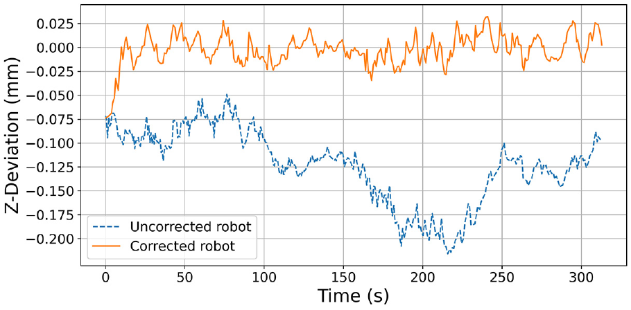
Deviation in the z-axis from the planned trajectory in mm against the trial time in s of the experiment to measure and correct the circular trajectory. Both experiments, the uncorrected (dashed line) and the corrected (solid line), are shown in the same graph. The initial offset and the error measured by MAPS with respect to the TCP position were both corrected by the OPC.
By repeating this experiment with the OPC, an improvement in accuracy (MAE) of about a factor of 10 is achieved (0.0116 mm). The initial offset is also corrected, resulting in a z-deviation of about
Conclusion
With the presented online position correction algorithms and the new MAPS measurement device, it is possible to measure and correct the end effector of an ABB industrial robot in several disciplines. In a first experiment, the comparatively low positional accuracy of the robot was determined. Note that the deviation depends on which axial joints the robot uses to move to the planned position. Through this correction, the accuracy could be improved by a factor of 7–13, depending on the axis. The analysis of the path accuracy leads to the conclusion that there are high and low frequency errors as well as an initial offset and drift in the TCP path along the linear axis. The low-frequency errors, the offset and the drift could be corrected. The path accuracy could be improved by a factor of about 2.5–7.5 again, depending on the axis. The high-frequency errors could not be corrected because of the low measurement frequency. The circular path experiment proved the hypothesis that the z-position of the robot fluctuates in the xy plane while travelling on a 2D path. Again, a correlation was found between the end effector position and the TCP error. The OPC corrected the deviation and increased the accuracy by a factor of 10.
In conclusion, it has been shown that MAPS is able to measure random and systematic errors of the robot, which can be partially corrected with the OPC. The OPC was shown to improve the robots TCP position accuracy and trajectory accuracy many times over, while reducing certain errors such as offsets and drifts. By calibrating the MAPS on the robot, the two coordinate systems were aligned. In this way, and through the operation of the OPC algorithm, the robot is always corrected to the measured TCP value. This is not a problem, but rather an advantage, as long as the work piece coordinate system is also calibrated to the other. So the key to precise tool correction is accurate calibration of the coordinate systems of the robot, the MAPS and the work piece. The experiments carried out do not cover the entire working range of the robot nor its full speed potential and should therefore only be considered as a proof-of-work of the new measuring device MAPS in combination with the OPC. Further experiments need to be conducted to determine the full potential of the system. The results also show that moving the light source on or parallel to the optical axis of the MAPS leads to higher uncertainties in the measurements and thus to a worse correction result. Positioning the MAPS at a certain angle that is not parallel to the robots axis of motion could improve the accuracy of the system.
In future work, the MAPS calibration routine should be improved on the robot or moved to a high-precision machine such as a CMM. This should reduce the error in calibration that leads to measurement drifts. Future research should also investigate the performance of the OPC at higher speeds. This requires using a camera with a higher frame rate so that a sufficient number of readings can be recorded. This not only increases the movement speed of the robot in OPC operation, but also shortens the reaction time of the correction to a measured error. It must then be investigated whether a higher system frequency can be used to correct the higher frequency errors. As mentioned above, this depends on the cause of the error, for example, the mechanical properties of the robot, its stiffness, etc. An analysis of the vibrations and other influencing factors could be done in advance to be sure what kind of errors the OPC is dealing with.
Footnotes
Declaration of conflicting interests
The author(s) declared no potential conflicts of interest with respect to the research, authorship, and/or publication of this article.
Funding
The author(s) disclosed receipt of the following financial support for the research, authorship, and/or publication of this article: This research is funded by the German Federal Ministry for Economic Affairs and Climate Action under the programme of ‘Zentrales Innovationsprogramm Mittelstand’ in short ZIM (OMTS-I 4.0 – OnPoRob with contract no 16KN075728) and by the German Research Foundation short DFG (‘Precise, flexible and modular 6 dimensional additive manufacturing platform including individual in-situ analysis’, contract number BO 3489/1-2). The Author’s would like to thank the German Federal Ministry for Economic Affairs and Energy, the German Research Foundation and eµmetron GmbH for funding this research.