Sage Journals: Discover world-class research

Abstract

Due to the increasingly variable market competition, product modular design is gaining in importance. This study attempts to seek a balance in three perspectives on product design: connection intensity, cost-effectiveness, and environmental protection. A multi-objective grouping genetic algorithm is adopted. Grouping genetic algorithms feature the flexible grouping and correcting mechanisms of crossover and mutation to meet the requirements of grouping, making it possible to establish a reasonable multi-objective measurement method after grouping and further offer suggestions to improve the modular design. In this study, the ceiling fan is used as an example to verify the proposed method for evaluation of the grouping method in the Matlab program. Results of the ceiling fan case verify that the proposed multi-objective algorithm is effective in modular design.

Keywords

Modularization group genetic algorithm recycling value green lifecycle

Introduction

Modularization divides a product into smaller units. After these small units are independently designed, they are integrated into a complex product. In modularization, the module must respond to the role it is assigned in terms of product function, and the way the parts are connected is the most important factor.¹ In addition, modularization involves different perspectives, such as manufacturability, cost, green life cycle, and supply chain. A good modular design can effectively reduce production costs and allow quick combination of the parts into new products to respond to changing demands. Many studies in the past have explored these different issues.^2–5

Modular design is usually described by a network model, and then network partitions are studied to form a separate module (or subassembly). In the past, many researchers have proposed different methods to solve the problem of modularization, such as a triangularization algorithm with a matrix operation,⁶ coupled with Quality Function Deployment and Grouping Genetic Algorithms (GGAs),⁷ similarity analysis,⁸ machine learning-based flexibility analysis,⁹ the assembly planning viewpoint,^10,11 axiomatic design and the design structure matrix (DSM),¹² DSM and improved elbow assessment method.¹³

In the cost-benefit consideration, Zhang and Gershenson¹⁴ focused upon the cost model of the life cycle, and Fujita and Yoshida¹⁵ constructed a cost model and proposed an optimization model for product variety. Tseng et al.¹⁶ established the calculation of cost profit from the disassembly point of view. Agrawal et al.¹⁷ concentrated on the cost-profit model to screen modules under the product family structure. The discussion of cost and profit makes module considerations an important measure of economic perspective.

The life-cycle-oriented modular approach focuses on environmental considerations in product design and the reduction of the impact of the product on the environment after its life span. Newcomb et al.¹⁸ developed green modular design primarily with group techniques. Gu and Sosale¹⁹ considered the connection, assembly, service, and reuse/remanufacturing/recycling factors among components in the design phase, and they used the Simulated Annealing algorithm to explore modularization. Tseng et al.²⁰ defined connection intensity from the so-called Connection Graph and adopted GGAs for green and cost considerations. Smith and Yen²¹ used atomic theory to explore modularization by taking the factors of material compatibility, recyclability, and disassemblability into consideration. Yu et al.²² continued with Kreng and Lee’s idea, extending it to economic and environmental considerations. Yan and Feng²³ adopted the so-called 6R (reuse, recycle, reduce function, manufacturability, and end-of-life) and the DSM to solve the modularization problem so as to reduce the burden on the environment.

In recent years, some researchers have also taken a comprehensive multiple perspective to explore the modular problem. For example, Ameli et al.²⁴ focused on the balance between life cycle and cost to establish an optimal model. Yang et al.²⁵ proposed a multi-objective green modularization method based on risk control, from which three objectives, namely, reuse, maintenance, and recycling, were expressed in the fitness function, and then they used GGAs to explore modularization. Most of the above-mentioned studies turned multiple objectives into a single goal to explore modularization. You and Smith²⁶ used atomic theory and a fuzzy c-mean approach to integrate functional and environmental protection. It is proposed that each group of modules should be highly independent and unique.

The discussion of single targets based on GGAs has yielded some results in past research.²⁰ To meet the changing needs of today’s complex environment, this study intends to expand GGAs to multi-objective grouping genetic algorithms (MOGGAs) for the evaluation of modular design. This study adopts the concept of 3R1T in the green life cycle design. 3R1T refers to four recycling strategies of Throw Away, Re-Cycle, Re-Manufacture, and Re-Use. The parts are recycled mainly by using these four strategies. Secondly, the authors establish a cost-effective measurement method to check the recovery value of the parts and then adopt the connection intensity method to explore the connection strength of the product modules.

As far as the synchronous integration of recycling strategies is concerned, due to the restraint between the objectives and the difference in the units between the objectives, the influence of each objective on the overall objective function is different. Therefore, it is difficult to measure the overall performance. Since such problems are not easily solved by single-objective planning, this study adopts the multi-objective Pareto optimization solution method. Each target value is given, and optimization of each target is performed at the same time. The number of Pareto optimal solutions generated at the end is usually not unique, so it can provide users with more flexible solution choices. In the past related studies^27,28 comparing MOGGAs with other algorithms, the results showed that MOGGAs have better test performance in terms of quality or quantity of Pareto optimal solutions. Therefore, in the multi-objective design, this study adopts the MOGGA architecture. It is hoped that the MOGGA methodology will be comprehensive due to the consideration of multiple perspectives in product modular design.

Methodology

Assumption and procedure in MOGGAs

The basic assumptions listed in this study are as follows:

(1) Only the manual assembly operations are suitable, and robotic operation is not applicable.

(2) The direction of accessibility is limited to the principal directions of x, y, and z.

(3) The attribute score of connection intensity is assumed to be known and fixed.

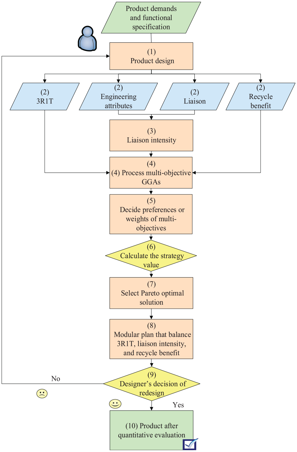
In addition, the modular planning method proposed in this study is divided into nine steps, as shown in Figure 1. The steps are described as follows:

Step 1: The designer checks the product requirements and functional specifications for product design.

Step 2: List 3R1T (further discussed in Section 2.2.1), four product engineering attributes (discussed in 2.2.2), Connection Graph, recycling benefits, etc., which will be explained in 2.2.3.

Step 3: Based on four product engineering attributes and the Connection Graph, establish the connection intensity between parts.

Step 4: Find the three-objective solutions from the GGA algorithm (Sections 2.3.1 and 2.3.2).

Step 5: The designer determines the degrees of preference of three objectives according to the needs (Section 2.3.3).

Step 6: Calculate the estimated values by using the Pareto optimal solution set and preference level (Section 2.3.3).

Step 7: Find the preferred solution from the Pareto optimal solution set (Section 2.3.3).

Step 8: Perform the modular plan that balances 3R1T, connection intensity, and recycling benefit.

Step 9: The designer decides whether to redesign the product or not. The modification and review of modular design will be discussed in Section 3.2.

Figure 1.

Research flowchart.

Multi-objectives for modular design

3R1T

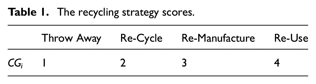
3R1T refers to the four recycling strategies of Throw Away, Re-Cycle, Re-Manufacture, and Re-Use. Throw Away means directly discarding parts without recycling revenue. Re-Cycle refers to restoring the parts to the original materials through special treatment and then re-manufacturing them into new parts for new products. Re-Manufacture refers to reusing the parts in the next product cycle after repair or processing. Re-Use represents disassembling the parts and reusing them directly in the next product cycle. The corresponding scores are given in Table 1, and the recovery strategy score of part i is expressed as CGi. First, discarding is the least desirable recycling strategy, setting CGi = 1, and the other three recycling strategies are given according to the complexity of the processing procedure. For Re-Cycle, CGi = 2; for Re-Manufacture, CGi = 3; and finally, for Re-Use, CGi = 4. Assuming that the recycling strategy for Part i is Re-Cycle, then from Table 1, it is known that CGi = 2.

Table 1.

The recycling strategy scores.

	Throw Away	Re-Cycle	Re-Manufacture	Re-Use
CG_i	1	2	3	4

Connection intensity

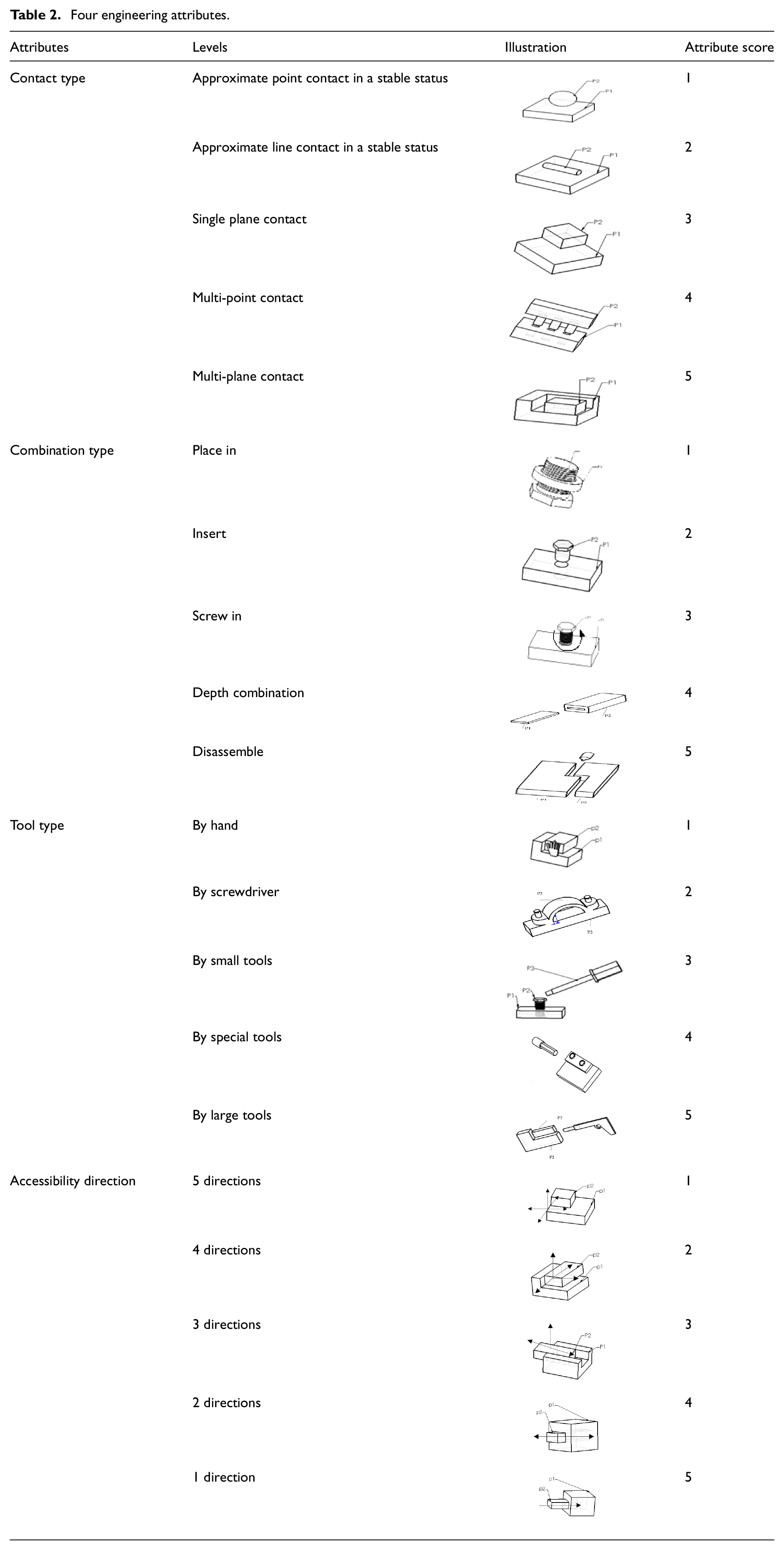
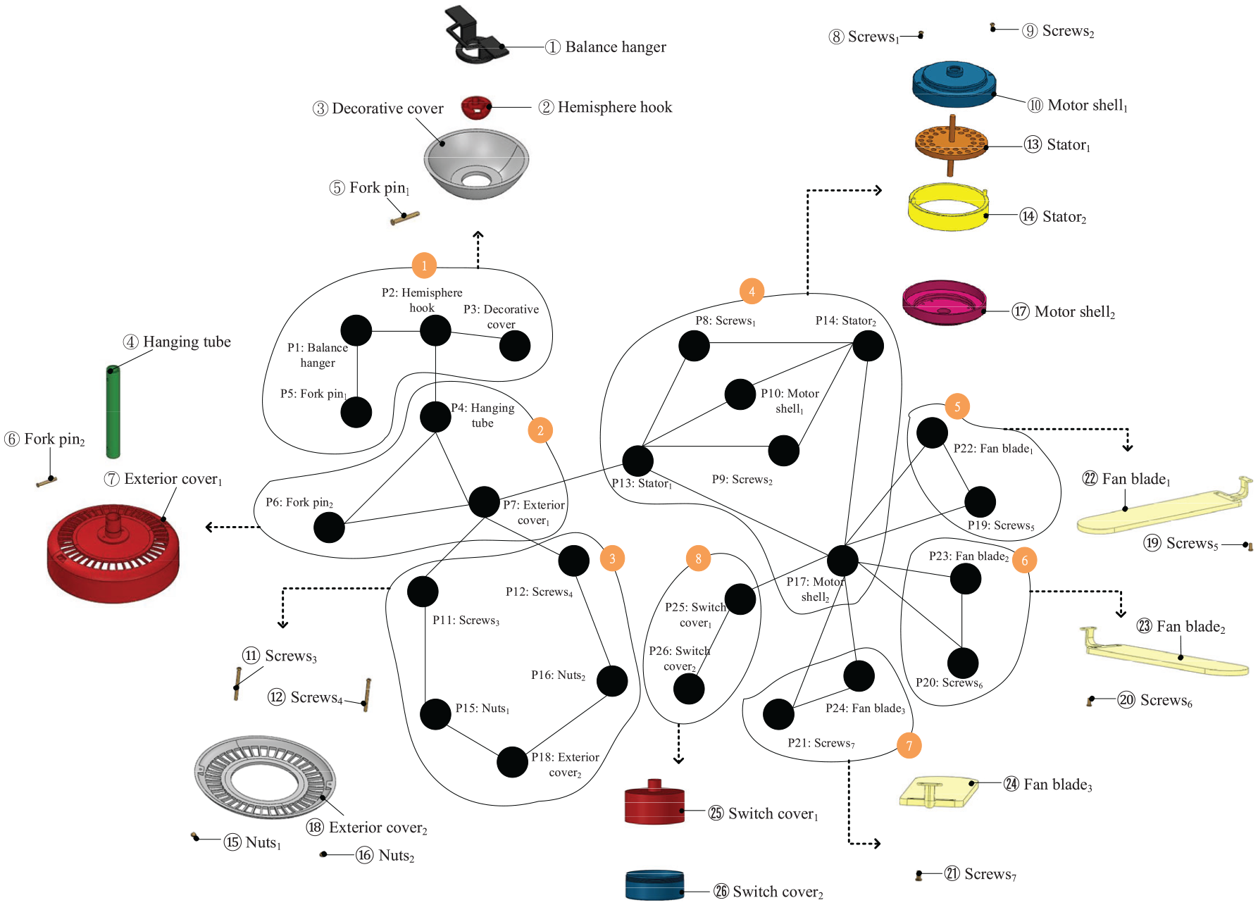
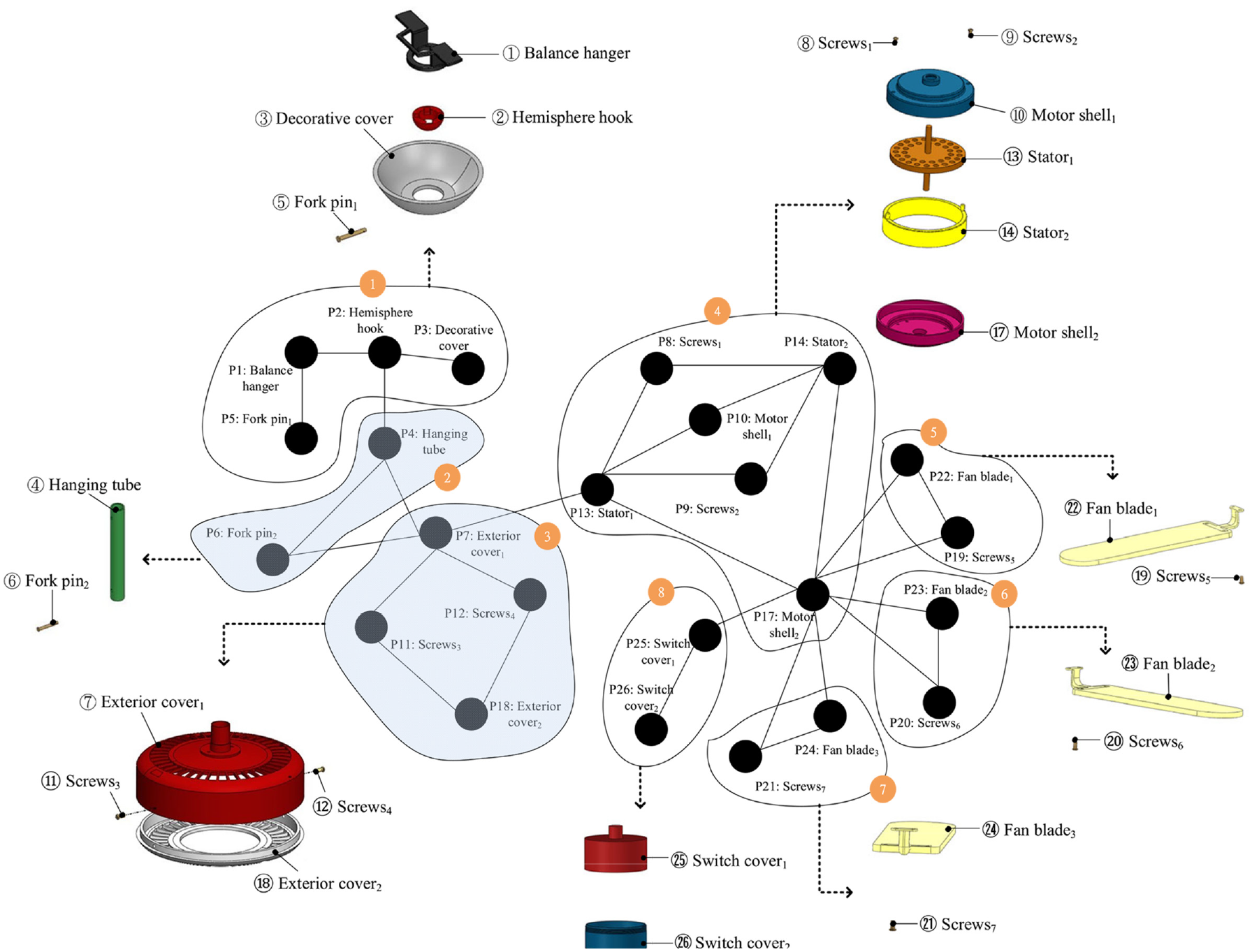
In this study, the ceiling fan of Figure 2(a) is employed as an example. There are 26 parts. The connections between product parts are expressed by the Connection Graph, where one node represents one part and a line describes an engineering relationship between two parts, as shown in Figure 2(b). Four engineering attributes of these parts, namely, Contact Type (CT), Combination Type (CB), Tool Type (TL), and Accessibility Direction (AD), are combined to comprehensively evaluate the connection intensity between parts.^16,29,30 In this study, each attribute is divided into five levels according to the difficulty level, where 1 is easy and 5 is difficult, as shown in Table 2. The connection intensity between parts is determined by the summation of the above four engineering attributes, as shown in equation (1). In the connection between Part 1 and Part 5, for example, the contact type is approximate point contact in a stable state, so 1 point is given; the combination type is depth combination, 4 points; the tool is the hand, 1 point. In terms of accessibility, the parts can be disassembled only from one angle, 5 points. Thus, the total connection intensity of CCS₁₋₅ is 11 points. The connection intensity scores for the parts of the ceiling fan are shown in Appendix A.

CC S_{i - j} = C T_{i - j} + C B_{i - j} + T L_{i - j} + A D_{i - j}

(1)

where:

i: the current Part No.

j: the Part No. after Part i

CCS_i−j: the connection intensity between Part i and Part j

CT_i−j: the contact type score between Part i and Part j

CB_i−j: the combination type score between Part i and Part j

TL_i−j: the tool type score between Part i and Part j

AD_i−j: the accessibility direction score between Part i and Part j

Figure 2.

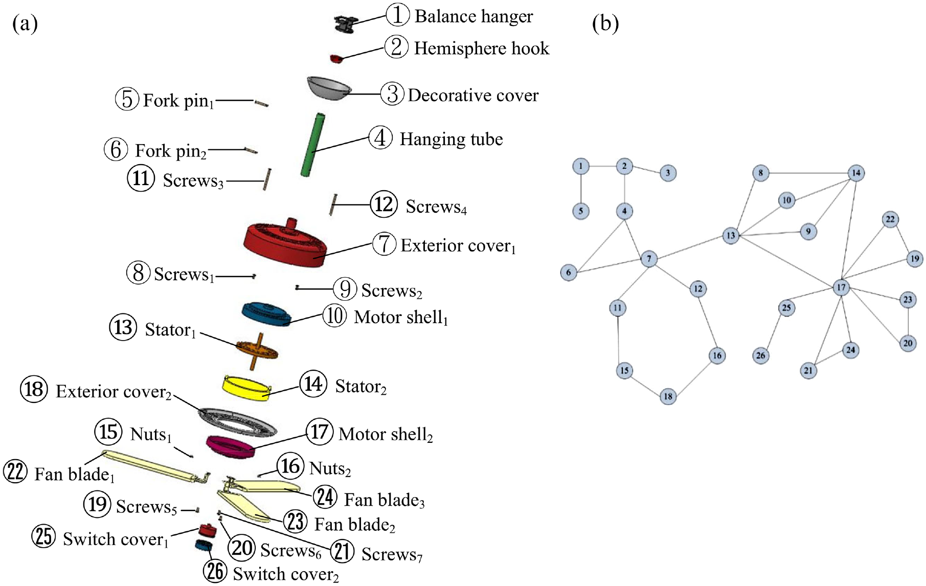
Ceiling fan (a) 3D diagram (b) connection graph.

Table 2.

Four engineering attributes.

Attributes	Levels	Attribute score
Contact type	Approximate point contact in a stable status	1
	Approximate line contact in a stable status	2
	Single plane contact	3
	Multi-point contact	4
	Multi-plane contact	5
Combination type	Place in	1
	Insert	2
	Screw in	3
	Depth combination	4
	Disassemble	5
Tool type	By hand	1
	By screwdriver	2
	By small tools	3
	By special tools	4
	By large tools	5
Accessibility direction	5 directions	1
	4 directions	2
	3 directions	3
	2 directions	4
	1 direction	5

Recycle benefits

Recycle benefits can be calculated based on the recycling strategy of the parts. First, the benefit of Throw Away is set to 0, as shown in equation (2). The Re-Cycle benefit calculation is shown in equation (3). The benefit calculation for Re-Use is shown in equation (4). In this study, the Declining Balance Method (DB) is used to determine the depreciation rate of the product, as shown in equation (5). Finally, the benefit equation for re-manufacture is shown in equation (4). The recycle benefit units calculated by the above equation are converted at the US dollar exchange rate. The recycling benefits of the ceiling fan are shown in Appendix B.

R V_{j} = 0

(2)

R V_{j} = r_{j} \times w_{j}

(3)

R V_{j} = D \times V_{p}

(4)

D = 2 / Y

(5)

where:

j: the current Part No.

RV_j: the recycle benefit of Part j

r_j: the recycle price of Part j from the resource recycle dealer

w_j: the weight of Part j

D: the product depreciation rate

V_p: the price offered by the recycle dealer

Y: product life span

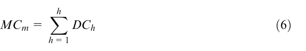
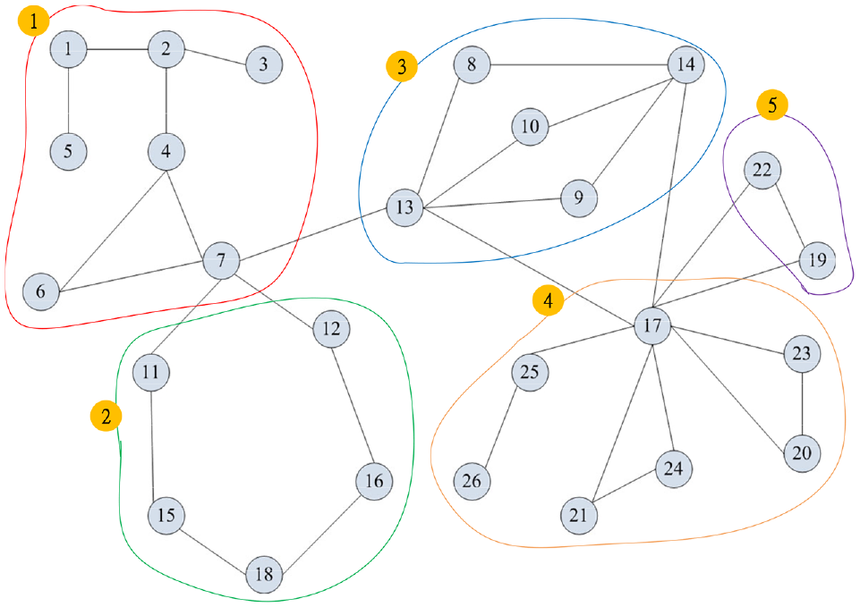
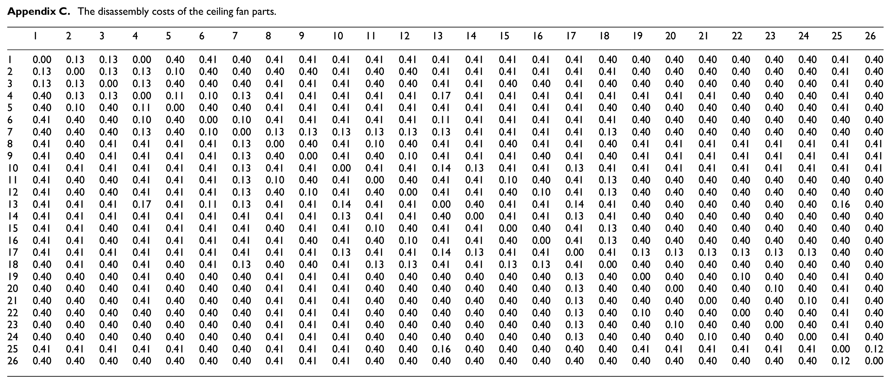
In this study, the module cost (MC) is calculated by equation (6). The decomposition of Module m requires a total of h bond relationships, and DC_h represents the cost of the h bond relationship (in US dollars). Calculate the cost of the bond relationship between every two parts. The cost of the bond relationship for parts of the ceiling fan example is shown in Appendix C. Assume Figure 3 is one of the clustering results of the ceiling fan. For Module 8, a total of two bonds are needed to completely decompose Module 8. That is, the bond relationships are L_17,25 and L_25,26. The costs of bond relationships for L_17,25 and L_25,26 are 0.4 and 0.12, respectively. Therefore, the module cost of Module 8 is 0.40 + 0.12 = 0.52, and the cost of the module is calculated as follows:

M C_{m} = \sum_{h = 1}^{h} D C_{h}

(6)

where:

m: module No.

MC_m: module cost for Module m

DC_h: cost of the h bond relationship

h: number of bonds

Figure 3.

The sample modules of the ceiling fan.

Multi-objective grouping genetic algorithms (GGAs)

Encoding and initial solution to GGAs

GGAs solve clustering problems through exclusive coding (Encoding) and specific Crossover and Mutation mechanisms.²⁴ In the coding of GGAs, a gene represents a module. Take the ceiling fan in Figure 4 as an example. The chromosome of the ceiling fan parts indicates that there are five modules, ABCDE, and the internal numerals represent the included parts.

Figure 4.

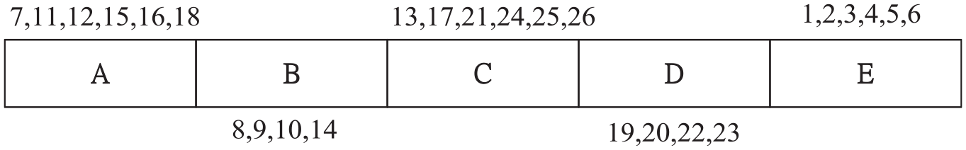
The coding in GGAs.

Suppose Product P is made up of N_c parts, namely, P = {C_j|j = 1,2,…N_c}; that Product P can be divided into m modules; and M_m is the current module number m. The product structure can be expressed as follows:

Product = {M_{m} | i = 1, 2, 3 \dots . m}

(7)

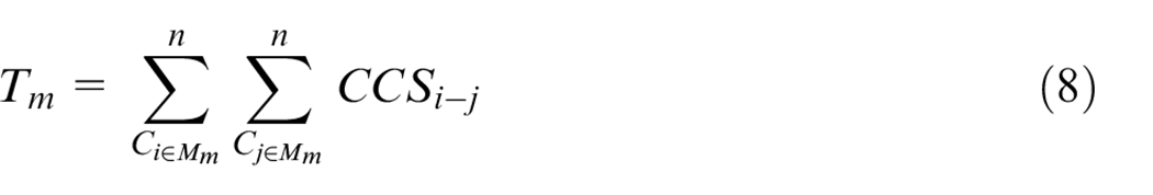
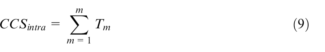
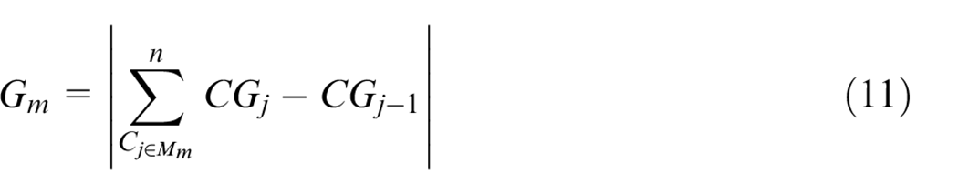
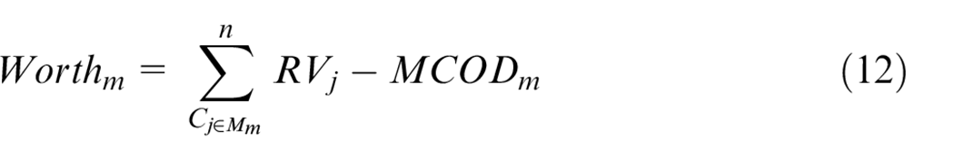
First, the connection intensity is discussed. The connection intensity of Parts C_i and C_j can be expressed as CCS_i−j. T_m represents the sum of the connection intensity scores of all parts in Module M_m. The maximum T_m is obtained. When the connection intensity of the module, CCS_intra, is larger, it is more difficult to disassemble the module. Conversely, a smaller connection intensity CCS_inter between modules indicates that it is easier to assemble and disassemble the modules, as shown in equations (9) and (10). Second, in terms of 3R1T, the 3R1T scores of Cj’s parts can be expressed as CG_j. CG_j−CG_j−1 indicates the difference of the recovery strategy scores between two related parts, and G_m represents the sum of 3R1T scores of all parts in Module M_m. A larger G_m indicates a greater difference in the complexity of the processing strategy of the parts in Module M_m, and vice versa. Therefore, the minimum G_m is the main target. Finally, the recycling benefits can be calculated by equation (12). Worth_m represents the benefit of the recovery strategy minus the cost of the module in the recycling process. The purpose is mainly to maximize the Worth_m. Take Module 8 in Figure 3 as an example. Module 8 (M₈) has two parts, Part 25 (C₂₅) and Part 26 (C₂₆), and the connection intensity between C₂₅ and C₂₆ is CCS₂₅₋₂₆ = 10, so T₈ = 10. The recycling strategy of C₂₅ belongs to Re-Use, CG₂₅ = 4; the recovery strategy of C₂₆ is Re-Use, CG₂₆ = 4; and there is a correlation line between C₂₅ and C₂₆, so CG₂₅−CG₂₆ = 0. Because there are only two parts, G₈ = 0; RV₂₅ = 0.0833; RV₂₆ = 0.0833; MC₈ = 0.52. Finally Worth₄ = (RV₂₅ + RV₂₆)−(MC₈) = −0.3534. Equations (8), (11), and (12) show the equations for the calculation of three objectives.

T_{m} = \sum_{C_{i \in M_{m}}}^{n} \sum_{C_{j \in M_{m}}}^{n} CC S_{i - j}

(8)

CC S_{intra} = \sum_{m = 1}^{m} T_{m}

(9)

CC S_{inter} = CC S_{total} - CC S_{intra}

(10)

G_{m} = | \sum_{C_{j \in M_{m}}}^{n} C G_{j} - C G_{j - 1} |

(11)

Wort h_{m} = \sum_{C_{j \in M_{m}}}^{n} R V_{j} - MCO D_{m}

(12)

where:

m: the current module number

T_m: the connection intensity score of M_m

i: the current part No.

j: the current part No.

n: the number of parts in M_m

M_m: the current module

C_i: the current part is Part i

C_j: the current part is Part j

CCS_i−j: the connection intensity score between Part i and Part j

CCS_intra: the sum of the connection intensity scores of parts in each module

CCS_inter: the sum of the connection intensity scores of parts out of each module

CCS_total: the total of the connection intensity scores of the product

G_m: the 3R1T score of M_m

CG_j: the 3R1T score of Part j

Worth_m: the recycle benefit of M_m

RV_j: the recycle benefit of Part j

MC_m: the recycle cost of M_m

The initial solution of the group gene algorithm is expected to generate diverse and better chromosomes by the following random search:

Step 1: Randomly determine the number of modules in a product.

Step 2: Generate the first part of each module in a random manner.

Step 3: For the remaining parts that have not been grouped, randomly insert them into the parts with the bond relationship in the connection graph. If there is no suitable module, a new module is generated.

Crossover and mutation mechanisms

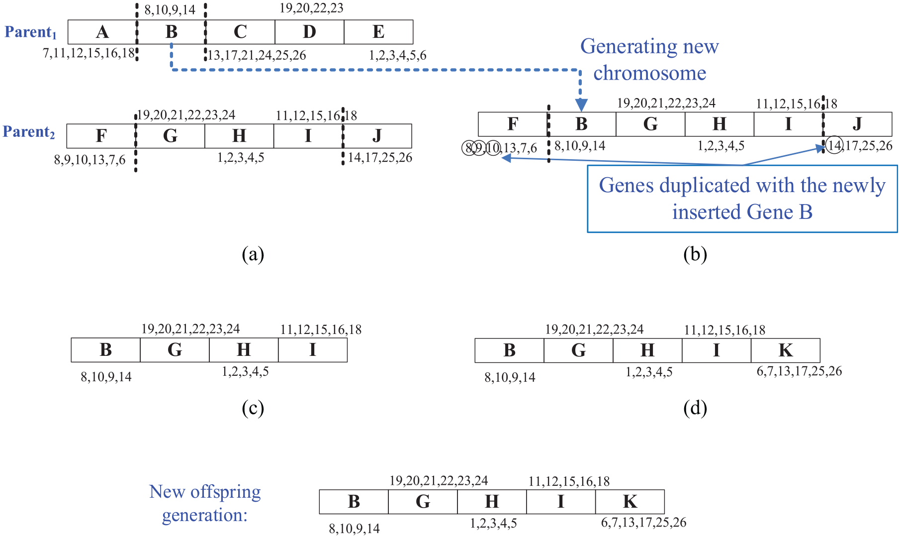
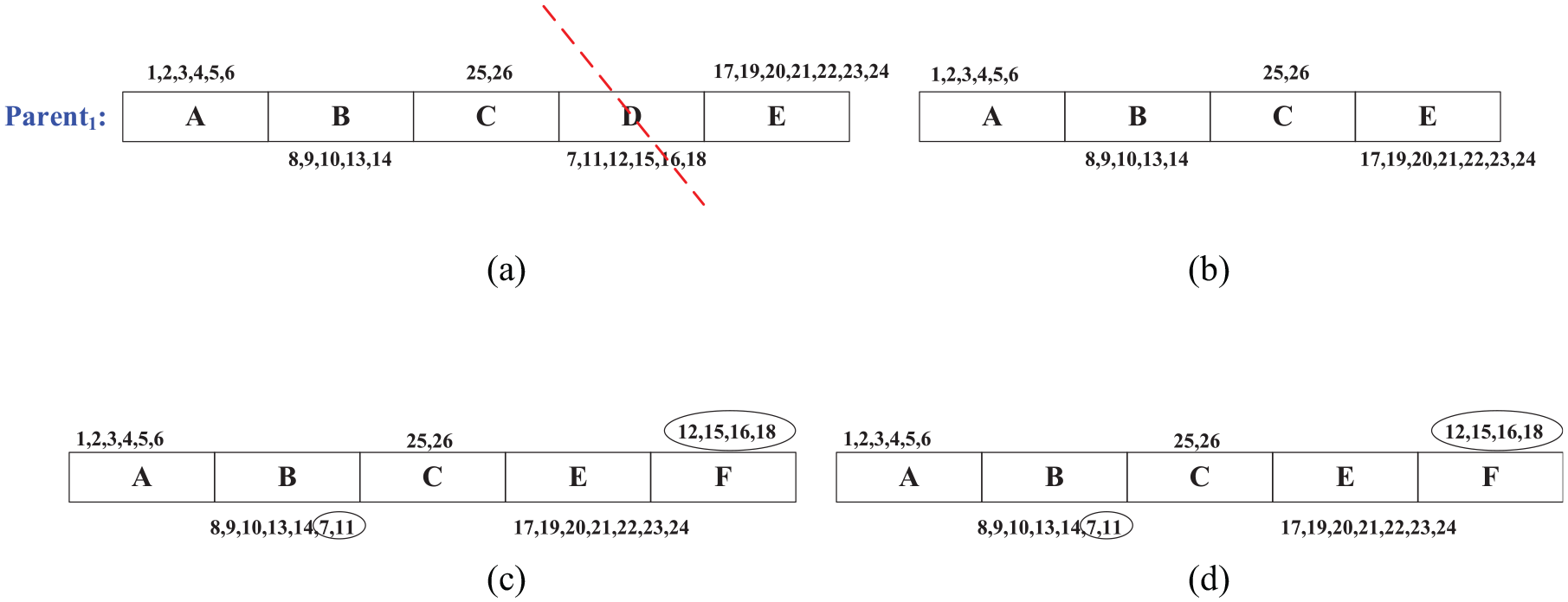
Through constant crossover mechanisms, GGAs generate new generations. In a random manner, crossover points are selected in father and mother generations. Then the crossover segment in the father chromosome is inserted into the crossover segment in the mother chromosome to generate a new child. Moreover, we need to check if there are repeated parts in the new generation. If so, the gene is deleted and the parts of the product missing due to the deletion of the gene are filled in. The above steps are repeated to get another new child. The ceiling fan is used as an example to illustrate the following eight steps:

Step 1: After selecting a pair of chromosomes, randomly generate two crossover points for the crossover segments in each of these two chromosomes. As shown in Figure 5(a), the dotted lines are the exchanged segments of the parent chromosomes.

Step 2: Insert the gene of the crossover segment of the father into the crossover segment of the mother to produce a new chromosome, as shown in Figure 5(b).

Step 3: In the new chromosome, compare whether there are duplicate parts in other genes based on the newly inserted gene, and if so, delete the gene; otherwise, the gene is retained. In Figure 5(b), two modules, gene F and gene J, are deleted. The parts remaining after this deletion are shown in Figure 5(c).

Step 4: Some parts (Parts 6, 7, 13, 17, 25, 26) will be lost due to deletion of the gene, and these parts must be reinserted into the chromosome. Within the limit of the maximum number of parts, insert the missing parts or add them to the module to produce a reasonable and complete chromosome.

Step 5: Randomly select the missing part and check whether the part has a bonding relationship to each part of the gene. If so, insert the gene, and if there are multiple genes that have a bond relationship to the missing part, insert one randomly. If the existing gene has no binding relationship to the missing part, a new gene is randomly inserted or generated. If the existing genes have already reached the maximum number of parts in the module, then new genes can be added. As shown in Figure 5(d), each gene can hold up to six parts. Because genes B, G, H, and I are all full, gene K is added.

Step 6: Check if all missing parts have been reinserted into the chromosome. If yes, go to Step 8; otherwise, go back to Step 5.

Step 7: Calculate the 3R1T, connection intensity and recycle benefit of the module. After Step 3, the new fitness function values of the module (equations (8), (11), and (12)) need to be recalculated.

Step 8: Repeat Steps 2 through 7 for the second chromosome.

In this study, a mutation method is performed to eliminate an already existing group. The genes in the chromosome are randomly deleted, and the missing parts are inserted into the module with the relationships among the parts randomized. It is assumed that if there is no suitable module, a new module will be generated. The ceiling fan is used as an example to illustrate the mutation procedure.

Step 1: Randomly delete any gene in the chromosome as shown in Figure 6(a). The result of the deletion is shown in Figure 6(b).

Step 2: Re-insert the part contained in the deleted gene into the chromosome to make it a complete chromosome, as shown in Figure 6(c). From the missing parts, randomly select a part to check whether the missing part has a bonding relationship to each part of the gene. If so, insert the gene, and if there are multiple genes that have bonding relationships to the missing part, insert one of them randomly. If the existing gene has no binding relationship to the missing part, a new gene is randomly inserted or generated.

Step 3: Check if all missing parts have been reinserted into the chromosome. If not, go to Step 2.

Step 4: Calculate the 3R1T, connection intensity and recycle benefit of the module. Recalculate the fitness function values of the chromosome after mutation (equations (8), (11), and (12)).

Figure 5.

The crossover mechanism in GGAs: (a) select crossover segments, (b) insert the module, (c) the chromosome after deletion of the same genes (modules), and (d) reinsert the missing parts.

Figure 6.

The mutation mechanism in GGAs: (a) select mutation module, (b) delete the module, (c) reinsert the missing part, and (d) new chromosome in child generation.

The Pareto optimal solution set

In this study, the Pareto method is used to search for optimal solutions to the three objectives. Target one is the connection intensity function value, target two is the 3R1T function value, and target three is the recycle benefit function value. These three targets are sought to satisfy the three-objective solution set at the same time. For this reason, they are called Pareto optimal solutions or non-dominated solutions.

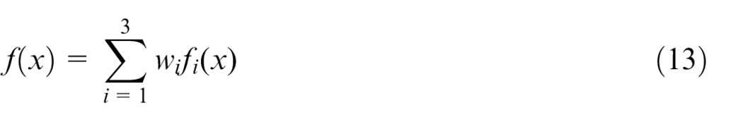
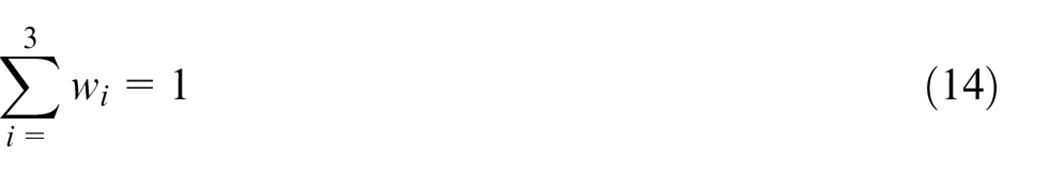
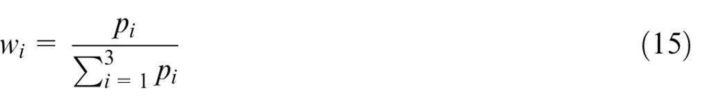
The fitness function of this study is shown in equation (13). This function is a linear combination of the objective function and the weights w₁, w₂, and w₃, which are the non-negative importance of the three targets and satisfy the following relationship in equation (14). The weight value w_i is determined by equation (15), where p_i is a non-negative random real number or a random integer. The change in the weight value can change the search direction to find several different Pareto optimal solutions. These best solutions form the Pareto optimal solution set.

f (x) = \sum_{i = 1}^{3} w_{i} f_{i} (x)

(13)

\sum_{i =}^{3} w_{i} = 1

(14)

w_{i} = \frac{p_{i}}{\sum_{i = 1}^{3} p_{i}}

(15)

where:

f(x): the fitness function

i: number of target

w_i: the weight of target i

f_i(x): the fitness function value of target i

p_i: a non-negative random real number or a random integer of target i

If there are 180 solutions obtained by the Pareto optimal solution set, the solutions are numbered 1–180, and each represents an alternative. For example, alternative 1 is solution No. 1 in the solution set. After the Pareto optimal solution is obtained, the designer can define the preference of each target according to the demand of the product and set a preference degree of 0–1. This method can provide more flexibility for the designer to select alternatives. With the preferences of the decision makers for each goal, the estimated value $f^{i}$ of each target in the decision maker’s mind can be calculated, as shown in equation (16).

f^{i} = f_{\min}^{i} + (1 - p_{i}) \times (f_{\max}^{i} - f_{\min}^{i})

(16)

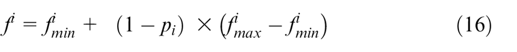
where:

i: number of target

$f^{i}$ : the estimated value of target i

$f_{\min}^{i}$ : the minimum value of target i in the solution set

$f_{\max}^{i}$ : the maximum value of target i in the solution set

p_i: decision maker’s preference to target i

Then we need to calculate the relative distance of each preferred alternative in the Pareto optimal solution set, d_s; the preferred alternative whose d_s is the smallest will be chosen from the optimal solution set, as shown in equation (17).

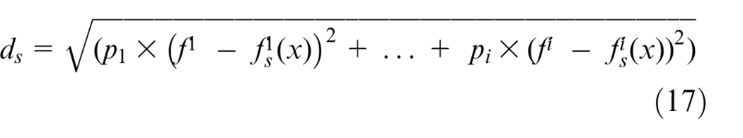
d_{s} = \sqrt{(p_{1} \times {(f^{1} - f_{s}^{1} (x))}^{2} + \dots + p_{i} \times {(f^{i} - f_{s}^{i} (x))}^{2})}

(17)

where:

s: number of alternatives in the solution set

d_s: the distance from alternative s to the estimated value

i: number of target

$f^{i}$ : the estimated value of target i

$f_{s}^{i} (x)$ : the value of target i in alternative s

The user interface

This study uses the preference selection and Pareto’s optimal solution set to establish a graphical operation interface, as shown in Figure 7. This makes it easier for users to input their preferred alternatives and then set up their preferences step by step with the system interface. For preference set up, there are three drop-down menus for targets in the upper part of the interface, and users can choose the degrees of preferences they want. Then they can just click the Start button on the white background to view the preferred result. It is convenient for users to check the details of the alternatives.

Figure 7.

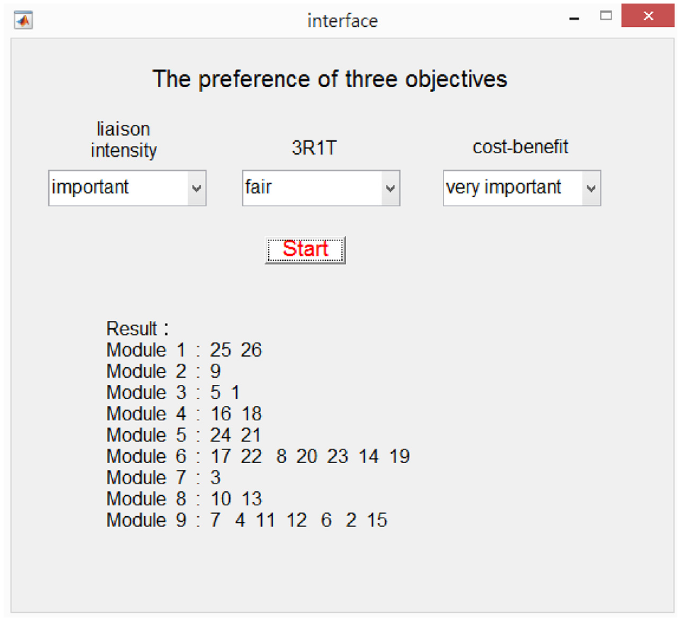
The user interface for setting preferences in multiple objectives.

Simulation testing

Test results and analysis

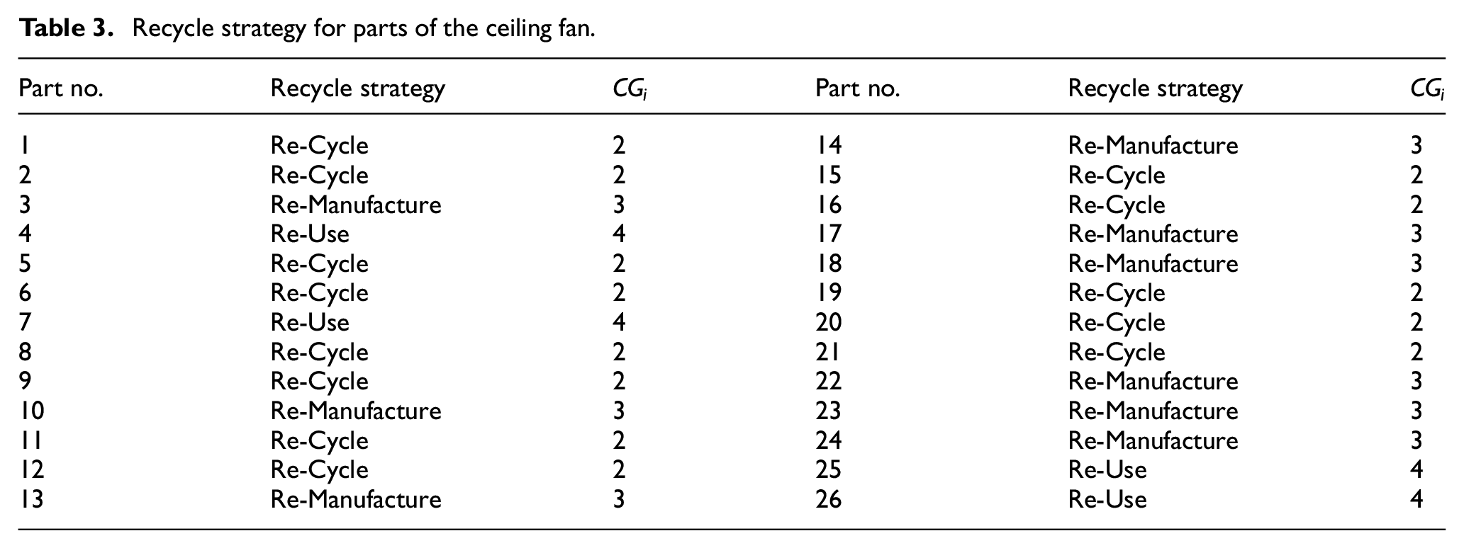
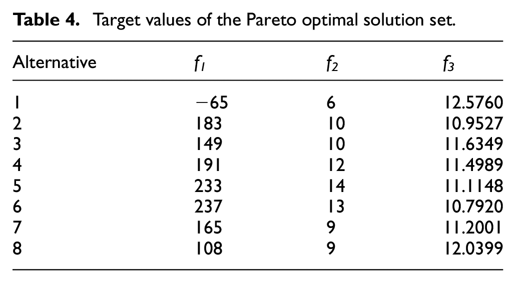
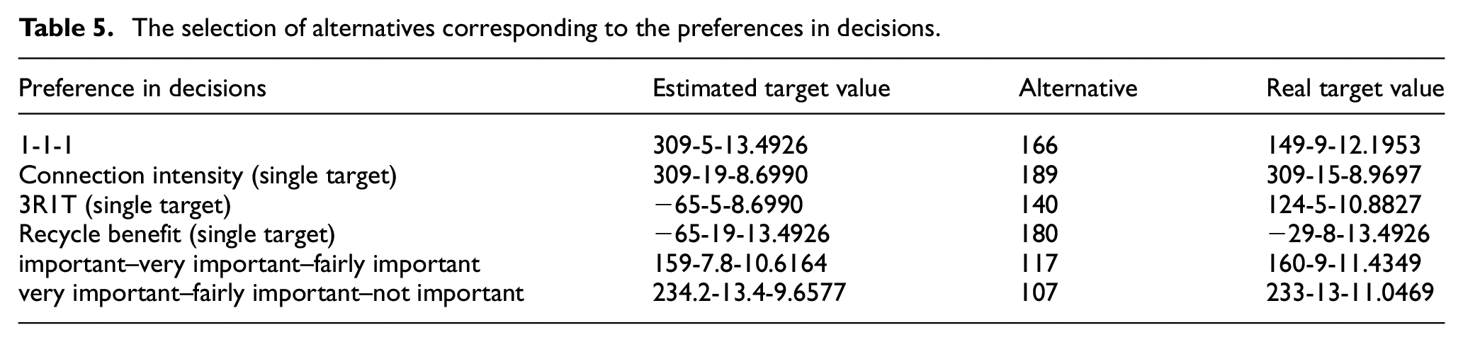
In this study, the programs were written in MATLAB R2015b running in an Intel(R) Core(TM) i5-7200U CPU @ 2.50 GHz 2.71 GHz and 8 GB RAM environment. The recycle strategy scores for the ceiling fan parts are shown in Table 3. The obtained Pareto optimal solution set for the ceiling fan sample case is shown in Table 4. The Pareto optimal solution set can form a plane, as shown in Figure 8, in which no solutions can dominate any other ones. From the optimal solution set, the decision maker can find the desired preferred alternative. In addition, different estimated target values will be calculated from different degrees of preference, as shown in Table 5.

Table 3.

Recycle strategy for parts of the ceiling fan.

Part no.	Recycle strategy	$C G_{i}$	Part no.	Recycle strategy	$C G_{i}$
1	Re-Cycle	2	14	Re-Manufacture	3
2	Re-Cycle	2	15	Re-Cycle	2
3	Re-Manufacture	3	16	Re-Cycle	2
4	Re-Use	4	17	Re-Manufacture	3
5	Re-Cycle	2	18	Re-Manufacture	3
6	Re-Cycle	2	19	Re-Cycle	2
7	Re-Use	4	20	Re-Cycle	2
8	Re-Cycle	2	21	Re-Cycle	2
9	Re-Cycle	2	22	Re-Manufacture	3
10	Re-Manufacture	3	23	Re-Manufacture	3
11	Re-Cycle	2	24	Re-Manufacture	3
12	Re-Cycle	2	25	Re-Use	4
13	Re-Manufacture	3	26	Re-Use	4

Table 4.

Target values of the Pareto optimal solution set.

Alternative	f₁	f₂	f₃
1	−65	6	12.5760
2	183	10	10.9527
3	149	10	11.6349
4	191	12	11.4989
5	233	14	11.1148
6	237	13	10.7920
7	165	9	11.2001
8	108	9	12.0399

Figure 8.

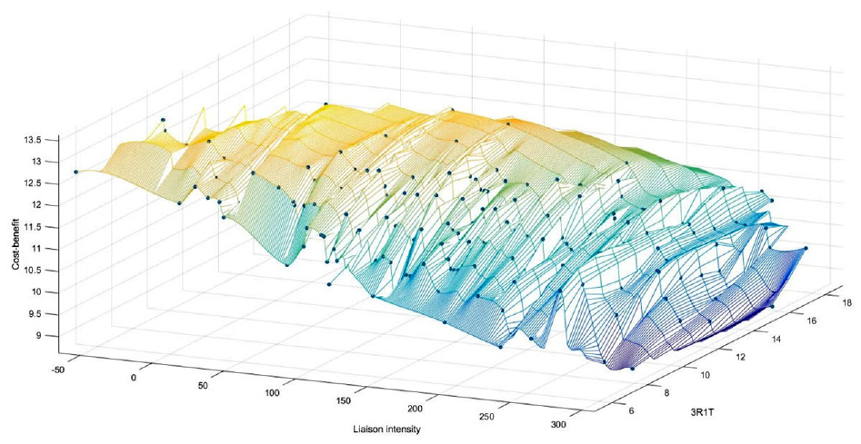
The surface graph of the Pareto optimal solutions.

Table 5.

The selection of alternatives corresponding to the preferences in decisions.

Preference in decisions	Estimated target value	Alternative	Real target value
1-1-1	309-5-13.4926	166	149-9-12.1953
Connection intensity (single target)	309-19-8.6990	189	309-15-8.9697
3R1T (single target)	−65-5-8.6990	140	124-5-10.8827
Recycle benefit (single target)	−65-19-13.4926	180	−29-8-13.4926
important–very important–fairly important	159-7.8-10.6164	117	160-9-11.4349
very important–fairly important–not important	234.2-13.4-9.6577	107	233-13-11.0469

Discussion and modification

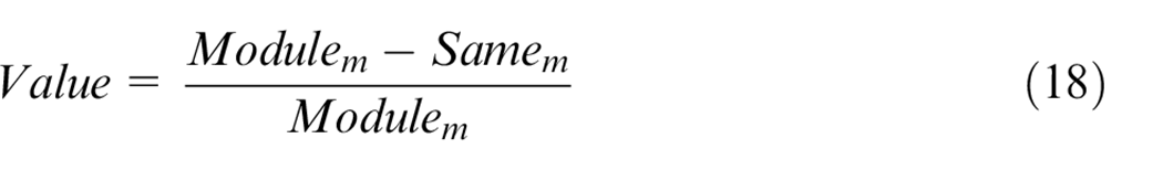
This study employs equation (18) to evaluate the grouping efficiency of the Recycle strategy of each group in the module. A larger value indicates that the recycling strategy in the module is diverse and that there is more room for improvement. In contrast, when a value is smaller, it means that the recycling strategy in the module tends to be the same, and less room for improvement is available.

Value = \frac{Modul e_{m} - Sam e_{m}}{Modul e_{m}}

(18)

where:

m: the current module number

Module_m: number of parts in Module m

Same_m: the number of parts with the most dominant type of recycle strategy in Module m

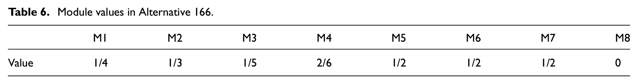
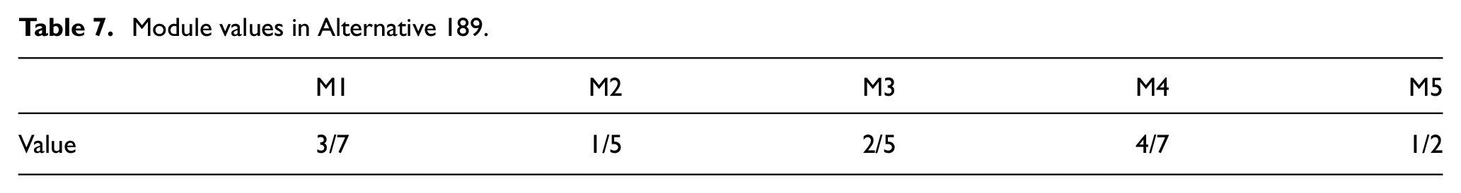
Table 4 shows the target values of the Pareto optimal solution sets of three goals. According to the concept of multiple objectives, these are the best solutions, but the target values of these solutions are different, and the decision will be made according to the engineer’s preference. As shown in Table 5, Alternative 166 is the solution to the 1-1-1 preference strategy, where the three objectives are of the same weight. The grouping result is shown in Figure 3. In contrast, Alternative 189 only considers the connection intensity, for which the grouping result of parts is shown in Figure 9. Compared with Alternative 189, Alternative 166 is better in both 3R1T and recycle benefit objectives, but its connection intensity score is not as good as that of Alternative 189. But Alternative 166 still takes the connection intensity of parts into consideration and maintains the balance of the three objectives. Therefore, if we consider three goals at the same time, the effects of objectives on the grouping result are evident. A balance is reached under the selection of preferences. From Tables 6 and 7, it can be seen that the values in Table 6 are better than those in Table 7, indicating that the recycle strategy in the module of Alternative 166 tends to be the same; some values are 0, meaning that the parts in this module have the same recycle strategy.

Figure 9.

The grouping result of Alternative 189.

Table 6.

Module values in Alternative 166.

	M1	M2	M3	M4	M5	M6	M7	M8
Value	1/4	1/3	1/5	2/6	1/2	1/2	1/2	0

Table 7.

Module values in Alternative 189.

	M1	M2	M3	M4	M5
Value	3/7	1/5	2/5	4/7	1/2

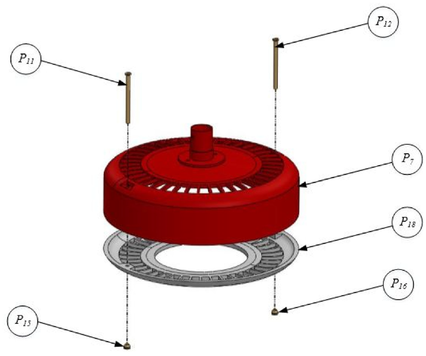
After reviewing the results for improvement, it is found that in Figure 3, Part 7 in Module 2 is different from Parts 4 and 6 in terms of recycle strategy, so it is decided to move Part 7 from Module 2 to Module 3. As shown in Figure 10, there are only Parts 4 and 6 in Module 2. Now the value of Module 2 changes from the original 1/3 to 0; that is, the recycle strategy of the parts in Module 2 is the same. The parts of Module 3 with Part 7 added are shown in Figure 11. It can be seen that Module 3 needs Parts 11, 12, 15, and 16 to connect Parts 7 and 18. If we improve the connection types of Parts 7 and 18, as shown in the parts of Module 3 in Figure 10, Module 3 cannot only eliminate the use of Parts 15 and 16 but also increase the recycle benefit from the original 12.1933 to 12.6671. By this redesign, we can reduce waste and increase the value of the recycle benefit.

Figure 10.

The redesigned ceiling fan parts.

Figure 11.

Add Part 7 to Module 3.

Conclusions

In the trend of customization and Design for a Green Life Cycle, modular research will help to trace the concept of the life cycle back to the source, product design, and resources can be employed more efficiently. This study attempts to provide a more complete systematic evaluation method for design strategies to make green product design more meaningful in its implementation. In this study, we explore the connection relationships, the cost-effectiveness, and three objectives of the 3R1T function in modules. Multi-objective genetic algorithms (MOGGAs) are used to derive the Pareto optimal solution in a quantitative way. Moreover, the designer’s preferences for different objectives are presented by a graphic interface, in which the designer can choose their preferences toward every objective so as to select alternatives that balance the multiple objectives from the optimal solution set. From the chosen solutions, the designer can improve the product design by adjusting the connection methods among parts to reduce differences in the recycle strategies within the module or to replace the materials of parts to change the recycle strategies. The results of the test example prove that the MOGGAs proposed in this study can effectively find the region of the Pareto optimal solution set to achieve the expected performance of modular design. From the modularization problem discussed in this study, in addition to the ceiling fan example, we also used the more complex stapler example (18 parts) to validate the feasibility of this method.

The assumptions in this study, such as the values of the connection intensity, are fixed and known, and they might be improved in the future. In addition, researchers can try to combine a CAD database with this method to make the modular planning more complete. Furthermore, the parameter settings will affect the solution searching time and the quality of the solution. In order to engage the full effectiveness of the algorithm, dynamic control of the parameters along with the stage of the algorithm should also be explored.

Footnotes

Appendix

Appendix C.

The disassembly costs of the ceiling fan parts.

	1	2	3	4	5	6	7	8	9	10	11	12	13	14	15	16	17	18	19	20	21	22	23	24	25	26
1	0.00	0.13	0.13	0.00	0.40	0.41	0.40	0.41	0.41	0.41	0.41	0.41	0.41	0.41	0.41	0.41	0.41	0.40	0.40	0.40	0.40	0.40	0.40	0.40	0.41	0.40
2	0.13	0.00	0.13	0.13	0.10	0.40	0.40	0.40	0.40	0.41	0.40	0.40	0.41	0.41	0.41	0.41	0.41	0.41	0.40	0.40	0.40	0.40	0.40	0.40	0.41	0.40
3	0.13	0.13	0.00	0.13	0.40	0.40	0.40	0.41	0.41	0.41	0.40	0.40	0.41	0.41	0.40	0.40	0.41	0.40	0.40	0.40	0.40	0.40	0.40	0.40	0.41	0.40
4	0.40	0.13	0.13	0.00	0.11	0.10	0.13	0.41	0.41	0.41	0.41	0.41	0.17	0.41	0.41	0.41	0.41	0.41	0.41	0.41	0.41	0.40	0.40	0.40	0.41	0.40
5	0.40	0.10	0.40	0.11	0.00	0.40	0.40	0.41	0.41	0.41	0.41	0.41	0.41	0.41	0.41	0.41	0.41	0.40	0.40	0.40	0.40	0.40	0.40	0.40	0.41	0.40
6	0.41	0.40	0.40	0.10	0.40	0.00	0.10	0.41	0.41	0.41	0.41	0.41	0.11	0.41	0.41	0.41	0.41	0.41	0.40	0.40	0.40	0.40	0.40	0.40	0.40	0.40
7	0.40	0.40	0.40	0.13	0.40	0.10	0.00	0.13	0.13	0.13	0.13	0.13	0.13	0.41	0.41	0.41	0.41	0.13	0.40	0.40	0.40	0.40	0.40	0.40	0.40	0.40
8	0.41	0.40	0.41	0.41	0.41	0.41	0.13	0.00	0.40	0.41	0.10	0.40	0.41	0.41	0.40	0.41	0.41	0.40	0.41	0.41	0.41	0.41	0.41	0.41	0.41	0.41
9	0.41	0.40	0.41	0.41	0.41	0.41	0.13	0.40	0.00	0.41	0.40	0.10	0.41	0.41	0.41	0.40	0.41	0.40	0.41	0.41	0.41	0.41	0.41	0.41	0.41	0.41
10	0.41	0.41	0.41	0.41	0.41	0.41	0.13	0.41	0.41	0.00	0.41	0.41	0.14	0.13	0.41	0.41	0.13	0.41	0.41	0.41	0.41	0.41	0.41	0.41	0.41	0.41
11	0.41	0.40	0.40	0.41	0.41	0.41	0.13	0.10	0.40	0.41	0.00	0.40	0.41	0.41	0.10	0.40	0.41	0.13	0.40	0.40	0.40	0.40	0.40	0.40	0.40	0.40
12	0.41	0.40	0.40	0.41	0.41	0.41	0.13	0.40	0.10	0.41	0.40	0.00	0.41	0.41	0.40	0.10	0.41	0.13	0.40	0.40	0.40	0.40	0.40	0.40	0.40	0.40
13	0.41	0.41	0.41	0.17	0.41	0.11	0.13	0.41	0.41	0.14	0.41	0.41	0.00	0.40	0.41	0.41	0.14	0.41	0.40	0.40	0.40	0.40	0.40	0.40	0.16	0.40
14	0.41	0.41	0.41	0.41	0.41	0.41	0.41	0.41	0.41	0.13	0.41	0.41	0.40	0.00	0.41	0.41	0.13	0.41	0.40	0.40	0.40	0.40	0.40	0.40	0.40	0.40
15	0.41	0.41	0.40	0.41	0.41	0.41	0.41	0.40	0.41	0.41	0.10	0.40	0.41	0.41	0.00	0.40	0.41	0.13	0.40	0.40	0.40	0.40	0.40	0.40	0.40	0.40
16	0.41	0.41	0.40	0.41	0.41	0.41	0.41	0.41	0.40	0.41	0.40	0.10	0.41	0.41	0.40	0.00	0.41	0.13	0.40	0.40	0.40	0.40	0.40	0.40	0.40	0.40
17	0.41	0.41	0.41	0.41	0.41	0.41	0.41	0.41	0.41	0.13	0.41	0.41	0.14	0.13	0.41	0.41	0.00	0.41	0.13	0.13	0.13	0.13	0.13	0.13	0.40	0.40
18	0.40	0.41	0.40	0.41	0.40	0.41	0.13	0.40	0.40	0.41	0.13	0.13	0.41	0.41	0.13	0.13	0.41	0.00	0.40	0.40	0.40	0.40	0.40	0.40	0.40	0.40
19	0.40	0.40	0.40	0.41	0.40	0.40	0.40	0.41	0.41	0.41	0.40	0.40	0.40	0.40	0.40	0.40	0.13	0.40	0.00	0.40	0.40	0.10	0.40	0.40	0.41	0.40
20	0.40	0.40	0.40	0.41	0.40	0.40	0.40	0.41	0.41	0.41	0.40	0.40	0.40	0.40	0.40	0.40	0.13	0.40	0.40	0.00	0.40	0.40	0.10	0.40	0.41	0.40
21	0.40	0.40	0.40	0.41	0.40	0.40	0.40	0.41	0.41	0.41	0.40	0.40	0.40	0.40	0.40	0.40	0.13	0.40	0.40	0.40	0.00	0.40	0.40	0.10	0.41	0.40
22	0.40	0.40	0.40	0.40	0.40	0.40	0.40	0.41	0.41	0.41	0.40	0.40	0.40	0.40	0.40	0.40	0.13	0.40	0.10	0.40	0.40	0.00	0.40	0.40	0.41	0.40
23	0.40	0.40	0.40	0.40	0.40	0.40	0.40	0.41	0.41	0.41	0.40	0.40	0.40	0.40	0.40	0.40	0.13	0.40	0.40	0.10	0.40	0.40	0.00	0.40	0.41	0.40
24	0.40	0.40	0.40	0.40	0.40	0.40	0.40	0.41	0.41	0.41	0.40	0.40	0.40	0.40	0.40	0.40	0.13	0.40	0.40	0.40	0.10	0.40	0.40	0.00	0.41	0.40
25	0.41	0.41	0.41	0.41	0.41	0.40	0.40	0.41	0.41	0.41	0.40	0.40	0.16	0.40	0.40	0.40	0.40	0.40	0.41	0.41	0.41	0.41	0.41	0.41	0.00	0.12
26	0.40	0.40	0.40	0.40	0.40	0.40	0.40	0.41	0.41	0.41	0.40	0.40	0.40	0.40	0.40	0.40	0.40	0.40	0.40	0.40	0.40	0.40	0.40	0.40	0.12	0.00

Declaration of conflicting interests

The author(s) declared no potential conflicts of interest with respect to the research, authorship, and/or publication of this article.

Funding

The author(s) disclosed receipt of the following financial support for the research, authorship, and/or publication of this article: This research was supported by the Ministry of Science and Technology of the Republic of China under grant number MOST 108-2410-H-167-003.

ORCID iD

Hwai-En Tseng

References

Otto

Wood

. Product design-technical in reverse engineering and new product development. London: Prentice Hall, 2001.

Jose

Tollenaere

. Modular and platform methods for product family design: literature analysis. J Intell Manuf 2005; 16: 371–390.

Bonvoisin

Halstenberg

Buchert

, et al. A systematic literature review on modular product design. J Eng Des 2016; 27(7): 488–514.

Piran

FAS

Lacerda

Antunes

JAV

, et al. Modularization strategy: analysis of published articles on production and operations management (1999 to 2013). Int J Adv Manuf Technol 2016; 86(1–4): 507–519.

Sonego

Echeveste

MES

Galvan Debarba

. The role of modularity in sustainable design: a systematic review. J Clean Prod 2018; 176: 196–209.

Huang

Kusiak

. Modularity in design of products and systems. IEEE Trans Syst Man Cybern A Syst Hum 1998; 28(1): 66–77.

Kreng

Lee

. Modular product design with grouping genetic algorithm—a case study. Comput Ind Eng 2004; 46: 443–460.

Lei

Peng

Lei

, et al. A similarity analysis method of the non-isomorphism generalized module in product platform. Proc IMechE, Part B: J Engineering Manufacture 2018; 232(2): 358–370.

Bhosekar

Ierapetritou

. Modular design optimization using machine learning-based flexibility analysis. J Process Control 2020; 90: 18–34.

10.

Gunji

Deepak

BBBVL

Bahubalendruni

CMVAR

, et al. An optimal robotic assembly sequence planning by assembly subsets detection method using teaching learning-based optimization algorithm. IEEE Trans Autom Sci Eng 2018; 15(3): 1369–1385.

11.

Gulivindala

Bahubalendruni

MVR

Varupala

SSVP

, et al. A heuristic method with a novel stability concept to perform parallel assembly sequence planning by subassembly detection. Assem Autom 2020; 40(5): 779–787.

12.

Park

Yoon

, et al. Integration of axiomatic design and design structure matrix for the modular design of automobile parts. Proc IMechE, Part B: J Engineering Manufacture 2022; 236(3): 296–306.

13.

Wei

. Modular design for optimum granularity with auto-generated DSM and improved elbow assessment method. Proc IMechE, Part B: J Engineering Manufacture 2022; 236(4): 413–426.

14.

Zhang

Gershenson

. An initial study of direct relationships between life-cycle modularity and life-cycle cost. Concurr Eng 2003; 11(2): 121–128.

15.

Fujita

Yoshida

. Product variety optimization simultaneously designing module combination and module attributes. Concurr Eng 2004; 12(2): 105–118.

16.

Tseng

Chang

Cheng

. Disassembly-oriented assessment methodology for product modularity. Int J Prod Res 2010; 48(14): 4297–4320.

17.

Agrawal

Sao

Fernandes

, et al. A hybrid model of component sharing and platform modularity for optimal product family design. Int J Prod Res 2013; 51(2): 614–625.

18.

Newcomb

Bras

Rosen

. Implications of modularity on product design for the life cycle. J Mech Des 1998; 120: 483–490.

19.

Sosale

. Product modularization for life cycle engineering. Robot Comput Integr Manuf 1999; 15: 387–401.

20.

Tseng

Chang

. Modular design to support green life-cycle engineering. Expert Syst Appl 2008; 34(4): 2524–2537.

21.

Smith

Yen

. Green product design through product modularization using atomic theory. Robot Comput Integr Manuf 2010; 26(6): 790–798.

22.

Yang

Tao

, et al. Product modular design incorporating life cycle issues - group genetic algorithm (GGA) based method. J Clean Prod 2011; 19: 1016–1032.

23.

Yan

Feng

. Sustainable design-oriented product modularity combined with 6R concept: a case study of rotor laboratory bench. Clean Technol Environ Policy 2014; 16(1): 95–109.

24.

Ameli

Mansour

Ahmadi-Javid

. A sustainable method for optimizing product design with trade-off between life cycle cost and environmental impact. Environ Dev Sustain 2017; 19(6): 2443–2456.

25.

Yang

Sekhari

. A modular eco-design method for life cycle engineering based on redesign risk control. Int J Adv Manuf Technol 2011; 56: 1215–1233.

26.

You

Smith

. A multi-objective modular design method for creating highly distinct independent modules. Res Eng Des 2016; 27: 179–191.

27.

Abido

Elazouni

. Modified multi-objective evolutionary programming algorithm for solving project scheduling problems. Expert Syst Appl 2021; 183: 115338.

28.

Ishibuchi

Yoshida

Murata

. Balance between genetic search and local search in memetic algorithms for multi-objective permutation flowshop scheduling. IEEE Trans Evol Comput 2003; 7: 204–223.

29.

Bahubalendruni

Biswal

. A review on assembly sequence generation and its automation. Proc IMechE, Part C: J Mechanical Engineering Science 2016; 230(5): 824–838.

30.

Bahubalendruni

MVAR

Biswal

. An efficient stable subassembly identification method towards assembly sequence generation. Natl Acad Sci Lett 2018; 41(6): 375–378.

A multi-objective grouping genetic algorithm for modular design

Abstract

Keywords

Introduction

Methodology

Assumption and procedure in MOGGAs

Multi-objectives for modular design

3R1T

Connection intensity

Recycle benefits

Multi-objective grouping genetic algorithms (GGAs)

Encoding and initial solution to GGAs

Crossover and mutation mechanisms

The Pareto optimal solution set

The user interface

Simulation testing

Test results and analysis

Discussion and modification

Conclusions

Footnotes

Appendix

Declaration of conflicting interests

Funding

ORCID iD

References