Sage Journals: Discover world-class research

Abstract

In this paper, a universal method is proposed to accurately identify wheel state during grinding brittle materials. In contrast with conventional methods relying on adequate repetitive experimental data under the same process conditions, only history acoustic emission (AE) data in the same life cycle of a grinding wheel are needed for current wheel state identification. During grinding process, AE spectra samples are acquired sequentially on a series of nodes with equal interval. Samples on each node are categorized into the same class of wheel state. In the theoretical part, AE spectrum is proved to be suitable for feature representation of the degradation of wheel condition. Linear discriminant analysis is used to project AE spectra samples into a two-dimensional feature space, and the changes of the projection gives a clue to the evolution of wheel state. Two types of commonly used diamond wheels for optical surface grinding, which are straight wheel and cup wheel, were used to verify the general applicability of the method. The experiments were carried out on different machine tools and the two wheels also possessed different degradation process, yet for all of them, the evolution of wheel state can be accurately identified. It was proved that the proposed method can adaptively trace wear stage change of diamond grinding wheel.

Keywords

Grinding wheel wear acoustic emission signal brittle material

Introduction

The grinding process is one of the common methods to achieve high quality of large-scale optical surface. A worn wheel can lead to unscheduled downtime and damage to workpiece, and timely dressing is essential for efficiency and cost.¹ However, wheel condition monitoring is a thorny problem in practice. Abrasive grains on wheel surface are random in size, shape and orientation, which makes grinding process more complex compared with cutting and drilling with deterministic tools. Indirect grinding monitoring methods relying on diverse sensors have been widely employed in the controlling and optimizing of grinding process.^2–4 Among all of the process variables, acoustic emission (AE) signal is prominent for its fast response and high sensitivity.⁵ AE is an elastic stress wave generated within a material when it undergoes deformation and fracture.⁶ Abrasive grains protruding from wheel surface will rub, plow, or cut the material during grinding. All of these micro interaction behaviors may cause changes on wheel and material, and correspondingly induce AE events with different mechanisms. Therefore, AE is more subtle and sensitive than other process variables such as force, vibration, temperature, and etc.

Because of its excellent characteristics, AE-based monitoring attracted a lot of research attention. Statistical features such as root-mean-square and ring-down count are always used as monitoring parameters,^7–9 and features in frequency domain or time-frequency domain are alternative choices for grinding and dressing process monitoring.^10–12 Although these artificial simple features have been proved effective in some specific instances, the major drawback of them is their strong dependence on the threshold. Considering the disadvantages of conventional features, researchers also proposed some innovative features of AE signals based on modern signal processing techniques.^13,14

In fact, there may be a lot of try and error before achieving appropriate features for monitoring when relying on signal processing techniques for feature extraction. Grinding process is a time-varying process with topography of wheel continuously changing, which determines the randomness of AE signals. The nonuniformity of material and the original flaws on or beneath the surface make grinding mechanisms more complex, especially for brittle materials.¹⁵ Therefore, it is hard to figure out whether the extracted features are the optimal choice for monitoring. Feature selection is further studies for more elaborate monitoring of grinding wheel condition. Liao¹⁶ collected AE signals during grinding ceramic materials and processed them by autoregressive modeling or discrete wavelet decomposition for feature extraction. The best feature subsets were found by three different feature selection methods, including two proposed ant colony optimization based method and the sequential forward floating selection method.

The ambiguous relationship between characteristic features and wheel wear makes data-driven models very popular for wheel condition monitoring. Lezanski¹⁷ extracted statistical and spectral features from forces, vibration, and AE. A feed-forward back propagation neural network was built for feature selection, and a neuro-fuzzy model was trained for grinding wheel condition classification. Nakai et al.¹⁸ compared four types of artificial neural networks (MLP, RBF, GRNN, and ANFIS) on wheel wear estimation. AE signals, power signals, and statistics derived from them were taken as the input features of the models. Surface roughness of workpiece was the output in the consideration of its close relationship with wheel wear. Krishnan and Rameshkumar¹⁹ employed AE-RMS features to build Hidden Markov Models of wheel condition. Three tool states such as “sharp,”“intermediate,” and “worn out” were predicted with good accuracy. Liao et al.²⁰ utilized AE features to identify dull wheel. The minimum distance classifier was the weak learner and two types of booting algorithms (AdaBoost and A-Boost) were employed to enhance the effect of the classification. Lee et al.²¹ utilized a microphone embedded in the grinding machine to collect audio signals during the grinding process. The most discriminated feature was extracted from spectrum analysis and a deep convolutional neural network was trained to distinguish sharp and worn wheel. Guo et al.²² selected optimal feature subset from a large quantity of features of AE, grinding force, and vibration and used Long Short-Term Memory network to predict wheel wear.

The literature review showed that grinding wheel wear estimation was always modeled as a classification problem. Binary or ternary classification was the common choice. Wheel state was always classified as early wear stage, normal wear stage, or serious wear stage. There were still some research that suggested one or two intermediate state during normal wear stage for more accuracy. However, rough classification is not enough for the situation of high requirement on the stability of wheel condition. Grinding with diamond wheel is a common process for large scale optical components. In order to avoid unpredictable catastrophic damages on and beneath the ground surface, consistent grinding wheel condition is necessary.^23–25 Fine classification or regression well-trained models are competent for the purpose. But the modeling is hard to be realized, not only for the difficulty of acquiring sufficient training data, but also for the difficulty of precisely labeling. Numerical labels of training data must be able to reflect wheel state evolution objectively. But even so, the well-trained model is still hardly adaptive to a new life cycle of the wheel due to the diverse uncertainties in the dressing process of grinding wheel.²⁶ Initial topography of wheel and the degradation of grinding performance are different for different life cycles, even if the same dressing parameters are adopted.

Considering the above factors, modeling wheel state evaluation as a regression or a fine classification problem is a tough work and the monitoring accuracy is probably unsatisfactory in practical grinding brittle material. In this paper, a universal method of tracking the evolution process of wheel state is proposed based on acoustic emission (AE) signals. Precision grinding of brittle materials with diamond wheel is the study focus. In the second section, the component of AE signals in brittle material grinding is analyzed from the view of generation mechanism. AE spectrum is proved to be appropriate for feature representation. And linear discriminant analysis (LDA) is used to project spectra of AE samples into a two-dimensional feature space for visualization. Monitoring strategy which only relying on history and current AE samples in the same life cycle of a wheel is introduced in this section based on above theory analysis. In order to verify the effectiveness of the proposed method, whole life cycle experiments of a straight wheel and a cup wheel were carried out on two grinding machines. These two kinds of wheels are commonly used diamond wheels for optical surface grinding. Experimental results show that detailed stages of the evolution of wheel condition can be distinguished, no matter what kind of wear types they were.

Basic theory

Characteristics of AE signals in frequency domain

There are two types of AE signals during grinding brittle material: burst-type AE (b-AE) and continuous-type AE (c-AE).²⁷ B-AE induced by crack propagation and material breakage is predominant during removing brittle material under brittle regime. C-AE associated with friction and deformation always has a quite low energy in contrast with b-AE. Therefore, only b-AE signals are concerned for AE feature representation in the next section.

Waveform of a b-AE event is characterized by high frequency oscillation and fast attenuation. A b-AE from a certain AE source can be simply simulated as $A e^{- α t} \cos ω t$ where A and $α$ represent the amplitude and the attenuating factor of the AE event, respectively. The sign $ω$ is the oscillation frequency. During grinding process, a variable number of abrasive grains with irregular cutting edges are involved in grinding interaction. Some b-AE events may be induced simultaneously, and the sum is $\sum_{i = 1}^{I} A_{i} e^{- α_{i} t} \cos ω_{i} (t)$ . New AE events probably burst out before previous ones are completely exhausted. Therefore, AE signal picked up by an AE sensor in time span $[0, T]$ is the overlap of all b-AE events within the period. Suppose $t_{q} (q = 1, 2, \dots Q)$ are occurrence time points of b-AE events during the time span, with the aid of the unit step function $u (t)$ , AE signal $x (t)$ can be represented as follows:

\begin{matrix} x (t) = \sum_{q = 1}^{Q} \sum_{i = 1}^{I} [A_{qi} e^{- α_{qi} (t - t_{q})} \cos ω_{qi} (t - t_{q})] u (t - t_{q}) \\ where u (t) = {\begin{matrix} 1 & t \geq 0 \\ 0 & t < 0 \end{matrix} and α_{qi} > 0, A_{qi} \geq 0 \end{matrix}

(1)

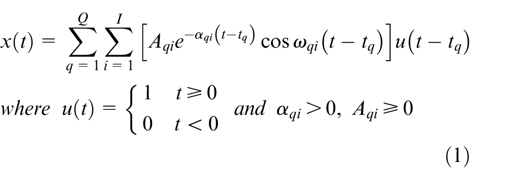
The sign I represents the number of b-AE events occurred on a certain time point $t_{q}$ . In fact, the actual number of abrasive grains which are involved in the grinding interaction on a certain time point is uncertain. For a uniform equation, $A_{qi}$ is allowed to be zero for some circumstance. According to the convolution theorem in frequency domain, the Fourier transform of $x (t)$ is:

\begin{matrix} X (ω) = \sum_{q = 1}^{Q} \sum_{i = 1}^{I} \frac{e^{- j ω t_{q}}}{2 π} \\ {\frac{A_{qi}}{α_{qi} + j ω} \otimes [π δ (ω - ω_{qi}) + π δ (ω + ω_{qi})]} \end{matrix}

(2)

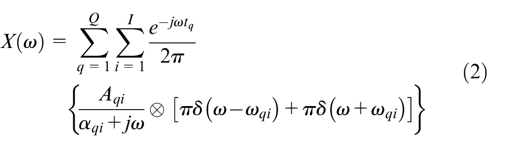
where the sign ⊗ represents the convolution operation and $δ$ is the Dirac delta function. According to the basic properties of $δ$ , $X (ω)$ in the positive frequency domain can be rewritten as:

X_{half} (ω) = \sum_{q = 1}^{Q} \sum_{i = 1}^{I} \frac{\frac{1}{2} A_{qi} e^{- j ω t_{q}}}{α_{qi} + j (ω - ω_{qi})} = \sum_{q = 1}^{Q} \sum_{i = 1}^{I} P_{qi} (ω) e^{- j ω t_{q}}

(3)

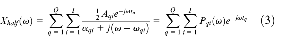
For each component $P_{qi} (ω)$ in equation (3), the amplitude is shown as:

| P_{qi} (ω) | = \frac{\frac{1}{2} A_{qi}}{\sqrt{α_{qi}^{2} + {(ω - ω_{qi})}^{2}}}

(4)

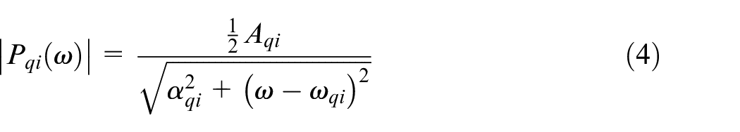
It shows that the amplitude of each component in $x (t)$ decreases rapidly with the frequency factor $ω$ far away from the symmetry center $ω_{qi}$ . In other words, energy of each component concentrates in a limited frequency band centered by the corresponding oscillation frequency $ω_{qi}$ . In grinding process, the primary b-AE sources are the initiation and propagation of cracks in material, removal of material, breakage, and pulling out of abrasive grains. Different types of b-AE components have various oscillation frequency. Therefore, their energies concentrate in different frequency spans because of their localization in frequency domain.

If considering all possible values of oscillation frequency, the frequency spectrum of AE signal is supposed to be wide band. But in fact, spectrum energy is always distributed in several frequency span as shown in the experiment section. According to the linear superposition of b-AE components shown in equation (3), there must be several main types of b-AE components with approximate equal oscillation frequencies. B-AE components with different mechanisms mixed in time domain are separated to some extent in frequency domain.

Oscillation frequency of b-AE is determined by the size of crack and chip which is related to the state of abrasive grains on wheel surface.²⁸ It is hard to figure out the relationship between fracture mechanisms and AE mechanisms because patterns of b-AE are influenced by specific damage accumulation of the ground material.^29,30 However, an undeniable fact is that the changing state of grains during grinding process results in the changes of the major fracture mechanisms, and correspondingly the changes of major types ofb-AE components and the proportion among them. Therefore, considering the separation of different types of b-AE components in frequency domain, AE spectrum is suitable for the identification of wheel state evolution. In the following section, AE spectrum will be taken as the original feature vector and LDA will be used to distinguish AE samples from various classes to the maximum extent possible.

Dimensionality reduction of AE spectrum based on LDA

The dimensionality of frequency spectrum of AE signals is super high because of the characteristic of stochastic and broadband. In order to evaluate wheel state fast and conveniently, low dimensional features are needed for monitoring. PCA (Principal Component Analysis) and LDA are commonly used methods for dimensionality reduction in machine learning.^31–34 Both of them are linear transformation techniques and the difference is that LDA is a supervised whereas PCA is unsupervised. PCA is a technique that finds the directions of maximal variance. In contrast, LDA attempts to find a feature subspace that maximizes class separability.³⁵ Because of the characteristic of LDA, in this paper, LDA is employed for dimensionality reduction of AE spectrum. And reduction features will be directly used for wheel condition monitoring.

The basic idea of LDA is to project all samples on a low-dimensional feature space on the premise that samples in the same class are as close as possible and at the same time different classes are far away from each other as much as possible. For a given dataset $D = {(x_{i}, y_{i})}, y_{i} \in {1, \dots, N}$ , $x_{i} \in R^{d}, i = 1, 2, \dots, m$ , there are N types of samples corresponding to set $X_{j}$ where $j = 1, 2, \dots, N$ . Suppose $μ$ is the mean vector of all samples in D, and $μ_{j}$ is the mean vector of samples in set $X_{j}$ , the global scatter matrix $S_{t}$ , the with-in class scatter matrix $S_{w}$ , and the between-class scatter matrix $S_{b}$ are defined respectively as follows³⁶:

S_{t} = \sum_{i = 1}^{m} (x_{i} - μ) {(x_{i} - μ)}^{T}

(5)

S_{w} = \sum_{j = 1}^{N} \sum_{x_{i} \in X_{j}} (x_{i} - μ_{j}) {(x_{i} - μ_{j})}^{T}

(6)

S_{b} = S_{t} - S_{w}

(7)

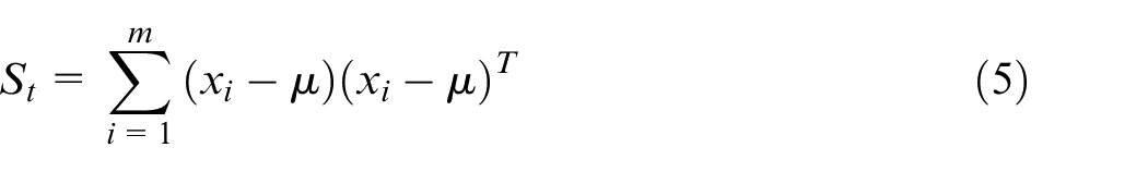
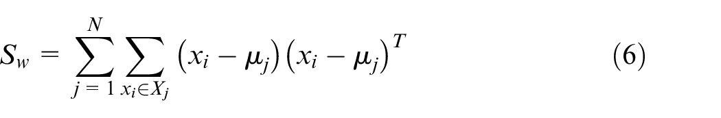
Substitute equations (5) and (6) into equation (7), and $S_{b}$ can be rewritten as:

S_{b} = \sum_{j = 1}^{N} m_{j} (μ_{j} - μ) {(μ_{j} - μ)}^{T}

(8)

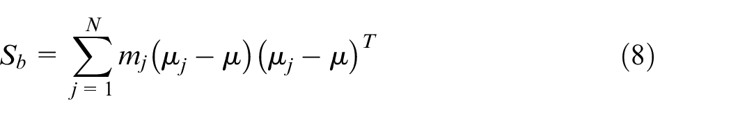
For a linearly separable dataset including N classes, $N - 1$ times of projections are sufficient for separating classes from each other. The optimization target of LDA can be represented as follows:

max_{γ_{q}} J = \frac{\sum_{q = 1}^{N - 1} {γ_{q}}^{T} S_{b} γ_{q}}{\sum_{q = 1}^{N - 1} {γ_{q}}^{T} S_{w} γ_{q}}

(9)

where $γ_{q} \in R^{d}$ is the projection direction vector. The numerator and the denominator in equation (9) are all quadratic form of $γ_{q}$ . Therefore, without loss of generality, the optimization problem can be rewritten as follows:

\begin{matrix} min_{γ} - \sum_{q = 1}^{N - 1} {γ_{q}}^{T} S_{b} γ_{q} \\ s . t . \sum_{q = 1}^{N - 1} {γ_{q}}^{T} S_{w} γ_{q} = 1 \end{matrix}

(10)

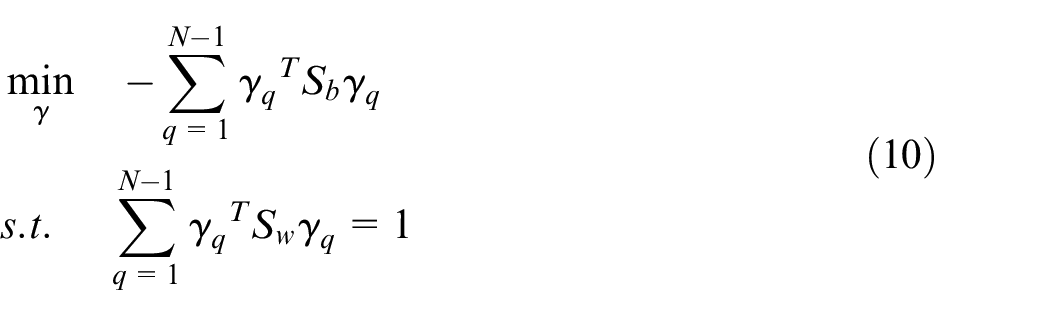
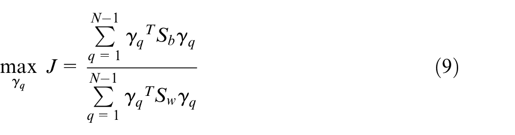
The optimal value of $γ_{q} (q = 1, 2, \dots, N - 1)$ is the first $N - 1$ eigen vectors of the matrix ${S_{w}}^{- 1} S_{b}$ and they are sorted according to the corresponding eigenvalues from big to small. In LDA, these eigen vectors are commonly known as linear discriminants. Using the coordinate transformation matrix composed by the linear discriminants, the original high-dimensional feature vector can be projected on a low-dimensional feature space.

Monitoring strategy for wheel state evolution

No matter what kind of wear type of grinding wheel, wheel wear process is conventionally divided into three stages, early wear stage, normal wear stage, and serious wear stage. Early wear stage means initial quick wear because of the instability of wheel topography just after dressing. After that, wheel enters a stable development stage which is named as the normal wear stage. When the wheel approaches its life end, severe interaction between wheel and material induces accelerated wear, and it is the serious wear stage. It is clear that the division of wheel wear stages is based primarily on the change degree of wheel state. For more precision, wheel state is not continuously deteriorate during grinding. Serious abrasion of abrasive grains may cause cracks on grains and bond. The appearance of new cutting edges and new grains will make a recovery of the grinding performance to some extent. Although it is hard to measure the extent of the recovery, whether the current state is better or worse can be judged by comparing the situation before and after it. Therefore, the time sequence of samples of process variables is worthy for performance degradation evaluation, and it is always neglected for classification and regression models trained by labeled samples. Continuously acquiring AE samples with the elapse of grinding time, AE features will change with the evolution of wheel state. Measuring the difference of adjacent samples will give a clue for the tracking of wheel state evolution.

Grinding process is a stochastic process. Decision-making based on a single AE sample and its neighbors is unreliable. Considering the super high acquisition frequency, plenty of AE samples can be acquired within a short time span in which the change of wheel state is insignificant. A series of nodes with the same interval can be preset on the timeline, and AE samples are only acquired on these nodes. Time consumption of collecting AE samples on each node is quite short compared with the interval. Therefore, AE samples acquired on each node share the same label and correspond to the same wheel state. Classification and regression models always adopt physical-meaningful labels, however, labeling deduced from specific signal features is hardly objective and widely adaptive especially for fine classification and regression. As above mentioned, the time sequence of AE samples is important for degradation evaluation. Therefore, concern for relative changes of AE samples along the timeline, instead of the specific signal features, is the basic principle of the proposed monitoring strategies.

Considering the evolution of wheel state under variable process parameters, material removal volume (MRV) interval instead of time interval is finally adopted for AE samples acquisition in this paper. MRV is more objective to represent the consuming of wheel during grinding process. AE samples picked up on a certain node are put into a data subset and the sequence number is simply taken as its label. With the elapse of grinding time, more and more subsets are acquired. On each node, LDA is used to project all available subsets on a low-dimensional feature space. If wheel state gets some obvious changes at the current node, sample features of the current subset will be very different from those before. The principle of LDA is to separate samples of different classes to the maximum extent. Therefore, the optimal projection directions will alter for the biggest extent discrimination. The projection pattern will be quite different compared with the situation of the previous node, and the current subset will separate from previous subsets. According to feature projection and its evolution, the transformation of wheel state can be timely identified.

Experiments

Experimental instruments and parameters

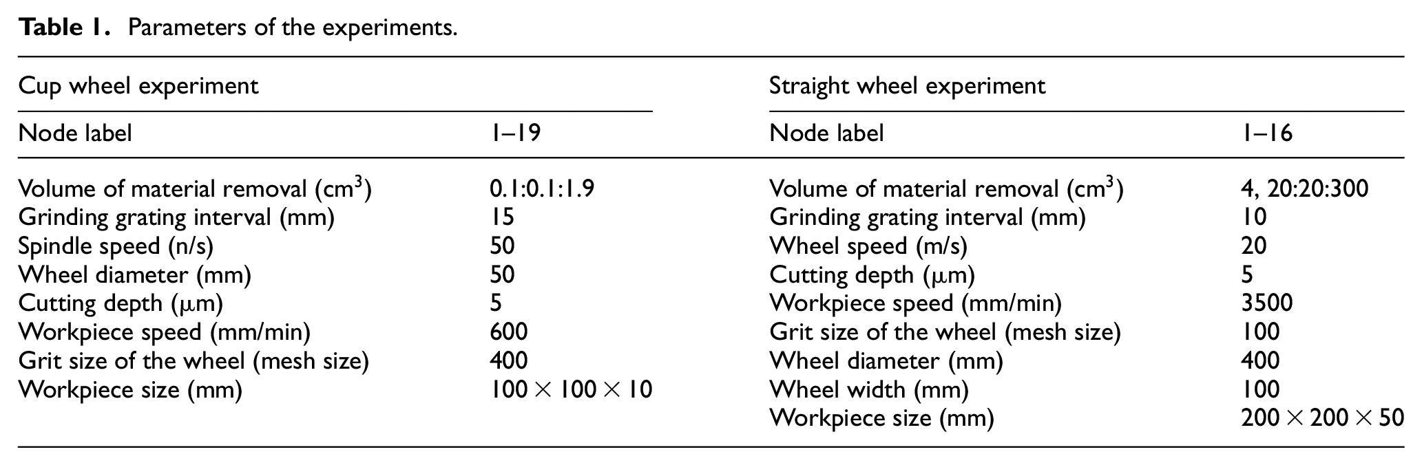
Surface grinding experiments of a cup wheel and a straight wheel were carried out on different grinding machines. The two wheels were all resin bond diamond wheel. Fused silica glass was ground under water soluble cooling fluid. Experimental instruments of the two experiments are shown in Figures 1 and 2, respectively. Specimens were adhered to the workbench and grating scanning path was adopted during grinding. Other experimental parameters are listed in Table 1. R50A AE sensors were fixed on the workbench and PCI-2 acoustic emission acquisition system of Physical Acoustics Corporation were used to acquire AE samples and the acquisition frequency was 1 MHz for the two experiments. 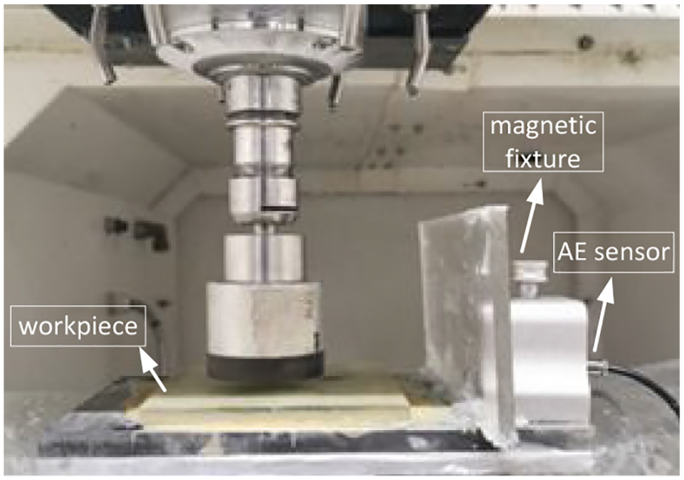AE signal was continuously picked up on each node, and then it was divided into $10 ms$ length data segments. Data samples acquired on a certain node were classified into the same class of wheel state. The sampling time length on each node was several seconds, while the time interval of adjacent nodes was several minutes. Therefore, it was reasonable to suppose unchanged wheel state for AE samples on each node.

Figure 1.

Experimental instruments of the first experiment.

Figure 2.

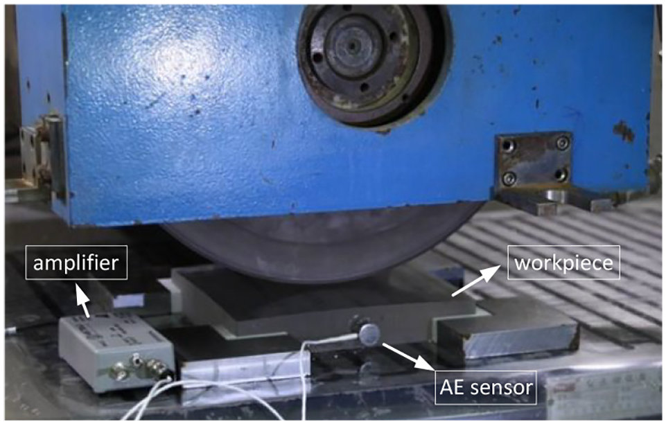
Experimental instruments of the second experiment.

Table 1.

Parameters of the experiments.

Cup wheel experiment		Straight wheel experiment
Node label	1–19	Node label	1–16
Volume of material removal ( $c m^{3}$ )	0.1:0.1:1.9	Volume of material removal ( $c m^{3}$ )	4, 20:20:300
Grinding grating interval (mm)	15	Grinding grating interval (mm)	10
Spindle speed (n/s)	50	Wheel speed (m/s)	20
Wheel diameter (mm)	50	Cutting depth (µm)	5
Cutting depth (µm)	5	Workpiece speed (mm/min)	3500
Workpiece speed (mm/min)	600	Grit size of the wheel (mesh size)	100
Grit size of the wheel (mesh size)	400	Wheel diameter (mm)	400
Workpiece size (mm)	100 × 100 × 10	Wheel width (mm)	100
		Workpiece size (mm)	200 × 200 × 50

For the purpose of verification, topography images on some fixed locations of the two wheels were picked up during grinding. And part of them are shown in Figures 3 and 4, respectively. Wheel topography got an obvious change for the first experiment and serious blocking of workpiece materials on the wheel surface can be recognized at the end of the experiment. The circumstance is quite different for the second experiment. It was carried out on a self-designed high precision grinding machine and all conditions were as the same as those of grinding large scale optical lens. In addition to slightly expanding wear plane area on abrasive grains, the wheel topography didn’t get obvious changes during the experiment. Abrasive grain abrasion was the dominant wear type. The majority of abrasive grains protruding from the wheel surface survived for the whole grinding process and wear plane on them slightly enlarged gradually. Several pull-out and new grains can be recognized by elaborate comparison between images on the same location. After the 16th node, a visible damage suddenly occurred on the ground surface. Wheel topography was almost the same before and after the workpiece was broken. Catastrophic damages always occur without any warning during grinding brittle materials. That is also why more sensitive monitoring is required during grinding optical components.

Figure 3.

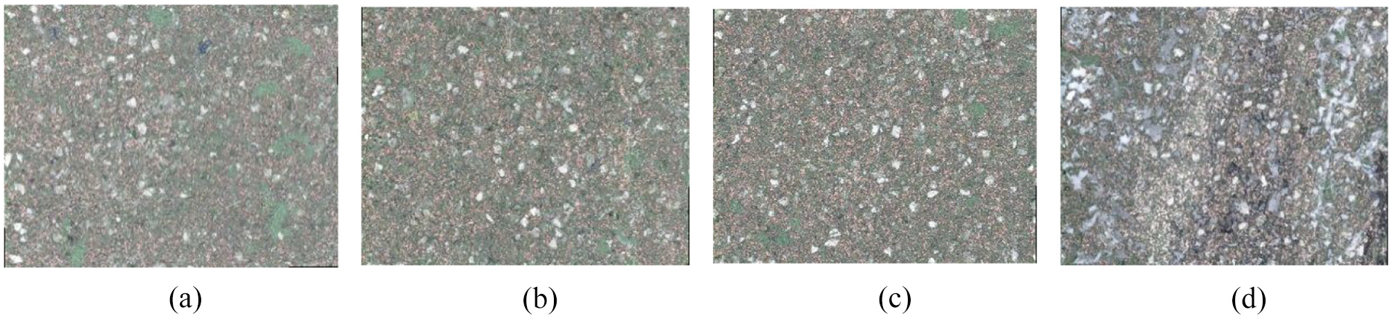
Topography images of the cup wheel (magnified 500 times): (a) the 5th node, (b) the 13th node, (c) the 17th node, and(d) the 19th node.

Figure 4.

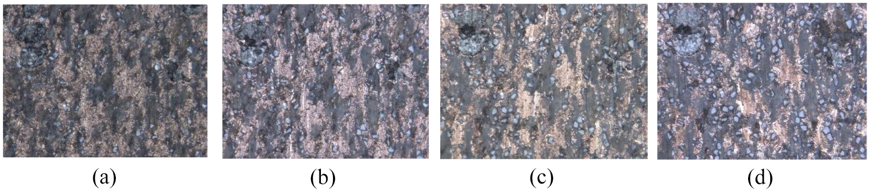
Topography images of the straight wheel (magnified 500 times): (a) the 2nd node, (b) the 5th node, (c) the 11th node, and (d) the 16th node.

Frequency spectra of some AE samples of the two experiments are shown in Figures 5 and 6, respectively. It was broadband and energy was concentrated on some frequency spans. It coincides with the above theoretical analysis, different types of AE components concentrate in different frequency spans. With the elapse of grinding time, spectrum pattern got some changes but there were not obvious features which can represent the deterioration of wheel wear. Spectrum pattern changes because of the varying proportion of diverse b-AE mechanisms in AE signals. The proportion is basically invariable in terms of statistics if wheel state remains the same. Therefore, AE spectra in the same subset acquired on a certain node were quite similar in amplitude and energy distribution. Although AE spectra were full of information of wheel wear, it was still hard to clarify wheel wear extent from their evolution. Next, LDA is used to distinguish between them.

Figure 5.

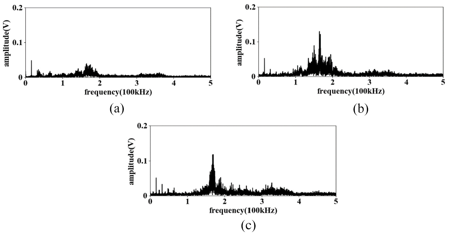
Spectra of AE samples on different nodes of the first experiment: (a) the 1st node, (b) the 7th node, and (c) the 19th node.

Figure 6.

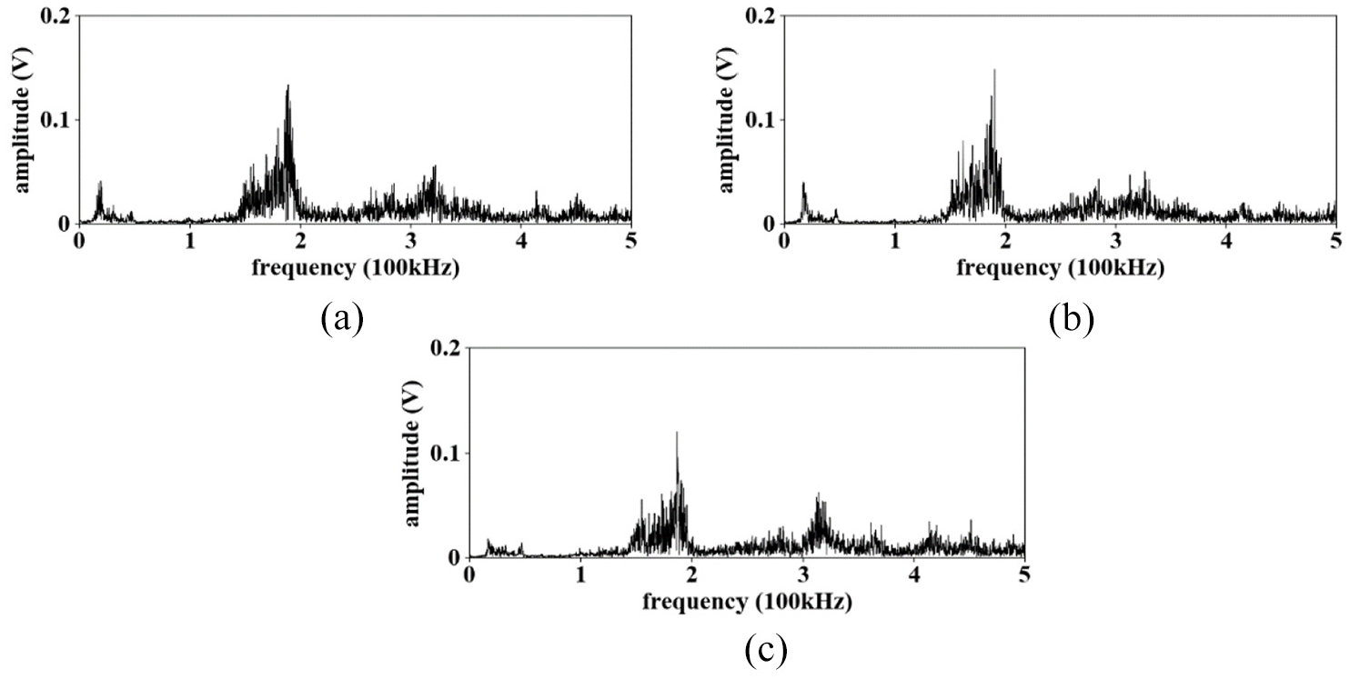
Spectra of AE samples on different nodes of the second experiment: (a) the 1st node, (b) the 9th node, and (c) the 16th node.

Wheel wear monitoring by reduced dimensional features of AE signals

For the purpose of online monitoring, once AE samples of the current node were acquired, spectra of history and current samples were projected on a two-dimensional feature space by LDA. LDA can be implemented conveniently by employing Scikit-learn toolbox in Python.³⁷ According to the principle of LDA, a linearly separable dataset including N classes can be totally separated through N−1 times projection. It is difficult for visualization when the dimensionality is above three. Besides, entirely discriminating wheel state on each node is not necessary for wheel condition monitoring. According to the law of wheel state evolution, wheel condition will deteriorate in general and intersperse several times minor recoveries caused by self-sharpening. The concerned problem in wheel condition monitoring is the difference of the current state from before as mentioned in section 2.3. Therefore, only the first two linear discriminants were retained for LDA and the following result analysis also shows that it is sufficient to identify wheel wear evolution.

The case of the first experiment is shown in Figure 7. If only the first two linear discriminants were retained for LDA, the spectrum series of an AE sample is concentrated on a point. The projection of a dataset is a cluster of scattered points in the two-dimensional space. Therefore, the LDA results are some scatterplots as shown in Figure 7(a) to (i). Similar characteristics of AE samples from the same nodes made their projection points get together and each data subset corresponding to each node is a clustering point cloud. Different subsets are represented with different color and mark. Numbers in the legends represent node labels which are listed in Table 1. On each node, a data subset represented the current state of the wheel was picked up. Then all available subsets, including reserved history ones and the current one, were re-projected on the two dimensional feature space by LDA. The results on a series of nodes are shown in Figure 7(a) to (i), respectively. The first two linear discriminants are simplified to LD1 and LD2 in these plots.

Figure 7.

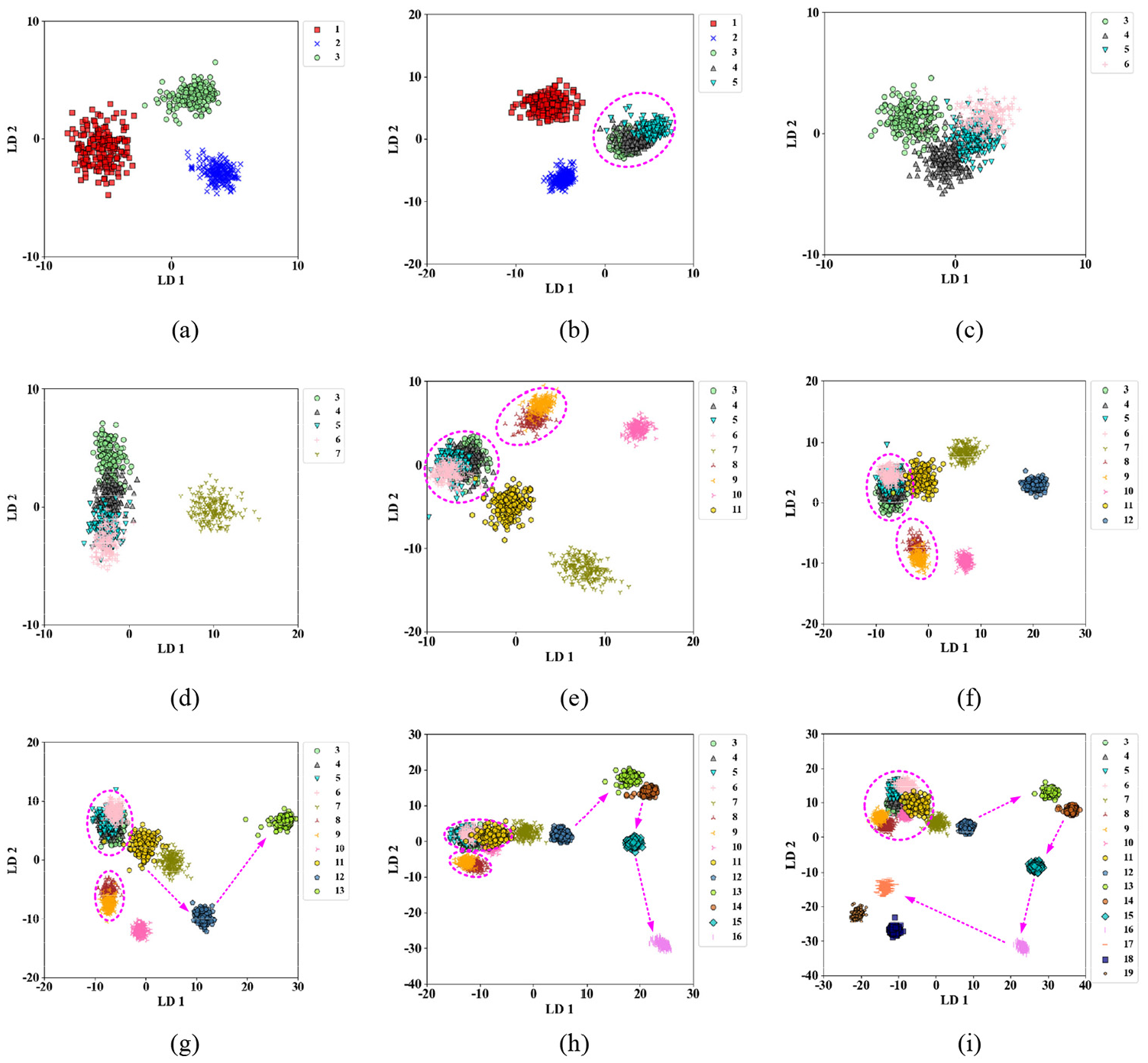
Linear Discriminant Analysis results on the nodes of the first experiment, from (a) to (i) correspond to the 3rd, 5th, 6th, 7th, 11th, 12th, 13th, 16th, 19th node, respectively.

On each node, LDA was restarted and the optimization problem in equation (10) was re-solved on the updated dataset. Each time of LDA was attempted to rediscover a feature space that maximizes class separability based on the updated dataset. The distance of point clouds corresponding to different nodes were informative. And it represented the difference of wheel states on these nodes. In the initial period, samples from the first three nodes can be completely separated as shown in Figure 7(a). It is reasonable because two linear discriminants are sufficient to separate a linearly separable dataset including three classes. When the class number was above three, overlapping was inevitable in two-dimensional feature space. In Figure 7(b), three highly overlapped subsets, which are third and fourth and fifth nodes, are indicated by a dotted circle. A large degree overlap means the insignificant changes of the three nodes compared with the first two ones. Therefore, it can be deduced that the wheel state got a rapid change during the first two nodes and then entered a relatively stable stage from the third node. It coincided with the commonsense that the topography of a new-dressed wheel changes rapidly at the beginning and then stabilizes for the following normal wear stage.³⁸

Only the first two linear discriminants were reserved for visualization, therefore, overlapping was inevitable on the two-dimensional feature space when more than three nodes were involved in LDA. If samples on some history nodes possess quite different characteristics compared with others, LDA will emphasizes the difference and neglects relatively small differences between several of the latest nodes. Moreover, the evolution of wheel state is a typical Markov process,¹⁶ and history states have nothing to do with the future state. Therefore, keeping meaningless history subsets does not help for state discrimination, on the contrary it will blur the difference of the following nodes. Once the wheel entered a stable stage, all sample subsets of history nodes before the stable stage were deleted from the total dataset and didn’t involve in the following analysis. For this reason, on the sixth node, LDA was implemented on the shrunken dataset and the result is shown in Figure 7(c). Even so, samples from the four nodes weren’t separated clearly. It means that wheel state didn’t get a remarkable change from the third to the sixth node. After adding the seventh nodes into LDA, as shown in Figure 7(d), the projection pattern got an obvious change compared with the previous one. The seventh node was far away from others, while all reserved history nodes are entangled with each other. This is due to wheel state got a recognizable change on the seventh node. The difference of the current node from the other ones was overwhelming in LDA, while slight and gradual changes among history nodes from the third to the sixth were further blurred in the newest projection.

Adding the following four nodes after the seventh one by one, the projection pattern didn’t change significantly. In the interest of saving space, only the LDA result on the 11th node is shown in Figure 7(e). The subsets of the eighth and ninth node, which heavily overlapped in the projection, approached the previous stable ones. In LDA, distance manifests the difference of classes. The small distance between the latest two nodes and those stable ones before the seventh node manifested that the wheel state got some recovery after the sudden change on the seventh node. The sudden change probably resulted from self-sharpening of the wheel. Of course, this recovery was limited because there was still a distinct distance between the two stable stages before and after the self-sharpening. Another possible self-sharpening occurred on the 10th node for the 11th node went back to the neighborhood of the nodes in the first stable stage. But the situation was not persistent and soon followed by a more significant transformation. From the 12th node, the current node was more and more far away from stable ones as shown in Figure 7(f) to (i). The degradation process was highlighted by dotted arrows in the plots. According to the LDA results, the wheel should be addressed when the projection of the latest node keeps far away from the stable location. For the wheel used in the first experiment, the 12th node is the proper time point for wheel dressing. According to the topography images on several regions of the wheel, blocking was hard to be recognized even on the next node. Wheel wear can be captured quite early based on AE features. Moreover, exactly capturing illegible early blocking is unlikely in practice because of the limitation of detection range and accuracy of image detection. By contrast, AE feature is more sensitive and suitable for early warning of the degradation of wheel condition.

The case of the second experiment is shown in Figure 8. Dotted purple lines and circles assist to recognize the change of projection pattern. Originally separating subsets in Figure 8(a) arrange in a line in Figure 8(b) when the fourth node involved in the LDA. It means that wheel state on the fourth node was quite different from the previous ones which made the linear discriminants dramatically changed. Next, the comparison between Figure 8(b) and Figure 8(c) shows that the relative positions of the first three nodes were basically fixed when continuing add the fifth and sixth node. Data samples naturally assembled in two clusters which are strung by two purple curves in Figure 8(c). The projection pattern got a slight change after adding the fifth and sixth node. LDA emphasized the difference between the two clusters. The fourth node can be taken as a watershed node for the evolution of wheel state. Considering the wheel was just after dressing, the first three nodes were classified into the early wear stage.

Figure 8.

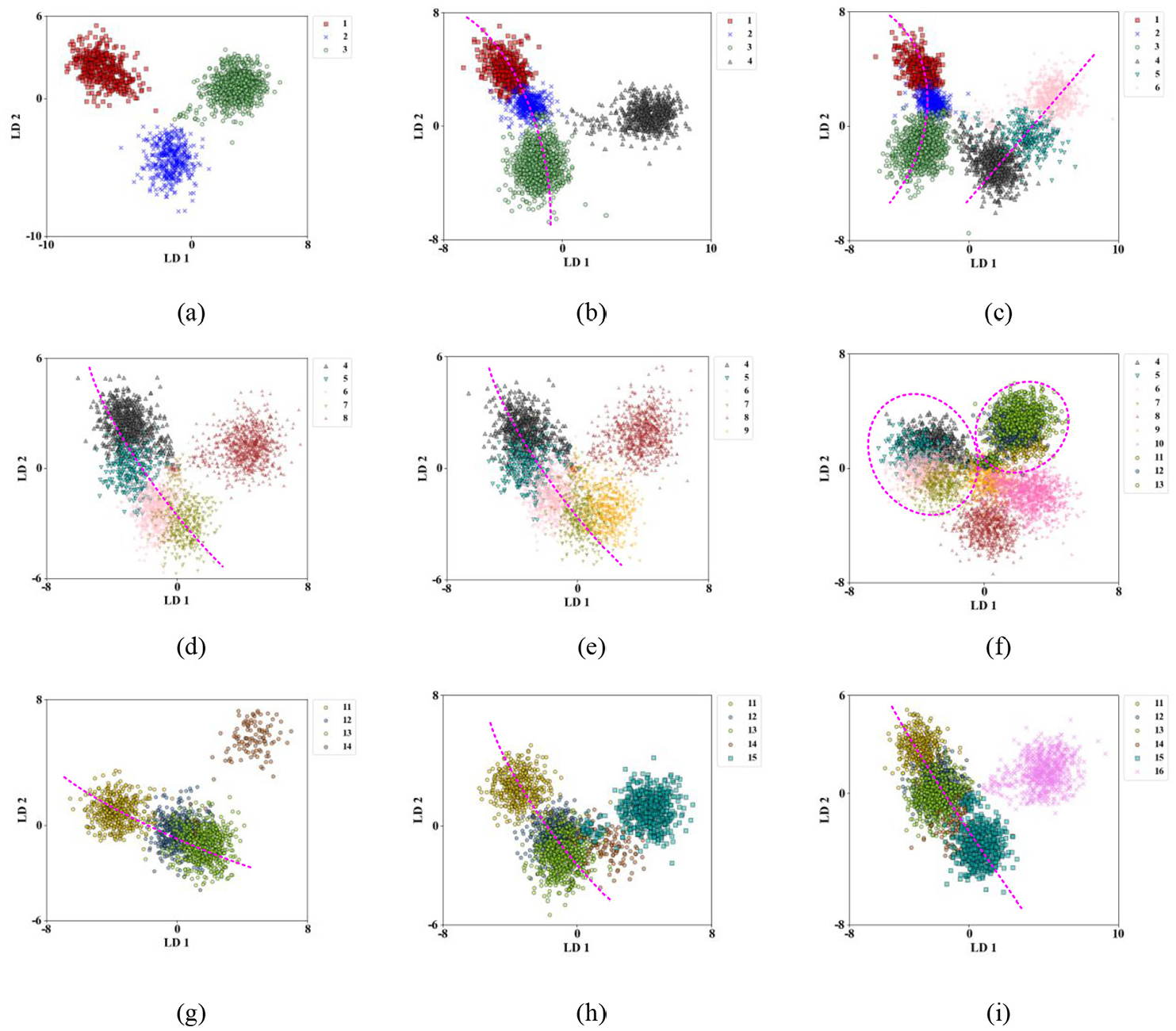
Linear Discriminant Analysis results on the nodes of the second experiment, from (a) to (i) correspond to the 3rd, 4th, 6th, 7th, 8th, 12th, 13th, 15th, 16th node, respectively.

For the same reason mentioned in the first experiment analysis, samples of the early wear stage were removed from the dataset for the following LDA. As shown in Figure 8(d), the subset of the eighth node is separated from the others, which means the wheel state got an obvious change on the eighth node. After that, the optimal projection direction was almost unchanged when the ninth node involved. Basically, the subsets of fourth to seventh are successively arranged in a ray in Figure 8(d), and so is the same in Figure 8(e). The 9th node basically followed the direction of the ray and the sample point cloud of the ninth node significantly superimposed on the seventh. It means that wheel state on the 9th node was more similar to the state before the eighth. Therefore, the eighth node was identified as self-sharpening of the wheel. Another self-sharpening was identified on the 10th node as shown in Figure 8(f). After adding the subset of the 10th node into LDA, the subsets of fourth to seventh, which were originally arranged in a line as shown Figure 8(e), clustered together in Figure 8(f). Significant overlap manifested stability of wheel state. Therefore, they can be recognized as a stable stage. The involvement of the next three nodes (the 11th–13th) got a slight change in the projection, and they were also cluster together in Figure 8(f). Therefore, the 11th to 13th was another stable stage of wheel state. Two stable stages are marked by ellipses on the projection. Because of the incomplete recovery of wheel state after self-sharpening, point clouds of the two stable stages were separated clearly.

As suggested before, once a wheel enters a stable stage, all history subsets before the stable stage are excluded from the following LDA. The LDA results on the next three nodes are shown in Figure 8(g) to (i), respectively. The optimal projection direction was constantly changing with the successive involvement of the three nodes, which means a rapid development for the wheel state. The 16th node was the last one before the workpiece was broken. Considering almost the same topography of the wheel before and after the break, AE-based monitoring are more suitable for early warning. The straight wheel underwent several times of self-sharpening and stayed in subsequently stable stages. Frequently self-sharpening meaned the continuous decline of grinding performance of the wheel. It was a sign for wheel dressing.

Discussion

Experimental results of two commonly used diamond wheels have been detailed analyzed in the previous section. Although the evolvement of wheel state can be accurately traced for both wheels, there were something difference for the judgment. In the first experiment, distinct distance existed between different stages. But for the straight wheel used in the second experiment, there was not significantly distance between them. Decision-making basically relied on the change of the projection pattern. The difference resulted from the diversity of spectra of AE samples. Observing AE spectra in Figures 5 and 6 shows that spectra possessed identifiable difference in amplitude and energy distribution for the cup wheel, while there were quite similar spectra during the whole life cycle of the straight wheel. Therefore, locations of all subsets on the projection are close even for those lie in different stages. Wheel topography also gives clues for the different representation of the two wheels. As shown in Figures 3 and 4, the change of the topography of the cup wheel is recognizable during the rear part of the process. However, the straight wheel almost kept the topography after the early wear stage.

No matter slight or unexplainable complex changes in AE spectra, LDA highlights the difference of AE samples and employs the relative changes of adjacent sample subsets to judge the successive changes of wheel state. Different from model-based wheel condition monitoring methods with fixed wear stage division, the proposed method is adaptable and identifies detailed stages according to the actual development of wheel state. It is a robust online monitoring method which is adaptable for different grinding technologies and wheel wear types.

Conclusions

In this paper, a universal method of tracking state evolution of diamond wheel during grinding brittle materials is proposed based on AE signals. The separation and superposition characteristics of AE components with various mechanisms in frequency domain make AE spectra suitable for feature representation. Linear Discriminant Analysis was used to project spectra of time-ordered AE samples into a two-dimensional feature space and the transformation of wheel state can be deduced by observing the changes of the projection.

Two types of commonly used diamond wheels for optical surface grinding, which are straight wheel and cup wheel, were used to verify the accuracy of the proposed monitoring strategy. Life cycle experiments were carried out on two grinding machines. The degradation and recovery of wheel condition can be captured precisely and timely, no matter what kind of wear types they were. Generally speaking, the recovery of wheel condition by self-sharpening is limited. To insure the consistent wheel condition during precision grinding of optical components, frequently self-sharpening is a sign of down-time for wheel dressing.

Employing the time sequence of AE samples during grinding process, the proposed monitoring strategy focused solely on change intensity of wheel state and avoided delicate sample labeling and complex model training. Therefore, it is a universal method and easy to be implemented in practice. During grinding optical components, the final purpose of wheel state monitoring is to avoid catastrophic damages on or beneath the ground surface. Considering the close relationship between AE signals and fracture mechanisms, further work will focus on the prediction and suppression subsurface damage depth of large scale optical components. Diverse AE mechanisms under grinding brittle materials will be paid more attention to in order to reveal the correlation of AE features and subsurface damages.

Footnotes

Appendix

Declaration of conflicting interests

The author(s) declared no potential conflicts of interest with respect to the research, authorship, and/or publication of this article.

Funding

The author(s) disclosed receipt of the following financial support for the research, authorship, and/or publication of this article: This work was funded by National Natural Science Foundation of China (No. 51805459).

ORCID iD

Bi Guo

References

Oliveira

Silva

Guo

, et al. Industrial challenges in grinding. CIRP Ann Manuf Technol 2009; 58: 663–680.

Brinksmeier

Heinzel

Meyer

Development and application of a wheel based process monitoring system in grinding. CIRP Ann Manuf Technol 2005; 54: 301–304.

Davies

Ueda

M’Saoubi

, et al. On the measurement of temperature in material removal processes. CIRP Ann Manuf Technol 2007; 56: 581–604.

Wegener

Hoffmeister

Karpuschewski

, et al. Conditioning and monitoring of grinding wheels. CIRP Ann Manuf Technol 2011; 60: 757–777.

Lee

SH.

Analysis of ductile mode and brittle transition of AFM nanomachining of silicon. Int J Mach Tools Manuf 2012; 61: 71–79.

Inasaki

Application of acoustic emission sensor for monitoring machining processes. Ultrasonics 1998; 36: 273–281.

Liang

Hecker

Landers

RG.

Machining process monitoring and control: the state-of-the-art. J Manuf Sci Eng 2004; 126: 297–310.

Sutowski

Plichta

An investigation of the grinding wheel wear with the use of root-mean-square value of acoustic emission. Arch Civil Mech Eng 2006; 6: 87–98.

Strantza

Van Hemelrijck

Guillaume

, et al. Acoustic emission monitoring of crack propagation in additively manufactured and conventional titanium components. Mech Res Commun 2017; 84: 8–13.

10.

Mokbel

Maksoud

TM.

Monitoring of the condition of diamond grinding wheels using acoustic emission technique. J Mater Process Technol 2000; 101: 292–297.

11.

Chai

Zhang

Duan

A new qualitative acoustic emission parameter based on Shannon’s entropy for damage monitoring. Mech Syst Signal Process 2018; 100: 617–629.

12.

Lopes

Junior

POC

Aguiar

, et al. An efficient short-time Fourier transform algorithm for grinding wheel condition monitoring through acoustic emission. Int J Adv Manuf Technol 2021; 113: 585–603.

13.

Chen

Griffin

Liu

Mechanical and thermal behaviours of grinding acoustic emission. Int J Manuf Technol Manag 2007; 12: 184–199.

14.

Yang

Xie

, et al. Application of Hilbert–Huang transform to acoustic emission signal for burn feature extraction in surface grinding process. Measurement 2014; 47: 14–21.

15.

Liang

SY.

A critical energy model for brittle–ductile transition in grinding considering wheel speed and chip thickness effects. Proc IMechE, Part B: J Engineering Manufacture 2016; 230: 1372–1380.

16.

Liao

TW.

Feature extraction and selection from acoustic emission signals with an application in grinding wheel condition monitoring. Eng Appl Artif Intell 2010; 23: 74–84.

17.

Lezanski

An intelligent system for grinding wheel condition monitoring. J Mater Process Technol 2001; 109: 258–263.

18.

Nakai

Aguiar

Guillardi

, et al. Evaluation of neural models applied to the estimation of tool wear in the grinding of advanced ceramics. Expert Syst Appl 2015; 42: 7026–7035.

19.

Krishnan

Rameshkumar

Grinding wheel condition prediction with discrete hidden Markov model using acoustic emission signature. Mater Today Proc 2021; 46: 9168–9175.

20.

Liao

Tang

, et al. Grinding wheel condition monitoring with boosted minimum distance classifiers. Mech Syst Signal Process 2008; 22: 217–232.

21.

Lee

Jwo

Hsieh

, et al. An intelligent system for grinding wheel condition monitoring based on machining sound and deep learning. IEEE Access 2020; 8: 58279–58289.

22.

Guo

Zhou

QZ.

An intelligent monitoring system of grinding wheel wear based on two-stage feature selection and long short-term memory network. Proc IMechE, Part B: J Engineering Manufacture 2019; 233: 2436–2446.

23.

Lin

Wang

Jiang

, et al. Online force control of large optical grinding machine for brittle materials assisted by force prediction. Proc IMechE, Part B: J Engineering Manufacture 2020; 234: 14–26.

24.

Neauport

Ambard

Cormont

, et al. Subsurface damage measurement of ground fused silica parts by HF etching techniques. Opt Express 2009; 17: 20448–20456.

25.

Zhao

Liang

Stephenson

, et al. Surface and subsurface integrity in diamond grinding of optical glasses on Tetraform ‘C’. Int J Mach Tools Manuf 2007; 47: 2091–2097.

26.

Palmer

Curtis

Novovic

, et al. The influence of abrasive grit morphology on wheel topography and grinding performance. Procedia CIRP 2018; 77: 239–242.

27.

XL.

A brief review: acoustic emission method for tool wear monitoring during turning. Int J Mach Tools Manuf 2002; 42: 157–165.

28.

. Research on processing & characterization and experiment of acoustic emission signal in diamond tool grinding. Dissertation. Harbin Institute of Technology, China, 2015.

29.

Wisner

Mazur

Perumal

, et al. Acoustic emission signal processing framework to identify fracture in aluminum alloys. Eng Fract Mech 2019; 210: 367–380.

30.

Kharrat

Placet

Ramasso

, et al. Influence of damage accumulation under fatigue loading on the AE-based health assessment of composite materials: wave distortion and AE-features evolution as a function of damage level. Compos A Appl Sci 2018; 109: 615–627.

31.

Resendiz-Ochoa

Saucedo-Dorantes

Benitez-Rangel

, et al. Novel methodology for condition monitoring of gear wear using supervised learning and infrared thermography. Appl Sci 2020; 10: 506.

32.

Tan

Luan

, et al. 2DPCA versus PCA for face recognition. J Central South Univ 2015; 22: 1809–1816.

33.

Yuan

2D-LDA: a statistical linear discriminant analysis for image matrix. Pattern Recognit Lett 2005; 26: 527–532.

34.

Liu

, et al. Diamond grinding wheel condition monitoring based on acoustic emission signals. Sensors 2021; 21: 1054.

35.

Martinez

Kak

AC.

PCA versus LDA. IEEE Trans Pattern Anal 2001; 23(2): 28–233.

36.

Webb

AR.

Statistical pattern recognition. 2nd ed. West Sussex: John Wiley & Sons, Ltd, 2003.

37.

Pedregosa

Varoquaux

Gramfort

, et al. Scikit-Learn: machine learning in Python. J Mach Learn Res 2011; 12: 2825–2830.

38.

Rowe

WB.

Principles of modern grinding technology. 2nd ed. Waltham, MA: William Andrew, 2014.

Tracking changes in grinding wheel condition using reduced features of acoustic emission signals

Abstract

Keywords

Introduction

Basic theory

Characteristics of AE signals in frequency domain

Dimensionality reduction of AE spectrum based on LDA

Monitoring strategy for wheel state evolution

Experiments

Experimental instruments and parameters

Wheel wear monitoring by reduced dimensional features of AE signals

Discussion

Conclusions

Footnotes

Appendix

Declaration of conflicting interests

Funding

ORCID iD

References