Sage Journals: Discover world-class research

Abstract

Welding quality inspection is critical to the quality control of the welding structure. Traditional manual detection requires experienced workers and the method is time-consuming. Currently, deep learning has made great progress in the field of image recognition. However, in terms of industrial defect detection, the contradiction between huge computational parameters and limited imbalanced samples still exists, which makes the deep learning method unable to play its role to the maximum extent. In this case, a combination of deep learning methods and transfer learning methods is considered to improve the performance of the model on limited and imbalanced data sets. The VGG16 model, which is pre-trained on a large number of source data sets, is fine-tuned on our target data sets. In this paper, a new DTN-VGG16 structure is proposed, in which a Global Average Pooling (GAP) layer, Batch Normalization (BN) layer, and Soft-max classifier are added on top of the frozen pre-training model, which can effectively reduce the number of parameters and accelerate the convergence speed of the model. In addition, focal loss function is used to replace the commonly used multi-class cross entropy loss function. By adjusting the parameters of the loss function, the training process has better convergence. Experimental results show that DTN-VGG16 has better performance than other traditional machine learning methods and deep learning models. And the proposed model has good robustness and generalization performance when valid on the real data of aerospace welding seams which is difficult to learn.

Keywords

Weld defect identification deep learning transfer learning small sample imbalanced dataset

Introduction

The connection between metals usually adopts the welding method. In order to ensure that the strength of welding parts meet the requirements, it is necessary to check the quality of welding seam. Weld quality inspection is important to ensure the safety and reliability in the industrial field, especially in aerospace, shipbuilding, railway, and pipeline construction.¹ Nondestructive Testing (NDT) is a common welding detection method, which mainly includes visual inspection, penetrant, magnetic powder, ultrasonic, and radiography. And radiography (X-ray) detection is one of the most widely used and widely accepted welding detection methods.² In the field of aeronautics, X-ray detection is mostly used to detect the weld quality. This method can photograph the internal welding state that cannot be seen by human eyes.³

Early defect classification methods mainly extracted features of defect images manually or through algorithms, and then input feature sets into some traditional machine learning classifiers, such as support vector machine (SVM)⁴ and artificial neural network (ANN).⁵ For example, a three-step defect detection method was proposed, in which the wavelet de-noising method was used to process the ray images.⁶ In the paper of Kumar et al.,⁷ the author used adaptive Wiener filter to reduce noise, and applied contrast enhancement technology to implement image preprocessing steps. Valavanis and Kosmopoulos proposed a method of multiclass defect detection based on feature selection and classification system, selected the attributes of geometry and texture feature which on behalf of the image as input, SVM, and ANN as classifiers to classify the defect types. They proved that good feature selection can significantly reduce the computational time without a significant reduction in classification accuracy.⁸ However, these methods need to be manually operated and supported by the professional knowledge of the workers.

Deep learning method, especially convolutional neural network (CNN), has performed well in image recognition and can automatically learn image features. This method has been successfully applied to many defect detection projects and has shown excellent performance. Most of these network models are based on the classical convolutional neural network, which can combine the operations of feature extraction and classification into one model to classify the defect images.^9,10 Hou et al.¹¹ cut out images of 32 × 32 size from theX-ray images of welds for binary classification of defects based on the deep neural network. After training, the model was applied to the defect classification of the whole picture, and the defect areas were marked by threshold judgment. Liu et al.¹² proposed a full convolutional network based on VGG16 to classify weld defect images of different sizes, which achieved high accuracy on a relatively small data set. It can not only automatically extract image features, but also have high classification accuracy. Deep convolutional neural network (DCNN) model proposed by Hou et al.¹³ proved that the deep features learned by deep learning networks are more separable than traditional features.

Transfer learning can use the model previously trained on a larger data set as knowledge to be transferred to the data set with a smaller sample size for training. Transfer learning has been applied in many fields, such as medical image analysis,¹⁴ diagnostic assessment of machine health,¹⁵ surface defect detection,¹⁶ and so on. For example, Zheng et al.¹⁷ used the convolutional layer feature of VGGNet to locate and distinguish images. Gopalakrishnan et al.¹⁸ used convolution blocks of VGG16 as feature extractor, and then replaced the final full connection layer with some traditional machine learning classifiers, which achieves a good effect on road defect images. But the classification accuracy still needs to be improved. The TL-Mobilenet model proposed by Pan et al.¹⁹ achieved an accuracy rate of 97.69% in the weld image data, but the method was still based on the classification of large balanced data sets, while in the actual situation, the defect categories was imbalanced.

At present, most relevant researches are based on model experiments of a large number of public data sets, and there are not enough researches on image classification of weld defects. The reality of the industry is that target data is scarce and some defect types have never been seen before in history. All this will affect the classification process. To solve the above problems, we proposed a transfer learning model based on CNN to solve the problem of welding seam defect image classification. By comparing our method with those convolutional neural networks based on other backbones, the experiment proves that our method can achieve the highest accuracy and the lowest loss, and performs well in the validation data set. At the same time, good results are obtained on both public datasets and real industrial datasets, indicating the effectiveness and robustness of our method.

Model architecture and performance metrics

Architecture of the proposed model

The fine-tuning method of the model is generally to train the data set by freezing the previous feature extraction layer and changing the last layer or some layers. This can save time to some extent and solve the problem of small sample learning. Many transfer learning networks freeze the convolution blocks as the feature extraction layer and then train the final full connection layer classifier. However, the full connection layer usually accounts for the majority of the network model parameters. Therefore, our model use the VGG16 network model trained on the ImageNet public data set as the foundation. In order to improve the convergence speed of the model, a Batch Normalization layer was added, followed by ReLU activation function. Then a Global Average Pooling layer and a soft-max classification layer were added to build a new DTN-VGG16 model. GAP does not need a lot of training tuning parameters, reducing the spatial parameters will make the model more robust, to prevent overfitting.

At the same time, the several convolution layers in front of the feature extraction layer are mostly to extract the features of some obvious regions, such as edge information, etc., which has little difference in layer parameters among different images. Therefore, we only choose to defrost the fifth convolution block, keep the previous convolutional blocks frozen, and use a smaller learning rate to retrain the network and learn deeper information. The architecture of our model is shown in Figure 1.

Figure 1.

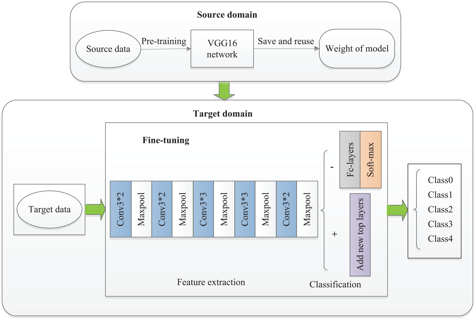
Architecture of the proposed DTN-VGG16 classification model.

Performance metrics

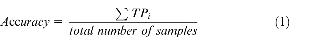
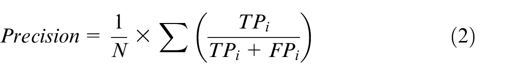
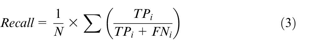
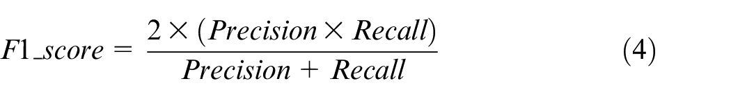
Since the model is aimed at the classification of imbalanced and small sample data, in addition to classification accuracy, we need to consider more indicators such as precision, recall, and F1-score. Macro average rule is considered to calculate the precision and recall, that is to calculate the precision and the recall for categories, and finally to calculate the overall average value. The relevant formulas are shown as below.

A cc uracy = \frac{\sum T P_{i}}{total number of samples}

(1)

Precision = \frac{1}{N} \times \sum (\frac{T P_{i}}{T P_{i} + F P_{i}})

(2)

Recall = \frac{1}{N} \times \sum (\frac{T P_{i}}{T P_{i} + F N_{i}})

(3)

where $i$ represents category, $N$ represents the total number of categories. $T P_{i}$ represents the number of samples that its predicted value is category $i$ and the predicted value is correct, $F P_{i}$ represents the number of sample that its predicted value is category $i$ but the predicted value is wrong. And $F N_{i}$ represents the number of samples that its true label is category $i$ but the predicted value is wrong.

F 1_score = \frac{2 \times (Precision \times Recall)}{Precision + Recall}

(4)

In addition, to make the model results more intuitive, we also chose to visualize the final results by the confusion matrix and the receiver operating characteristic (ROC) curve.

Data description

Images used for classification experiment from GDXray public database, which includes five sets of ray images including Castings, Welds, Baggage, Nature, and Settings.²⁰ The data set of Welds, with a total of 88 image data. Among them, 10 images with pixel-wise ground truth. One of the images with its pixel-wise ground truth is shown in Figure 2.

Figure 2.

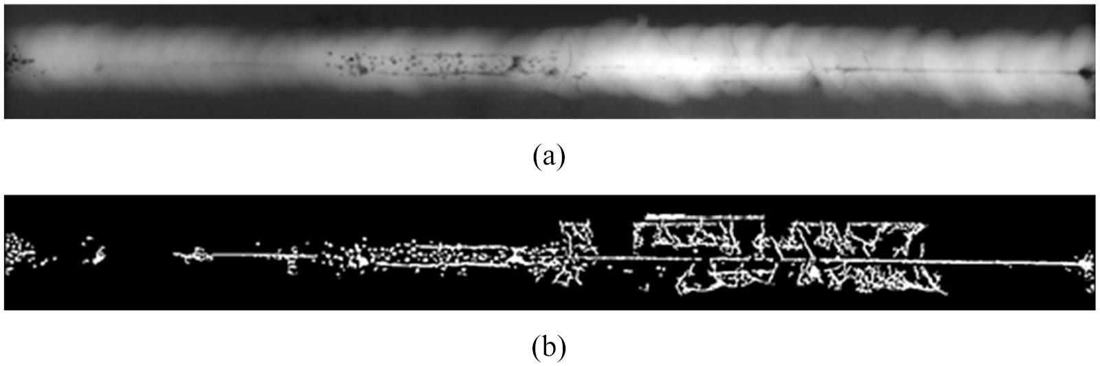
An image sample of welds in GDXray data set: (a) grayscale images of weld defects and (b) pixel-wise ground truth of weld defects.

According to the characteristics of the image data, appropriate method needed to be chosen to augment images. In this paper, the sliding window method was selected to crop the image. The window size was set to 224 × 224 and the step size was set to 100. The process of image acquisition is shown in Figure 3.

Figure 3.

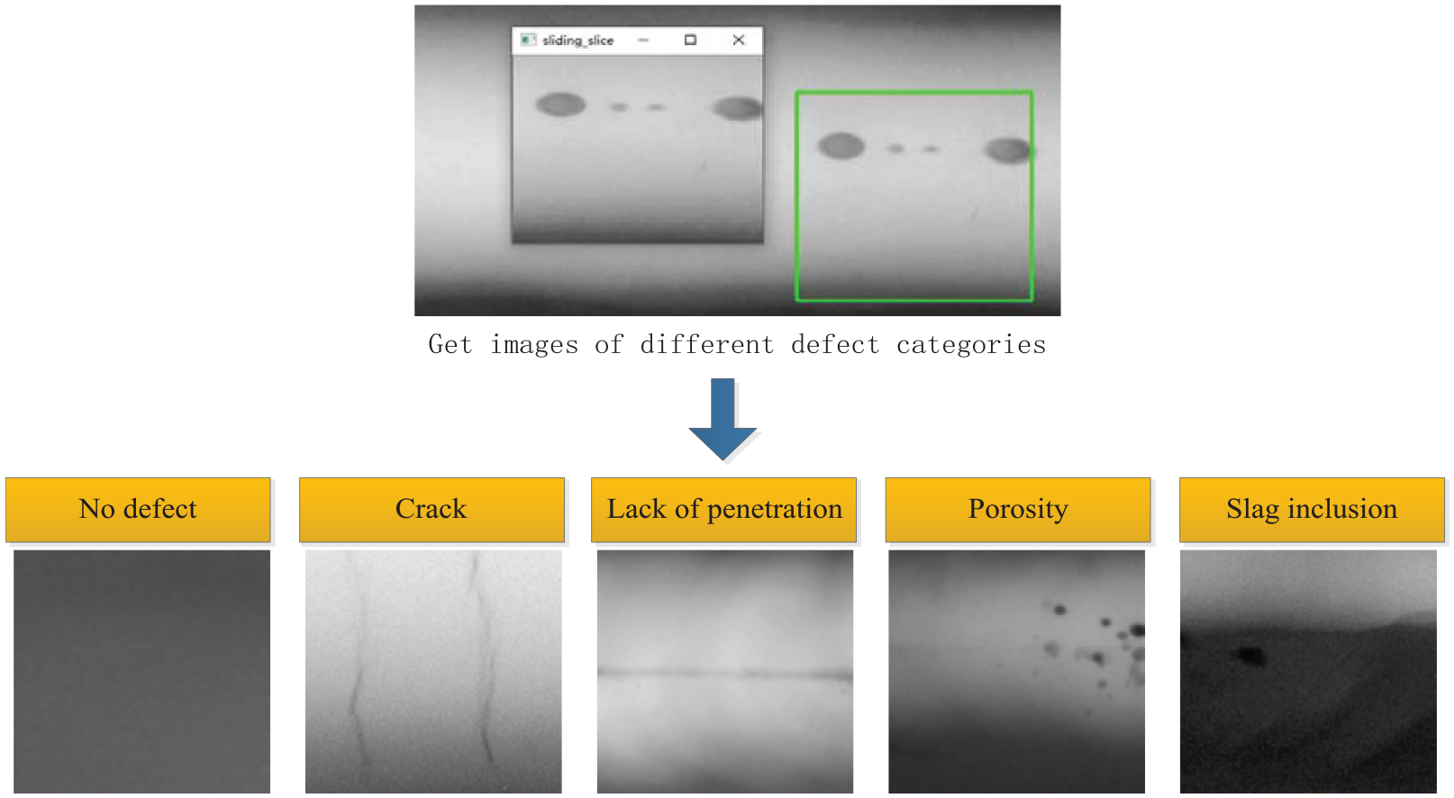
Weld defects dataset obtained by sliding window cropping method.

A total of 2018 images were obtained initially through cropping. Among them, 1428 pictures are no defects (ND), 140 pictures with cracks (CK), 201 pictures with lack of penetration (LOP), 168 pictures with porosity (PO), and 81 pictures with slag inclusion (SI). As shown in the Figure 4. There is a big difference between the number of the majority images and the number of the minority images.

Figure 4.

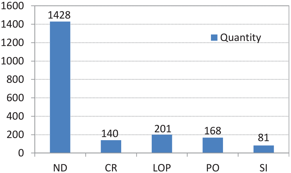
The quantity distribution of weld defects dataset.

Experiments

Parameters of focal loss function

The initial image samples are limited and imbalanced. This kind of situation will make the deep learning model tend to learn the majority of categories, which will greatly reduce the classification effect of the final model. The direction of improvement is generally divided into data level, algorithm level and the combination method of data and algorithms.

Data level: Generally, over-sampling (interpolation) and under-sampling (compression) are used to eliminate the imbalance to a certain extent. Methods for data generation such as: the synthetic minority oversampling technique (SMOTE),²¹ GAN.

Algorithm level: It mainly improves the existing deep learning algorithm and eliminates the influence of category imbalance by modifying the loss function or learning method. The loss functions used for imbalanced images classification include: focal loss,²² dice loss, and so on.²³

Ensemble Methods: The ensemble method of data and algorithms is to consider both the data level and the algorithm level.

We choose focal loss function to solve the problem of category imbalance. Based on the traditional cross entropy loss function, focal loss function adds category weight and modulating factor of sample difficulty weight to alleviate the imbalance problem of sample categories and sample classification difficulty, which will make the classification result more accurate. The formula of focal loss function is as follows:

FL = - alpha {(1 - p_{t})}^{gamma} \log (p_{t})

(5)

where $p_{t}$ is the probability that a certain type of prediction result is correct, alpha can be used to adjust the weight of all categories, and gamma can be used to adjust the loss of difficult and easy training samples.

Generally, a lower weight is set for the majority of samples, and a larger weight is set for the minority of samples, so as to reduce the loss of the majority of samples and increase the loss of the minority of samples. In this paper, alpha = [0.25, 0.9, 0.9, 0.9, 0.9]. Gamma can improve the loss of difficult training samples, and reduce the loss of easy training samples. In this paper, gamma = 2.

We compared the training results of using cross entropy loss function and focal loss function respectively. It can be seen from Figure 5 that although the focal loss function did not significantly improve the accuracy of the model, it alleviated the shock of the curve of training process to a large extent and made the model converge faster.

Figure 5.

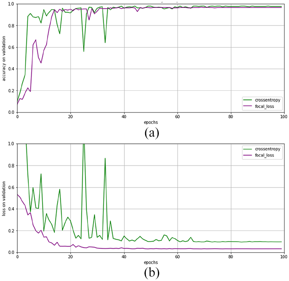
The performance of different loss functions on the validation set: (a) the accuracy of the two loss functions on the verification set and (b) the loss of the two loss functions on the verification set.

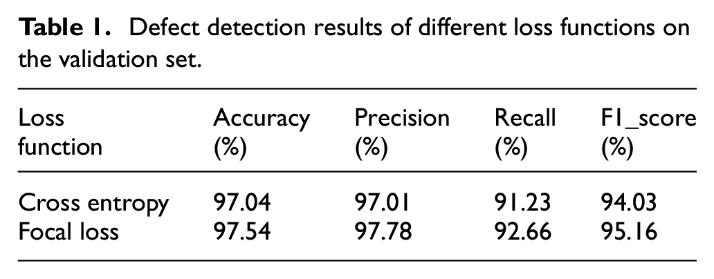
Finally, the predicted results of the two different loss functions on the test set are shown as Table 1. The focal loss function can improve the performance of the model compared with cross entropy loss function. It can be seen from Table 2 that although the overall recall rate reaches 92.66% while using focal loss function, the recall rate of three types of defects is less than 90%.

Table 1.

Defect detection results of different loss functions on the validation set.

Lossfunction	Accuracy(%)	Precision(%)	Recall(%)	F1_score(%)
Cross entropy	97.04	97.01	91.23	94.03
Focal loss	97.54	97.78	92.66	95.16

Table 2.

Recall rates of different types using focal loss function.

Defect type	ND	CR	LOP	PO	SI	Recall (%)
ND	286	0	0	0	91.23	100.00
CR	2	25	1	0	0	89.29
LOP	0	0	40	1	0	97.56
PO	4	0	0	30	0	88.24
SI	1	0	0	1	5	88.24

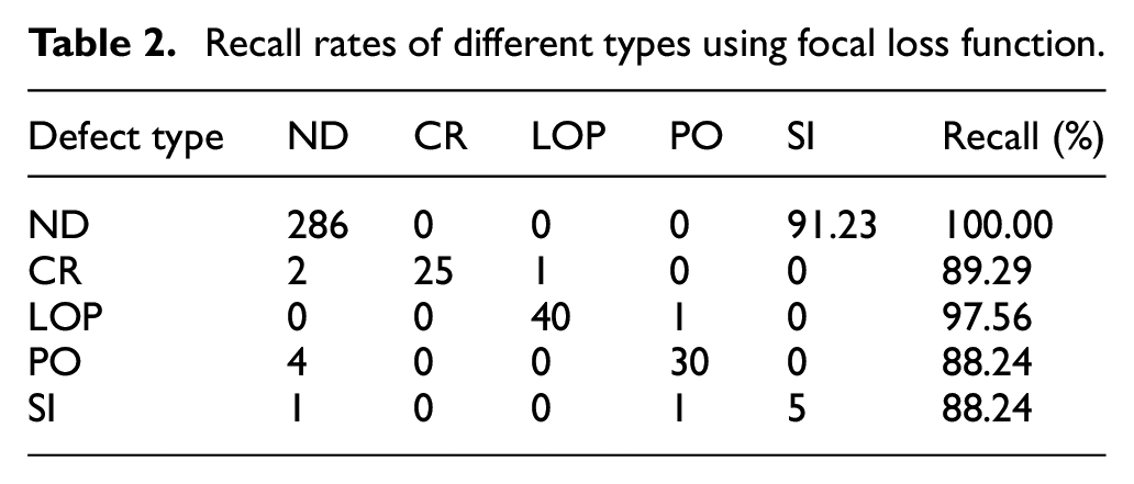
Therefore, we still need to improve the performance of the model from the data level. We oversampled the minority of categories, copied several defect images from these categories, clipped them, and added them to their corresponding defect categories. And we also removed some of the low quality images from them. After the operation of the data level, and ultimately our overall sample data sets reached 2189 pieces, among them the defect categories and their corresponding images quantity is {ND: 1427, CR: 196, LOP: 199, PO: 197, SI: 170}.

Data partition and final parameters setting

The data set was divided into training set and test set according to the ratio of 8:2. In the process of model training, a 5-Fold cross validation was carried out on the training set, as shown in Figure 6. And the average validation accuracy, validation loss, and their corresponding standard deviation (Std) were used to evaluate the performance of the model on the training set. Finally, the selected optimal model was tested on the test set to evaluate the generalization performance of the model.

Figure 6.

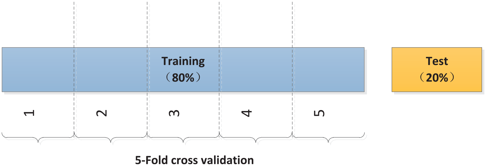
Divide the training and testing with ratio of 8:2.

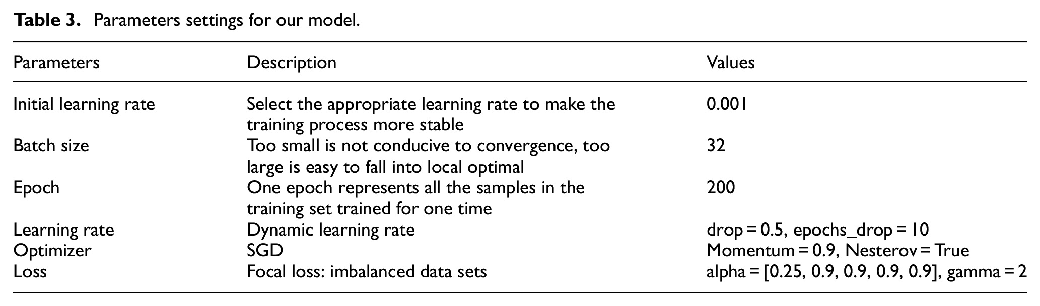
It should be noted that since our model has been trained on the large data set before, it has acquired certain feature extraction capability. If the initial learning rate is set too high, the model training curve will shake obviously. Therefore, the learning rate can be appropriately reduced during the training process. In this experiment, we set the initial learning rate to 0.001. And adopt the learning rate dynamic adjustment strategy of step attenuation. The formula of learning rate is as follows:

lr = initial_lr \times dro p^{floor (epoch / epochs_drop)}

(6)

The formula (6) shows that the final learning rate which is based on the initial learning rate, will decays with a certain number of epochs according to the decay factor. The experimental programming environment is based on Python 3.7, using Keras framework with TensorFlow as the backend. Some of the specific parameter settings are shown in Table 3.

Table 3.

Parameters settings for our model.

Parameters	Description	Values
Initial learning rate	Select the appropriate learning rate to make the training process more stable	0.001
Batch size	Too small is not conducive to convergence, too large is easy to fall into local optimal	32
Epoch	One epoch represents all the samples in thetraining set trained for one time	200
Learning rate	Dynamic learning rate	drop = 0.5, epochs_drop = 10
Optimizer	SGD	Momentum = 0.9, Nesterov = True
Loss	Focal loss: imbalanced data sets	alpha = [0.25, 0.9, 0.9, 0.9, 0.9], gamma = 2

Comparison results of different backbone networks

The performance of our model is compared with that of some other classical models with different input size. The input size includes five types, which are 48 × 48,96 × 96, 144 × 144, 192 × 192, 224 × 224. It is worth noting that there are limitations about the input size of different model, such as the Xception network and the InceptionV3 networks, which require input sizes of M > 71 and M > 75 respectively. Because when the input size is too small, the feature maps obtained by the model will be less than 3 × 3, which will affect the learning process of the model. Dynamic learning rate adjustment strategy and focal loss function were adopted in all models, and the parameters are set the same as in Table 3. Finally, the 5-fold cross validation is carried out to obtain the average accuracy, average loss, and their corresponding standard deviation (Std) of each model. The comparative experimental results are shown in Table 4.

Table 4.

Comparison results of different backbone network with different input sizes..

Size (M × M)	Mean	Xception	InceptionV3	ResNet-50	VGG19	Ours
M = 48	Accuracy (%) (Std)	M > 71	M > 75	78.50% (8.02%)	96.85% (0.85%)	97.54% (0.97%)
	Loss (Std)			0.2035 (0.0614)	0.0330 (0.0111)	0.0272 (0.0135)
M = 96	Accuracy (%) (Std)	96.91% (1.44%)	93.37% (1.16%)	88.79% (3.91%)	97.48% (0.95%)	98.14% (0.94%)
	Loss (Std)	0.0296 (0.0116)	0.0782 (0.0237)	0.0790 (0.0179)	0.0235 (0.0113)	0.0201 (0.0084)
M = 144	Accuracy (%) (Std)	97.66% (0.49%)	96.85% (0.94%)	88.68% (2.18%)	97.43% (0.65%)	97.60% (0.59%)
	Loss (Std)	0.0231 (0.0063)	0.0426 (0.0148)	0.1044 (0.0180)	0.0285 (0.0127)	0.0236 (0.0106)
M = 192	Accuracy (%) (Std)	97.54% (1.04%)	97.31% (0.99%)	91.31% (1.49%)	96.68% (1.34%)	96.68% (0.84%)
	Loss (Std)	0.0267 (0.0081)	0.0334 (0.0141)	0.0885 (0.0160)	0.0342 (0.0143)	0.0303 (0.0128)
M = 224	Accuracy (%) (Std)	97.14% (0.99%)	97.48% (1.27%)	91.71% (1.57%)	96.28% (1.11%)	96.51% (0.96%)
	Loss (Std)	0.0289 (0.0083)	0.0317 (0.0152)	0.0853 (0.0129)	0.0384 (0.0140)	0.0349 (0.0138)
Running time of the optimal model		16 min 47 s	22 min 22 s	23 min 20 s	11 min 39 s	11 min 17 s

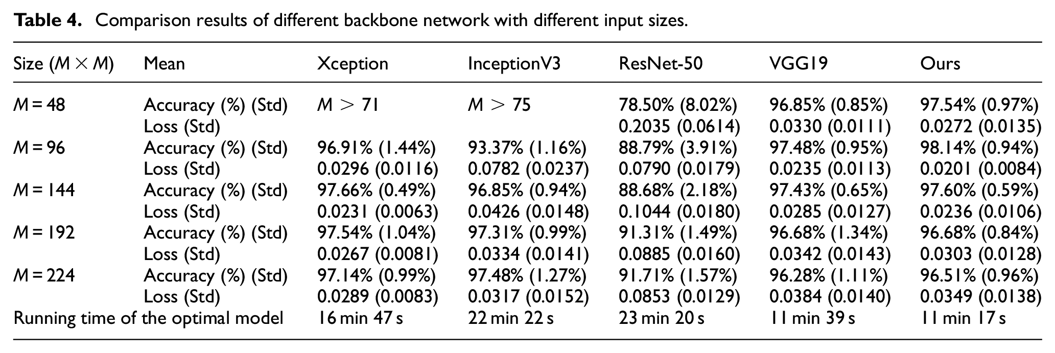
As can be seen from Table 4, our model is superior to other models in accuracy performance and loss performance, reaching 98.00%and 0.0201 respectively. Xception achieved the highest accuracy of 97.66% when the input size was 144 × 144, and InceptionV3 achieved the highest accuracy of 97.48% when the input size was 224 × 224. However, as the input size becomes larger, the training parameters increase and the running time of the model is longer. According to the average running time (epoch = 200) of the optimal models with different input sizes, the proposed model is the fastest, requiring only 11 min 17 s. Considering the accuracy and running time, the proposed model in this paper has better performance.

To some extent, the size of the input image will affect the prediction accuracy and loss of the model. In a certain range, the larger the image size is, the more information the feature map obtained by the model contains, which is beneficial to the learning process of the model. Otherwise, as the input size increases, the resolution of the image may decrease (resolution × size of the image = pixels), blurring the image and affecting classification accuracy and loss performance. In short, the optimal input size still needs to be determined through the experiment.

Final classification result

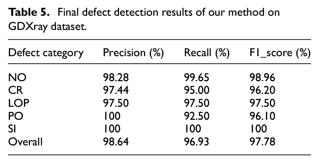
Our model was retrained when the input size was 96 × 96 and tested on the test set. The final test accuracy of the model is 98.41%. The precision, recall, and F1_score of various categories are shown as Table 5.

Table 5.

Final defect detection results of our method on GDXray dataset.

Defect category	Precision (%)	Recall (%)	F1_score (%)
NO	98.28	99.65	98.96
CR	97.44	95.00	96.20
LOP	97.50	97.50	97.50
PO	100	92.50	96.10
SI	100	100	100
Overall	98.64	96.93	97.78

As can be seen from the confusion matrix in Figure 7, the classification recognition rate of our model is very high, and the performance of recall rate is greatly improved compared with the Table 1. Especially for the category of SI defect, the recall rate reaches 100% although the number of samples is the lowest. However, there are still have a small amount of misclassification, By finding out these misclassified images, we found that these images have one thing in common, that is, the defect area is not obvious, and the defect area takes up a very small area in the whole picture. After operations such as convolution and pooling, sufficient characteristic information cannot be obtained, which makes the model tend to determine these categories as having no defects.

Figure 7.

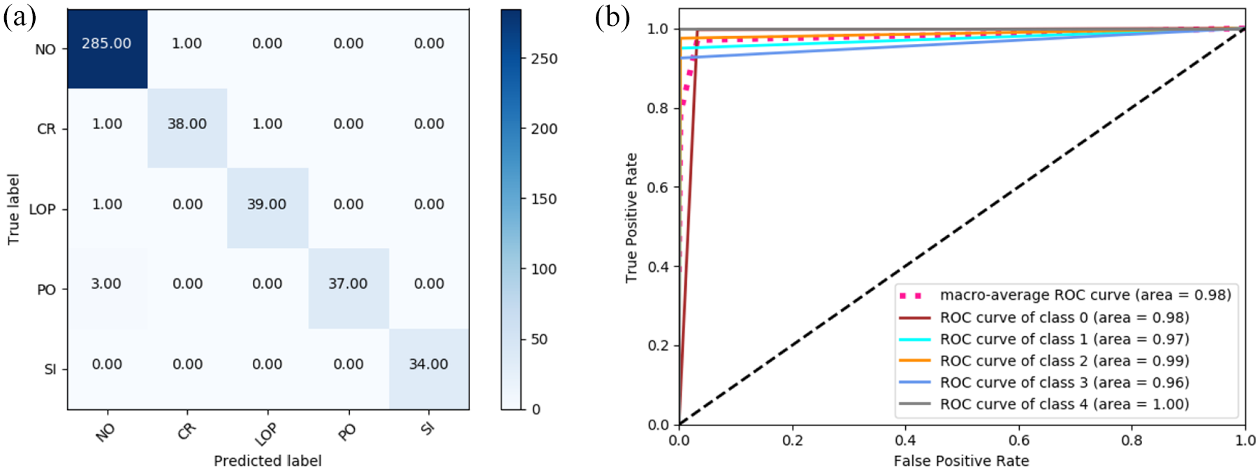
The confusion matrix and the ROC curve of the final results: (a) the confusion matrix and (b) the ROC curve.

Therefore, in the future classification process, in order to ensure better classification results, it is necessary to make the training images meet the conditions that the area of defect occupy most of the whole images.

Case analysis

In order to verify the robustness and generalization of the method, our method was used to verify the steel strip data set of Northeastern University (NEU).²⁴ And the classification accuracy of the model finally reached 97.78% when the number of each type of data set is {CR: 300, IN: 30, PA: 30, PS: 30, RS: 30, SC: 30}, which was better than some other machine learning methods. At the same time, the data set of real X-ray images of welding seams obtained from the space plant was selected for verification. Through our method, the classification accuracy of the model finally reached 98.83%.

Verified on the NEU dataset

The public data set used to verify the performance of the proposed method was derived from the NEU Surface defect database and consisted of six surface defect types, including cracking (CR), inclusion (IN), patch (PA), pitted surface (PS), rolled-in scale (RS), and scratch (SC). Each defect included 300 images, for a total of 1800 images which are processed at a resolution of 200 × 200 pixels. As shown in Figure 8.

Figure 8.

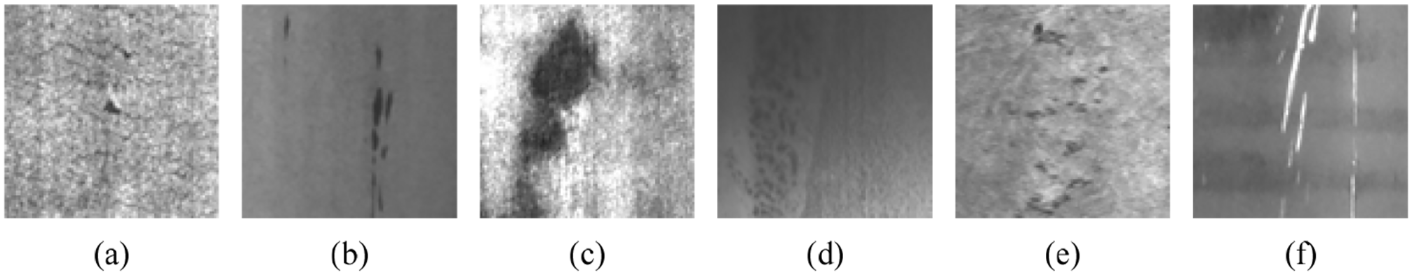
Six typical surface defect examples of NEU surface image database: (a) CR, (b) IN, (c) PA, (d) PS, (e) RS, and (f) SC.

Since all kinds of samples in the public data set of steel strip are balanced, we construct a new limited imbalanced dataset by selecting different number of pictures from the six categories of samples in turn. Three sets of imbalanced data sets were constructed, namely {300, 90, 90, 90, 90, 90}, {300, 60, 60, 60, 60, 60}, and {300, 30, 30, 30, 30, 30}.The total 450 pictures were divided into training set and test set according to the ratio of 8:2. We compared our proposed method with the traditional machine learning method and other deep transfer learning models. The final result shows that our method can achieve good recognition effect on the limited and imbalanced sample data set. The final experimental results are shown in Table 6.

Table 6.

Comparison results of different methods on NEU datasets. .

Datasets	Methods	Accuracy (%)	Precision (%)	Recall (%)	F1_score (%)
Whole of the images	KNN	75.00	—	—	—
	Random Forest	93.50	—	—	—
	SVM	87.11	—	—	—
{300, 90, 90, 90, 90, 90}	Fu et al.	98.00	97.62	97.22	97.42
	Ours	99.33	99.73	99.04	99.40
{300, 60, 60, 60, 60, 60}	Fu et al.	88.33	74.36	80.56	77.33
	Ours	99.17	99.73	98.61	99.17
{300, 30, 30, 30, 30, 30}	Fu et al.	78.89	37.40	49.72	42.69
	Ours	97.78	97.35	94.44	95.87

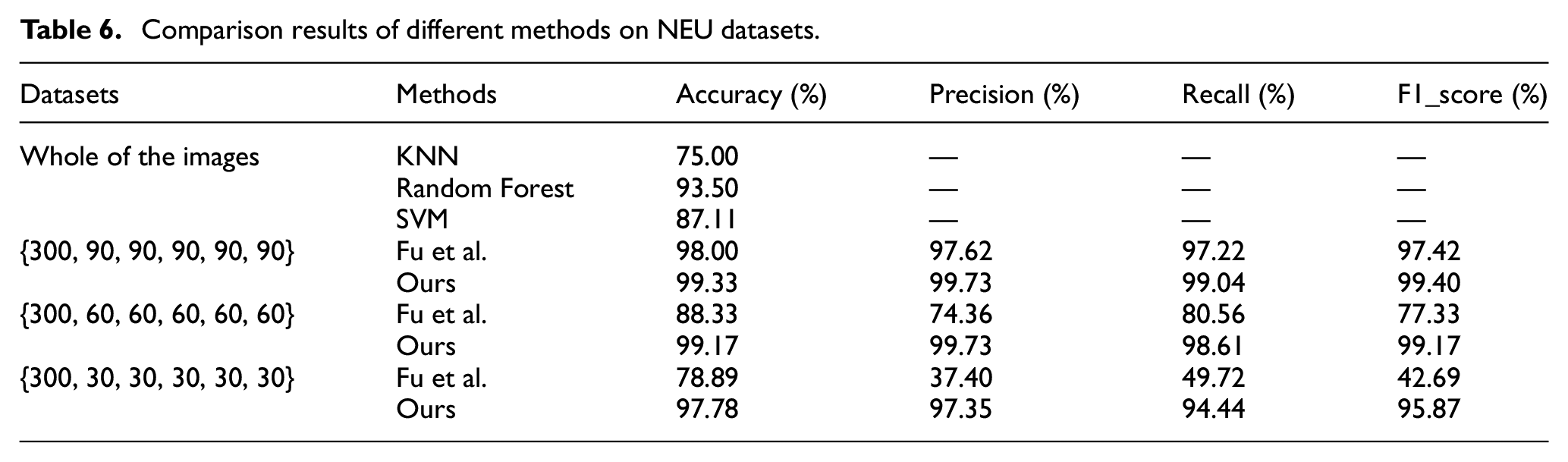
The experiment is compared with some traditional machine learning methods such as KNN, Random Forest, and SVM. And the experiment is also compared with a deep transfer learning model proposed by Fu et al.²⁵

The experimental results show that the traditional machine learning method can perform well when the sample size is sufficient and balanced. However, compared with the deep transfer learning method, feature extraction is required first and the process is more complex in traditional machine learning. Deep transfer model can automatically acquire image features and realize end-to-end image classification. And when the number of samples is small, deep transfer learning method can still achieve good classification accuracy. When the capacity of NEU dataset is {300, 90, 90, 90, 90, 90}, deep transfer learning method proposed by Fu et al. can perform well. But when the dataset become more imbalanced, the method will be influenced by those unevenly distributed samples. In the same circumstances of limited and imbalanced data, our model still has good robustness, which can reduce the influence of the majority of samples on classification results to a certain extent. Therefore, our method can effectively solve the problem of defect classification under limited and imbalanced samples.

Validation on real welding data

We obtained some real X-ray weld defect data from Plant A, and the defect types included internal and external defects of the weld. Four main defect types of images were obtained by clipping, namely tunnel holes (TH), flash burrs (FB), slag inclusion (SI), and lack of penetration (LOP). Similarly, the initial data set obtained by sliding window clipping is also imbalanced. Among them the defect categories and their corresponding images quantity is {TH: 77, FB: 172, SI: 425, LOP: 172}. As shown in Figure 9.

Figure 9.

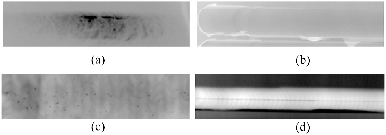
Four X-ray images of welds defect from Plant A: (a) TH, (b) FB, (c) SI, and (d) LOP.

The data set is divided into training dataset and validation dataset in a ratio of 8:2. The data set is trained with our method, and the final model performs well in the validation dataset. The data set is divided into training set and validation set in a ratio of 8:2. The data set is trained with our method, and the final model performs well in the validation set. The classification accuracy reached 98.83%. And other evaluation indicators also performed well: Precision reached 99.43%, Recall reached 97.72%, and F1_score reached 98.57%.

Through the above experiments, it can be found in Figure 10 that our model performs well not only on the public data set, but also on the real image data of weld seams. Especially when the image samples are insufficient and the sample categories are unbalanced, traditional machine learning methods generally perform not good enough, and it often takes a lot of time to expand the data set and train the new neural network from scratch. This indicates that our transfer learning method is more suitable for the classification of finite imbalanced samples than other methods, and the model can flexibly adjust the parameters of focal loss function according to the balance degree of samples. Compared to training model from the scratch, our final model size is 56.2 MB, less than half of the original model size (about 140 MB). This means that the DTN-VGG16 method has great potential in solving the problem of limited sample and imbalanced sample classification.

Figure 10.

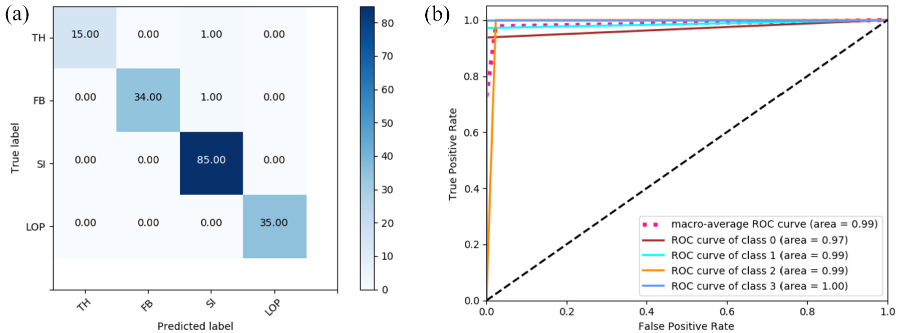
The confusion matrix and the ROC curve of the final results on real welding data: (a) the confusion matrix and (b) the ROC curve.

Conclusion

A deep transfer model based on VGG16 was proposed to realize defect detection on X-ray images of welds. The proposed method helps to solve the problem of the surface defect classification and to realize the automation of surface defects detection. In this method, some new layers were added on the basis of the pre-training model for fine-tuning, and the strategy of combining dynamic learning rate and focal loss function effectively solved the problem of small sample and imbalance dataset of defect classification, and the final model accuracy is stable at 98.41%. Moreover, compared with the transfer learning network based on other deep learning models, our model has better classification effect. And it is more accurate than traditional machine learning methods.

There are still some limitations in the research work of this paper: Clipping and marking images on the public data set requires the artificial prior knowledge, and the experimental results will also be affected by the marking quality of the data set. The amount of data is still not large enough. In order to further exert the advantages of the model, more images of defect types need to be collected. In the future, we will carry out further research on these limitations.

Footnotes

Acknowledgements

The authors express sincere appreciation to the anonymous referees for their helpful comments to improve the quality of the paper.

Declaration of conflicting interests

The author(s) declared no potential conflicts of interest with respect to the research, authorship, and/or publication of this article.

Funding

The author(s) received no financial support for the research, authorship, and/or publication of this article.

ORCID iD

Zaifang Zhang

References

Dong

Taylor

Cootes

. Automatic inspection of aerospace welds using X-ray images. In: 2018 24th international conference on pattern recognition (ICPR), Beijing, China, 20–24 August 2018, pp.2002–2007. New York: IEEE.

Hayes

. The ABC’s of nondestructive weld examination. Weld J 1997; 76: 46–51.

Chady

Sikora

Szwagiel

, et al. Multisource system for NDT of welded elements exploited in aircraft industry. COMPEL 2016; 35: 1478–1492.

Shen

Gao

. Automatic classification of weld defects in radiographic images. Insight Non-Destructive Test Condition Monitoring 2010; 52: 134–139.

Zapata

Vilar

Ruiz

. Performance evaluation of an automatic inspection system of weld defects in radiographic images based on neuro-classifiers. Expert Syst Appl 2011; 38: 8812–8824.

Yahaghi

Hosseini-Ashrafi

. Enhanced defect detection in radiography images of welded objects. Nondestructive Test Eval 2019; 34(1): 13–22.

Kumar

Anand

Srivastava

. Flaws classification using ANN for radiographic weld images. In: International conference on signal processing and integrated networks (SPIN), Noida, India, 20–21 February 2014.

Valavanis

Kosmopoulos

. Multiclass defect detection and classification in weld radiographic images using geometric and texture features. Expert Syst Appl 2010; 37: 7606–7614.

Guo

Zhou

. An intelligent monitoring system of grinding wheel wear based on two-stage feature selection and long short-term memory network. Proc IMechE, Part B: J Engineering Manufacture 2019; 233(13): 2436–2446.

10.

Wei

Yang

Liu

, et al. Railway track fastener defect detection based on image processing and deep learning techniques: a comparative study. Eng Appl Artif Intell 2019; 80: 66–81.

11.

Hou

Wei

Guo

, et al. Automatic detection of welding defects using Deep Neural Network. J Phys Conf Ser 2018; 933(1): 012006.

12.

Liu

Zhang

Gao

, et al. Weld defect images classification with VGG16-based neural network. In: Zhai

Zhou

Yang

(eds) International forum on digital TV and wireless multimedia communications. Singapore: Springer, 2017, pp.215–223.

13.

Hou

Wei

Jin

, et al. Deep features based on a DCNN model for classifying imbalanced weld flaw types. Measurement 2019; 131: 482–489.

14.

Cheplygina

de Bruijne

Pluim

JPW

. Not-so-supervised: a survey of semi-supervised, multi-instance, and transfer learning in medical image analysis. Med Image Anal 2019; 54: 280–296.

15.

Moore

Stammers

Dominguez-Caballero

. The application of machine learning to sensor signals for machine tool and process health assessment. Proc IMechE, Part B: J Engineering Manufacture 2021; 235: 1543–1557.

16.

Gong

Shao

Luo

, et al. A deep transfer learning model for inclusion defect detection of aeronautics composite materials. Compos Struct 2020; 252: 112681.

17.

Zheng

Zhao

Wang

, et al. Good practice in CNN feature transfer. arXiv preprint arXiv:1604.00133, 2016.

18.

Gopalakrishnan

Khaitan

Choudhary

, et al. Deep convolutional neural networks with transfer learning for computer vision-based data-driven pavement distress detection. Constr Build Mater 2017; 157: 322–330.

19.

Pan

Pang

Wang

, et al. A new image recognition and classification method combining transfer learning algorithm and MobileNet model for welding defects. IEEE Access 2020; 8: 119951–119960.

20.

Mery

Riffo

Zscherpel

, et al. GDXray: the database of X-ray images for nondestructive testing. J Nondestruct Eval 2015; 34(4): 42.

21.

Prati

Batista

GEAPA

Silva

. Class imbalance revisited: a new experimental setup to assess the performance of treatment methods. Knowl Inf Syst 2015; 45: 247–270.

22.

Lin

Goyal

Girshick

, et al. Focal loss for dense object detection. In: Proceedings of the IEEE international conference on computer vision, Venice, Italy, 22–29 October 2017, pp.2980–2988. New York: IEEE.

23.

Jadon

. A survey of loss functions for semantic segmentation. arXiv preprint arXiv:2006.14822, 2020.

24.

Song

Yan

. A noise robust method based on completed local binary patterns for hot-rolled steel strip surface defects. Appl Surf Sci 2013; 285: 858–864.

25.

Zhu

. Recognition of surface defects on steel sheet using transfer learning. arXiv preprint arXiv:1909.03258, 2019.

Image recognition of limited and imbalanced samples based on transfer learning methods for defects in welds