
Abstract
SwarmItFIX (self-reconfigurable intelligent swarm fixtures) is a multi-agent setup mainly used as a robotic fixture for large Sheet metal machining operations. A Constraint Satisfaction Problem (CSP) based planning model is utilized currently for computing the locomotion sequence of multiple agents of the SwarmItFIX. But the SwarmItFIX faces several challenges with the current planner as it fails on several occasions. Moreover, the current planner computes only the goal positions of the base agent, not the path. To overcome these issues, a novel hierarchical planner is proposed, which employs Monte Carlo and SARSA TD based model-free Reinforcement Learning (RL) algorithms for the computation of locomotion sequences of head and base agents, respectively. These methods hold two distinct features when compared with the existing methods (i) the transition model is not required for obtaining the locomotion sequence of the computational agent, and (ii) the state-space of the computational agent become scalable. The obtained results show that the proposed planner is capable of delivering optimal makespan for effective fixturing during the sheet metal milling process.
Keywords
Introduction
Currently, manufacturing industries are equipped with advanced technologies of higher flexibility potential due to the emergence of mass customization. 1 Especially sheet metal machining processes are becoming effortless due to technological advancements such as advanced CNC machining centers, tube laser cutting. However, positioning and orienting large sheets of metals using a conventional fixture setup is cumbersome. Improper fixturing may cause sheet metal deformation, which results in serious dimensional inaccuracies during machining. 2 Camelio et al. 3 have presented an optimization algorithm that proved to be reducing the dimensional inaccuracies by locating proper fixture positions for sheet metal assembly operations. Automotive industries update their product design once in every model year, which mandates the industries every time to update their fixture setup as well. 4 This fixture upgrade process is not only expensive but also increases the lead-time of the manufacturing process. Thus, to avoid such problems, industrial robot manipulators equipped with proper end effectors can be designed as reconfigurable fixturing systems. 5 Such reconfigurable robotic fixturing systems are technically termed as Robot Fixtureless Assembly (RFA). This RFA is capable of grasping, immobilizing, positioning, and orienting varieties of parts just by changing software commands. 6 Also, RFA reduces the workpiece reconfiguration time, which ultimately leads to a reduction in lead-time of the manufacturing process. The initial installation cost of RFA is slightly high when compared with conventional fixture setup. But finally, this RFA reduces around 20% of the total fixturing cost, 2 improves autonomy, 7 improves reconfigurability, 8 and ultimately increases the throughput.9,10 The workspace of the robot arm can be increased further by mounting it on the mobile platform. This facilitates the robotic machining of large-scale workpieces with higher positional accuracy.11,12
SwarmItFIX (Figure 1) is one such patented mobile RFA setup that supports sheet metals at the bottom when machining happens on top of the metal sheet.13,14 It follows the five-step sequence to traverse between any two support locations. These steps ensure coordination among head, PKM and mobile base agents of the SwarmItFIX, and each step corresponds to the sequence of locomotion of one agent. The novel Swing and Dock (SaD) locomotion strategy of the mobile base has already been explained in the previous works.15–17 Head is a vacuum type of end effector used to support the sheet metal on its bottom surface. For the head to reach the specific coordinate within the workspace, the cooperation of all the three agents become essential. SwarmItFIX is a redundant manipulator with a 4R serial arm (R – Rotational) mounted on a Parallel Kinematic Machine (PKM) having three limbs. Two limbs are with the kinematic architecture of RRPR, and the other is with SPR (P – Prismatic, S – Spherical) configuration. The design is in such a way that the PKM is to accomplish the positioning task, whereas the serial arm is to orient the end-effector head. The PKM with the serial arm provides six Degrees of Freedom (DOF) pose together. The SwarmItFIX head has a dedicated motor and hence, an independent DOF to accommodate the orientation of the head along with the sheet metal. This enables de-coupling in inverse kinematics, where only the six DOF pose of the end-effector vacuum head is mainly required and hence, orientation can be achieved independently. The detailed kinematic analysis of the PKM has already been done. For the PKM, only the six-dof pose/Euler angles of the end-effector (head) with respect to the base are required to achieve a feasible path based on the methodology proposed. Once target orientation of the head and position of the base are obtained, the motion trajectory of the PKM can be generated between the two positions based on the inverse kinematics model. 18 The entire manipulator is mounted on a mobile base with a harmonic drive to provide an additional DOF of rotation. Hence, the kinematic structure of the SwarmItFIX robot is specially designed to be redundant to provide at least one solution to the motion planning problem. Various heuristic approaches are proved to be promising in the robot path planning and domain. 19 But the problem is that these methods do the computation again when the same goal positions are repeated, that is, no policies are stored.
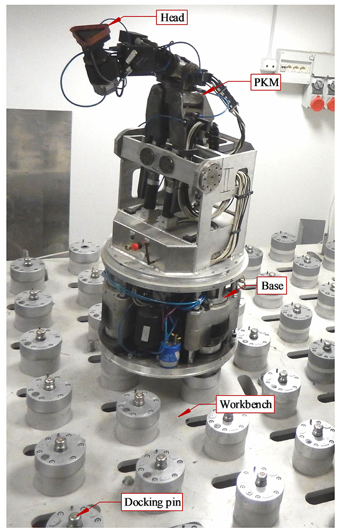
SwarmItFIX setup at the University of Genoa, Italy.
Reinforcement Learning is a viable alternative for the conventional techniques in the path planning domain. RL overcomes shortcomings such as replanning and detour. This technique uses the rewards observed by the computational agent while taking appropriate action in each state to learn the optimal (or nearly optimal) policy. Then, using this optimal policy, the sequence of operations performed by the physical agent can be computed. 20 Initially, the computational agents would not have any knowledge about the optimal policy, but they learn the same by interacting with the computational environment.21,22 The skills acquired by the computational agents can be evaluated by using the intrinsic motivations in the RL framework. 23 This optimal policy learned by the computational agent can be transferred to the robots for its optimal locomotion.24,25 The authors have utilized two different algorithms, viz, extended single-agent Q-learning algorithm and Team Q-learning algorithm, for a fully cooperative multi-robot box pushing task. 26 Though single-agent Q-learning is developed for static environments, it still copes with the dynamic environment (environment with more than one agent) and offers positive and better results when compared with the Team Q-learning algorithm. The same authors have also presented Sequential Q-learning with Kalman Filtering (SQKF) algorithm, which is a modified version of the distributed Q-learning algorithm for the same task. 27 SARSA obtains better state estimates for mobile robot delivery tasks when compared with other RL approaches as confirmed by Ramachandran and Gupta. 28
Numerous ways have been explored by the researchers for solving inverse kinematics of the robot mechanisms. The inverse kinematic analysis of any parallel manipulators which resembles the Stewart platform can be effectively performed using homogenous transformations. Also, the solvers which utilize multidimensional geometric information of the mechanism, efficiently solve inverse kinematics problems. The geometric constraints of the mechanisms can be satisfied by devising a fixed sequence of actions which ultimately reduces the degree of freedom of a mechanism.29,30
The objectives of the present work are;
to develop a hierarchical RL based path planner for the path planning of head and base agents of SwarmItFIX,
to develop a methodology for the identification of goal positions of the SwarmItFIX-base in line with all support locations,
to formulate the path planning problem of SwarmItFIX base agent as MDP for a fixed-size environment that is scalable for the larger size environments,
to propose a unique reward function that enables the computational agent to explore the environment,
to identify and utilize a suitable model-free reinforcement learning technique for solving the formulated MDP, and
to test the proposed planner with various tool trajectories.
The rest of this paper is organized as follows. The research gap and problem definition are detailed in section 2. The five-step locomotion strategy is explained in section 3. Details of MDP modeling and the proposed RL based offline architecture is presented in section 4. The results are discussed in section 5. Conclusion statements and details of future works are described in section 6. Followed by references.
Research gap and problem definition
Based on the detailed literature survey, it has been confirmed that,
• To consecutively provide support throughout the machining process, the agents of the robot must coordinate in a sequential manner. The existing hierarchical CSP approach which performs this coordination has the following issues that need to be addressed.31,32
The hierarchical CSP approach only computes the goal positions of the SwarmItFIX base and not the sequence of locomotion. This is with the condition that the two consecutive goal positions should have a common docking pin; otherwise, the planner would fail.
When the base CSP fails to identify such goal positions, it tracks back and forces to replan to find a new head position. This replanning procedure causes unnecessary detours.
• To overcome these issues, a planner with the liberty of choosing the goal positions more flexibly and capable of computing the locomotion sequence of SwarmItFIX base need to be developed.
• The action sequence of the SwarmItFIX base agent has to be computed with reduced makespan and minimum learning time and without any backtracking or replanning. The term makespan here denotes the number of steps required to be performed by the SwarmItFIX for accomplishing the given task (for reaching the goal position). The minimal makespan would facilitate the machining with a higher feed rate, which ultimately increases the throughput of the system.
The five-step locomotion of SwarmItFIX
In order to traverse between two support locations, all agents of the SwarmItFIX robot have to coordinate by performing the locomotion of each agent in a sequential manner. The mobile base acts as a primary locomotion source which traverses the robot to various locations within the workbench. When the robot reaches the defined location, the mobile base locks its position to support the workpiece. Now, the PKM positions the equilateral triangle shaped head in the defined support location along with the required orientation. The PKM is linked with a three DOF 3R spherical wrist which gives the additional DOF needed for the orientation of the head. Let (hj, bj) and (hj+1, bj+1) be the position of the head (h) and base agent (b) at support locations j and j + 1, respectively (Figures 2 and 4). The transition (positioning alone) between hj and hj+1 is due to the movement of PKM and base. The associated orientation is taken care of by the independent rotational motion of the head alone. Starting from the jth supporting position (hj, bj), the SwarmItFIX robot performs the following five-step transitions and reaches the next supporting position (hj+1, bj+1).
Transition 1: Retraction of the head away from current support location of the work-piece (hj).
Transition 2: Movement of the head agent to parking position to avoid collision with other agents.
Transition 3: Locomotion of base (bj→ bj+1) along with the simultaneous counter-rotation of the PKM (Figure 2). As the PKM is already parked safely, the collision-free locomotion of the whole manipulator at this stage is completely ensured.
Transition 4: Movement of head to a nearby position which is a normal approach away from next support location hj+1.
Transition 5: Movement of the head to the next support location of the workpiece hj+1.
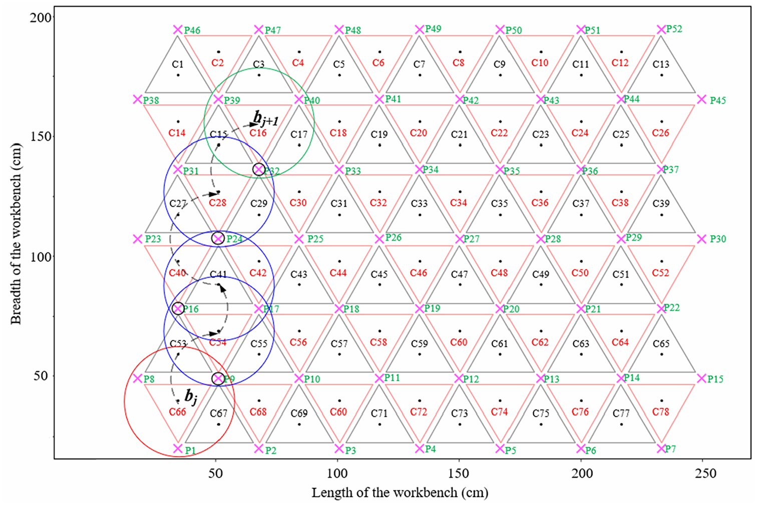
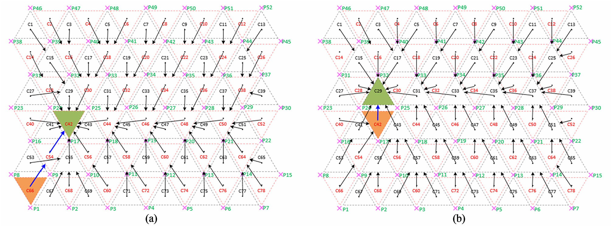
SaD locomotion of the base agent (The positions sequence: C66→C54→C41→C28→C16; sequence of docked pins during locomotion: P9→P17→P24→P32).
Reinforcement learning based path planner module
This section presents the proposed planner (Figure 3), which works based on the coordination of various agents of the SwarmItFIX robot.
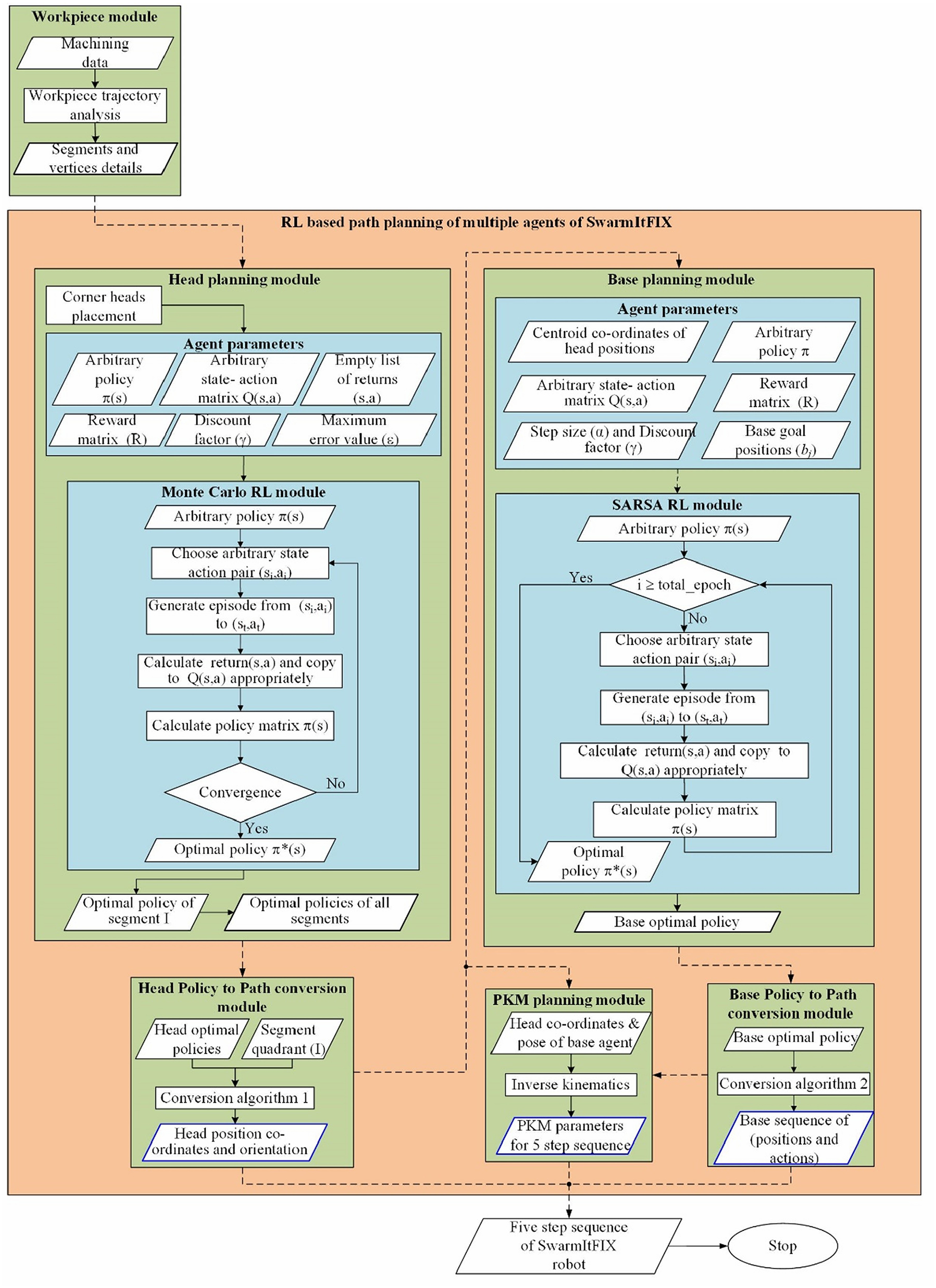
RL based offline path planner.
The proposed path planner module
The proposed path planner module developed based on Reinforcement Learning for the coordination of multiple agents of the SwarmItFIX robot is shown in Figure 3. This path planner basically comprises two major modules; the head planning module along with the Monte Carlo RL module, which was proposed earlier and the newly proposed base planning module along with the SARSA RL module.
Workpiece module
The workpiece module gets executed once for each tool trajectory. It analyzes the tool trajectory obtained from CAM software, and splits the complete trajectory into various linear segments and then calculate the angular information of all segments and these are called vertex angles. This module also calculates the number of vertices present along the trajectory and their type and number of segments.
Multi-agent RL module
Based on the data received from the previous module, this multi-agent module computes the position and orientation of vertex heads initially and then proceeds to the head planning submodule. This submodule computes the position and orientation of intermediate head positions as given in Figure 3.
Base planning module
The first step in this module is the identification of goal positions (bj) for all head support locations (hj) in the workbench (Figure 4). Hence, the coordinates of hj are utilized for the computation of goal positions. In this regard, initially, a polygon is created with projections of centroids of head support locations 1 (h1) and 2 (h2) on the workbench as the two inner corners e1 and e2, respectively. The two outer corners of the polygon e3 and e4 are calculated using equations (1) and (2). Finally, the base positions in the workbench, which satisfies the constraints of equations (3) and (4), are considered as the goal positions (bj) of the base agent.
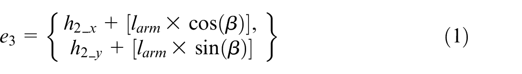
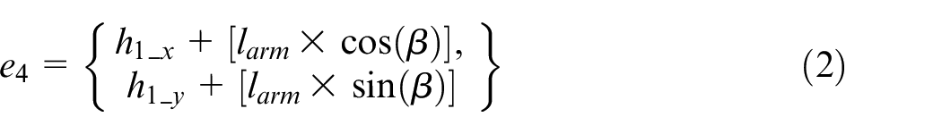


where, Ccd is the coordinate of the centroid of base position. T1, T2, T3, and T4 are the areas of triangles formed by the vertices e1, e2, e3, e4, and Ccd. sd is the safest distance considered between trajectory and base, and it will act as an important parameter to avoid collision between two base agents. larm is the length of the serial arm. β is the angle of the line segment connecting two corner positions of a polygon.
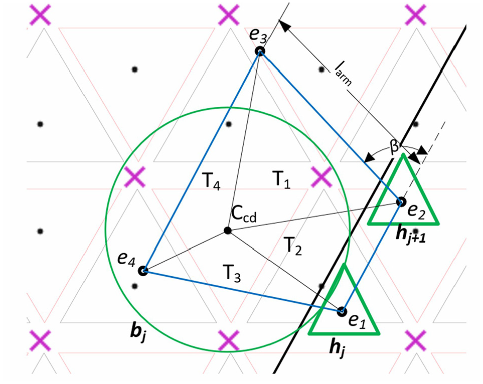
Identification of base goal positions.
Now for making the base agent traverse between the current position (bcurr) and the goal position (bj), a policy that is capable of suggesting an optimal sequence of actions with the objective of minimizing the makespan is required. Basically, the base agent traverses on the modular workbench, where its dimensions can be scaled based on the size of the workpiece. Hence, this path planning problem is modeled as Markov Decision Process (MDP), and the SARSA model-free RL algorithm is utilized to solve it.
SARSA Temporal Differencing (TD) algorithm is defined by the quintuple <si,ai,ri,si+1,ai+1> that perform transitions between ith state-action pair and i + 1th state-action pair and learns the state-action values Q(s,a). Whereas, in the other model-free RL algorithms, such as MC control, the transitions are performed between two different states, si and si+1. Various agent parameters used in the SARSA base planning module are:
State space (s∈S)− As shown in Figure 2, the workbench consists of 52 docking pins (Np) and each of which combines with neighboring docking pins and form triangular configurations of 129 edges (Ne) in total. Using Euler’s relation equation (5), the number of possibilities of obtaining the base position (Nb) is found to be 78. Thus, the state space S contains 78 states in a pattern of a triangular grid which comprises 6 rows and 13 columns.

Action space (a ∈ A)– Each state shares the docking pins with 13 neighboring states. Hence, from any particular state, an agent could perform 13 different actions (B0–B12) to reach the neighboring states. Out of these 13 actions, B11 and B12 are not considered in the action space due to the following reasons.
When these two actions are performed on an odd-numbered state, the computational agent reaches bcurr+11 and bcurr+15. Whereas, if it is performed on an even-numbered state, it reaches two different states, bcurr − 11 and bcurr − 15.
These states can also be reached by performing the other actions twice consecutively.
Hence, for the locomotion of the base agent, 11 different actions (B0–B10) can be assigned. Figure 5 describes the details of action space. The details of corresponding locomotion for all the actions are presented in Table 1.
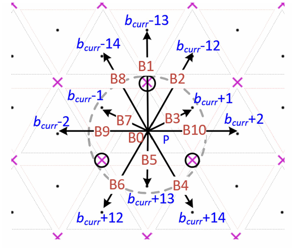
Action space.
Actions and locomotion mapping.
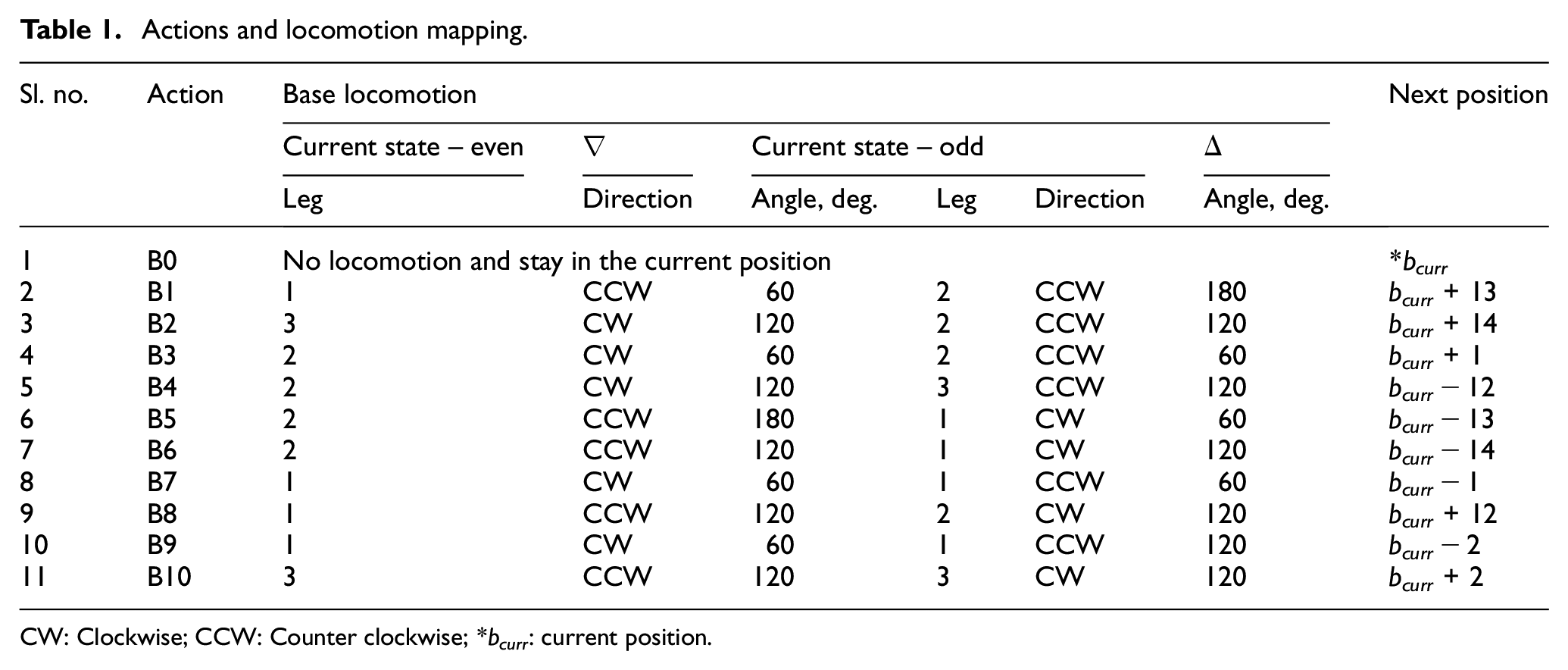
CW: Clockwise; CCW: Counter clockwise; *bcurr: current position.
Reward matrix R(s,a) – The reward matrix is constant throughout the process, and it is calculated as below.
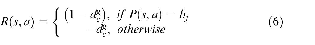

where,
State-action matrix Q(s,a) – The size of the state action matrix is 11 × 78 (actions × states).
Step size (α) – It is a factor (
Discount factor (γ) – It plays a major role in choosing between the current rewards and future rewards. It also varies similar to α. When γ gets close to 0, the future rewards become negligible. When γ gets close to 1, more importance will be assigned to future rewards.
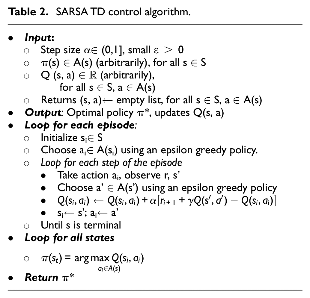
The operation of the SARSA algorithm (Table 2) begins with choosing the arbitrary state-action pair (si,ai), and the state si will be the initial state of the episode. The corresponding Q-value will be calculated using equation (10) and will be updated in the state-action matrix Q(s,a) against the corresponding initial state-action pair (si,ai). Finally, the optimal policy (π*) obtained will provide an efficient base action sequence for all the support locations of the tool trajectory.
SARSA TD control algorithm.
The expected return (τ) of the state can be calculated using equation (8).
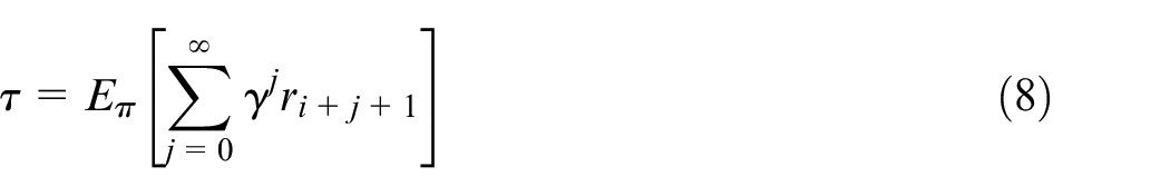
which can be further simplified as under
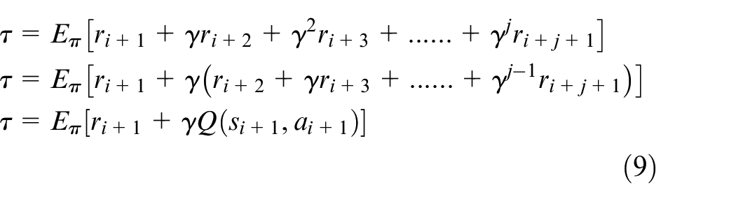
The update rule for the SARSA-TD control algorithm is given in equation (10).
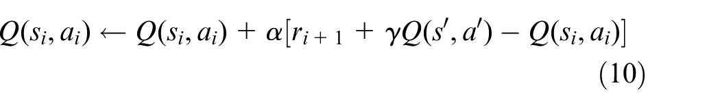
ri +1 defines the reward obtained at the state si+1, j is the weightage parameter of the discount factor for the future rewards. Based on the calculated state-action matrix Q(s,a), the policy matrix will also get updated.
Base policy to path conversion (BPP) module
Given the respective start positions, this BPP module gathers about π* from the base planning module and converts them into a sequence of states and actions. Initially, for the first sequence, the home position will act as the start position. Now, this module refers to the first optimal policy and computes the sequence of actions. The base agent needs to perform this sequence in order to reach the goal position (b1). Similarly, in the second sequence, positions b1 and b2 are the start and goal positions. This process gets iterated until the sequence for all the goal positions (bj) are obtained.
PKM planning module
As mentioned earlier, the PKM module is equipped with a fixed sequence of actions. For all the goal states of the head-base pair, the PKM traverses in a fixed sequence and facilitates the head agent to reach the goal state. Given the target position of the head, by using the existing inverse kinematic model, the state variables of the PKM can be calculated.
Results and discussion
Simulation of multi-agent path planning of the robot is carried out using a novel RL based planner proposed in this work. The configuration of the system used for simulation includes Intel Xeon CPUE3-1225v6 Processor 3.30 GHz, Windows 10, 64-bit OS with 16.0 GB RAM. Mathematical models are implemented using Python 3.7 idle interface. The results obtained are grouped under three categories and presented as follows.
Estimation of RL parameters
The path planning problem of the base agent of the SwarmItFIX robot is modeled as Markov Decision Process (MDP), and model-free Reinforcement Learning (RL) algorithm viz., SARSA TD control is deployed to solve the MDP. Initially, the optimum values of various parameters of the SARSA algorithm are estimated as detailed below.
Five different test cases, C1 as goal position and C20, C6, C35, C52, and C78 are the various start positions are considered. Hence, the distance between the start position and the goal position in all the cases are different from each other.
Initially, a simulation experiment is executed for finding the optimal discount factor (γ) within the range 0.8 ≤ γ < 1 based on literature. The corresponding result obtained is shown in Figure 6(a). When γ < 0.96, the computational agent could not reach the goal position even after 1000 steps for cases with higher distances between start and goal positions (C52 and C78). The process also gets terminated for such cases. For the other three cases (C20, C6, and C35 as start positions), the computational agent reaches the goal position.
By increasing the γ value further, the computational agent finds the goal position for all the test cases. But when γ is close to 1, the goal position is attained in all the cases with the least execution time (37.15 s).
Similarly, experiments are carried out for finding optimal step size (α), greedy value (ε), and the number of iterations (n) and the associated results are presented in Figure 6(b)–(d), respectively. The optimal values found are γ = 0.999, α = 0.1, ε = 0.1, and n = 35,000.
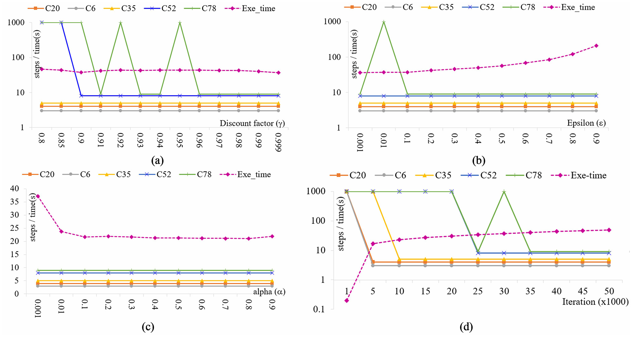
RL parameters estimation: (a) discount factor, (b) greedy value, (c) step size, and (d) number of iterations.
Convergence of optimal policies
The results obtained while executing the SARSA algorithm for base agent planning of the SwarmItFIX robot are discussed now. The goal positions of the base agent are calculated by applying equations (1) and (2), and the total number of goal positions (bi) is calculated as sixteen for the tool trajectory.
The base agent, from its start position, performs a sequence of actions and reaches each goal position. As the trajectory contains 16 goal positions, the base agent needs to perform 16 sequences to cover the complete trajectory. Thus, 16 different optimal policies are required for the base agent. For the first sequence, the home position C66 become the start position, and C42 become the corresponding goal position (b1). Similarly, C42 and C29 are the start and goal (b2) positions, respectively, for the second sequence.
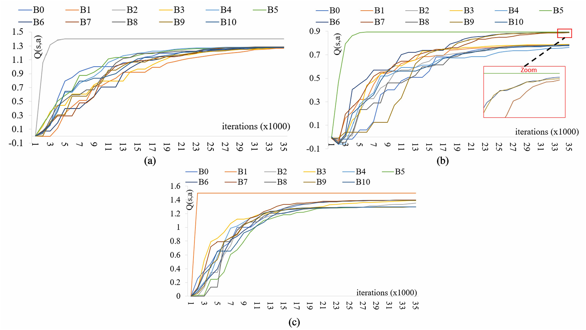
The three plots in Figure 7 show the Q-values of all 11 actions of 5 different states. Figure 7(a) and (b) corresponds to the first sequence (
Further, it can be observed in the first sequence at state C66 (Figure 7(a)) that, when the iteration progresses, the Q-value of action B2 increases at a faster rate when compared with the Q-values of the rest of the actions. This clearly shows that in the first sequence at C66, B2 is the optimal action that is recommended for the base agent. Similarly, optimal action for C13 (first sequence) and optimal action for C42 (second sequence) can be observed from Figure 7(b) and (c), respectively.
From Figure 7(c), it can be observed that action B1 is immediately converged as an optimal action when compared with the actions B2 and B5, as shown in Figure 7(a) and (b), respectively. This is due to the fact that, in the second sequence, the state C29 is the start position which is a neighboring state of goal position C42. Hence, the distance
The convergence of the optimal policy for the first two sequences is shown in Figure 8(a) and (b) by plotting the step length of the episodes of all the iterations. For both sequences, the path planner has been executed with two different sets of RL parameters. Set 1 comprises of identified optimal values γ = 0.999, α = 0.1, ε = 0.1, whereas, the corresponding values for set 2 are γ = 0.85, α = 0.001, ε = 0.01. In the first iteration of both sets, the computational agent starts from a random state, follows a non-optimal policy, and takes more than 500 steps to reach the goal state. But, when the iteration progress, the policy converges gradually and becomes optimal. Finally, the agent reaches the goal position in fewer steps. It can also be observed from both the sequences that set 1 with the optimal parameters converge much faster than that of set 2.
Q-values versus actions: (a) optimal policy 1 state C66, (b) optimal policy 1 state C13, and (c) optimal policy 2 state C42.
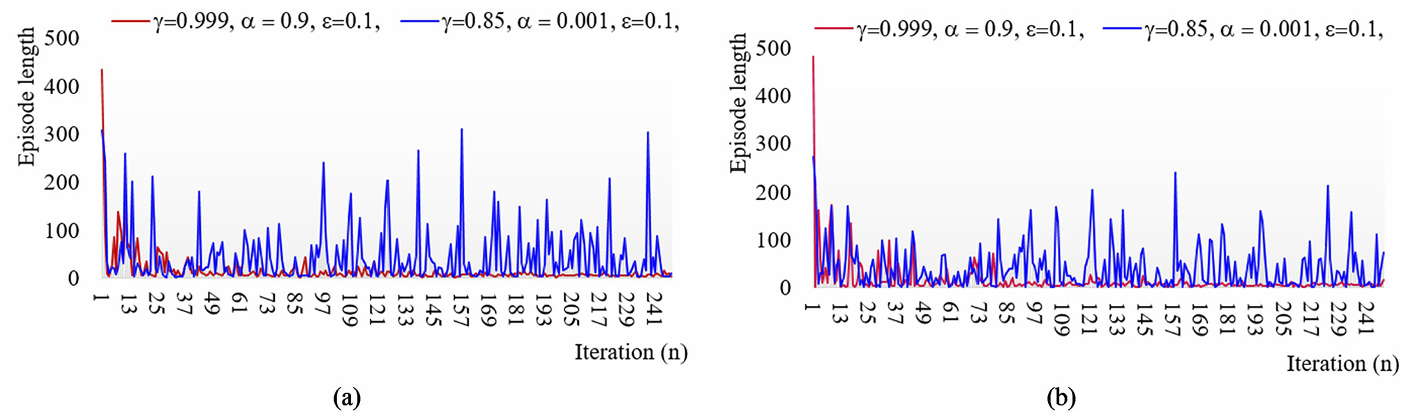
Learning curve: (a) first sequence and (b) second sequence.
Execution on various tool trajectories
The optimal policies for both first and second sequences are shown in Figure 9(a) and (b), respectively.
The arrows shown at the states indicate the action of the corresponding state recommended by the optimal policy (π*). States C42 and C29 become the goal positions of the first sequence and second sequence, respectively.
When starting from any state with the help of these optimal policies, the sequences for reaching the corresponding goal positions can be obtained in an efficient manner. Finally, when all sequences are combined for completing the trajectory, the agent performs 23 locomotion steps starting from the home position to the last goal position while passing through all intermediate goal positions.
The details of actions performed and rewards earned by the agent at each locomotion are depicted in Figure 10. The planning model has also been tested with various trajectories, and the results are shown in Figure 11. It confirms the placement of both head and base agents based on the outcome of the planner. In the placement of the base agent, the continuous circles (green) represent the goal positions of the base agent, whereas the discrete circles (blue) become the intermediate positions. The lines (red) that connect the base goal positions and head positions denote the active states of PKM and head agents.
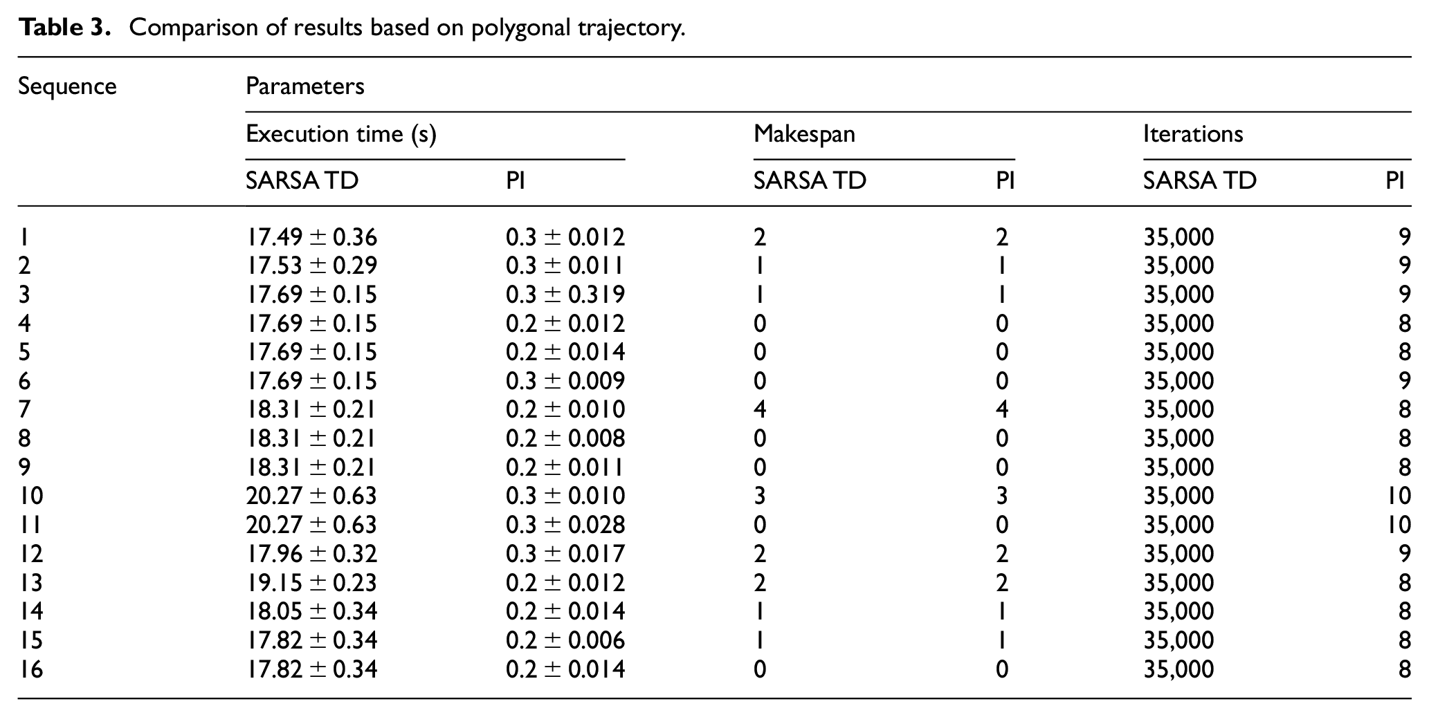
Table 3 compares the SARSA algorithm with the baseline Policy Iteration (dynamic programming) algorithm in terms of computation time, makespan, and the number of iterations iteration for all the 16 sequences of the polygonal trajectory shown in Figure 11(c). It can be clearly observed that the SARSA algorithm produces optimal results in terms of makespan.
Optimal policy: (a)
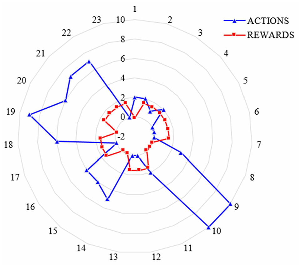
Actions and rewards obtained by base.
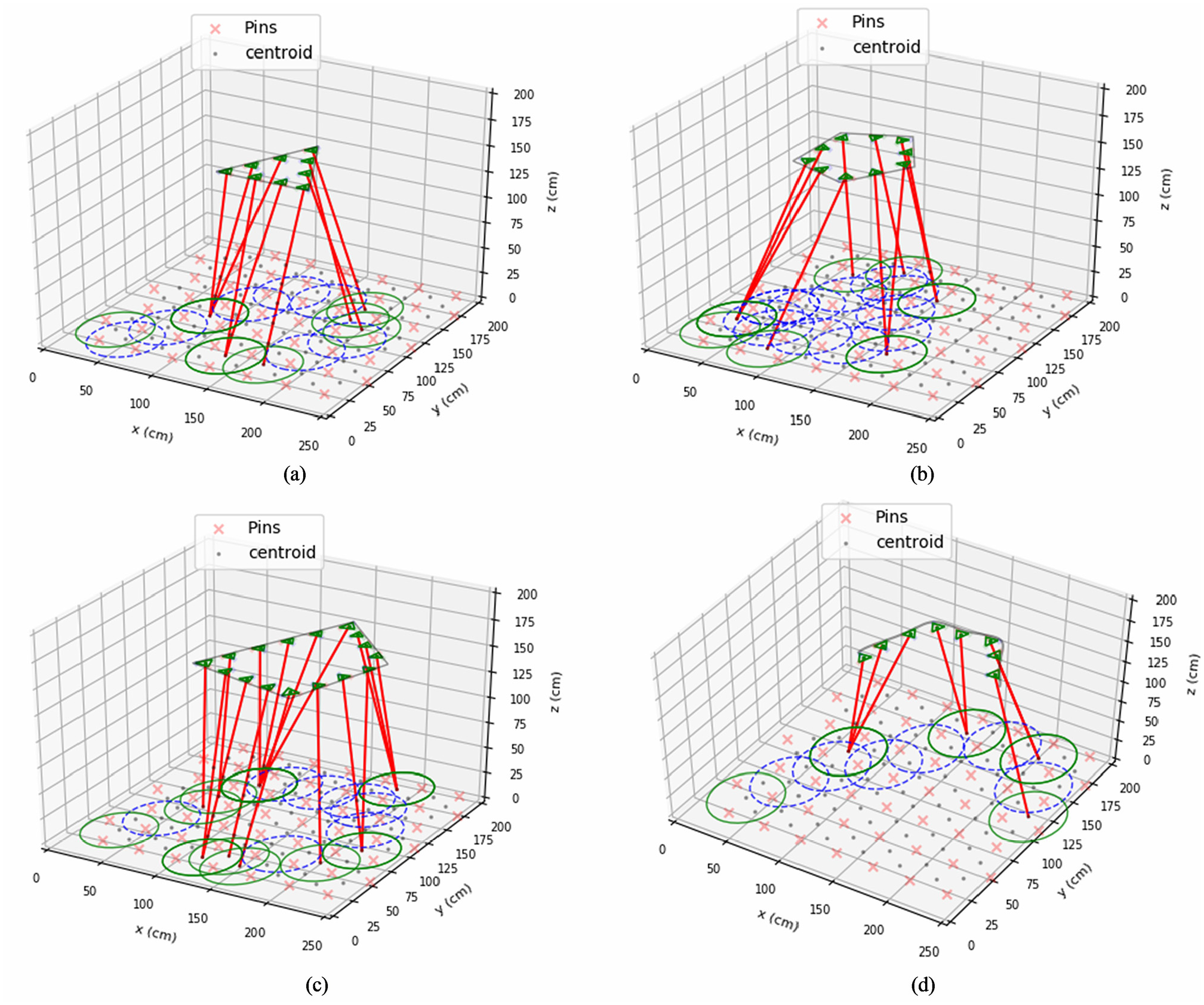
Head and base placement on other tool trajectories: (a) triangular trajectory, (b) pentagonal trajectory, (c) polygonal trajectory, and (d) open curved trajectory.
Comparison of results based on polygonal trajectory.
Conclusion and future work
In this work, a model-free RL based path planner is developed and presented for the coordination of multiple agents of a SwarmItFIX robotic fixture. Based on the results obtained, the following conclusions are drawn.
The proposed path planner is found to be an efficient in terms of achieving the coordination among multiple agents of a single SwarmItFIX robot. The disadvantage of having a replanning procedure present in the previous CSP approach has been avoided by the proposed SARSA TD based planner. Hence, replanning and detour are eliminated.
Initially, the Monte Carlo based RL algorithm was deployed for the computation of base agent optimal policy for five test cases, as shown in Figure 6. Though there is no difference in the optimal policies produced by both the algorithms, the SARSA algorithm computes the optimal policy nine times faster than the MC algorithm (360 s vs 40 s). Hence, the major part of this research work is carried out based on the SARSA algorithm.
The optimal value of the parameters used to conduct the experiment are found to be γ(discount factor) = 0.999, α(step-size) = 0.1, ε(greedy value) = 0.1, and number of iterations = 35,000. With these optimal values, the SARSA TD algorithm has been executed further for obtaining the desired action sequence for various trajectories, as shown in Figure 11. Finally, the results obtained are compared with the results of the baseline model-based Policy Iteration (PI) algorithm, as presented in Table 3.
The proposed SARSA based model works well with all the test cases of simple machining trajectories, as shown in Figure 11. A compatibility check of the proposed planner for complex curved trajectories is proposed for future research. The possibilities of utilization of the SwarmItFIX robot as a robotic fixture for other machining operations will also be investigated.
Multi-robot planning is more complex when compared with the planning of multiple agents of one SwarmItFIX robot. This is because the environment becomes dynamic, and the locomotion of one robot becomes the moving obstacle for the other. Thus, in future, the same model-free RL based planning scheme will be extended further to solve this dynamic multi-robot path planning problem.
Footnotes
Appendix
Acknowledgements
The support being received from Prof. Matteo Zoppi, Prof. Rezia Molfino, and Dr. Keerthi Sagar of PMAR Research Group @ The University of Genoa is highly acknowledged.
Declaration of conflicting interests
The author(s) declared no potential conflicts of interest with respect to the research, authorship, and/or publication of this article.
Funding
The author(s) disclosed receipt of the following financial support for the research, authorship, and/or publication of this article: This work is an outcome of the sponsored project (Project No: MEC/DIMEUG-ITALY/2015-16/MSK/008/02) with a financial grant from the University of Genoa, Italy.