
Abstract
The determination of AGV vehicle requirements in a manufacturing system has a great impact on the system performance. This paper first defines the AGV vehicle requirement determination as a general optimization problem, and secondly develops a new AGV vehicle requirement determination method capable of effective solving the problem. This method features with the combination of discrete event simulation (DES), sensitivity analysis, fractional factorial design (FFD) and response surface methodology (RSM). Tests and comparisons with other simulation based methods have shown that the proposed method combining the simulation method with analytical method, can make full use of their respective advantages and overcome the defects of existing methods. It is more practical.
Keywords
Introduction
Automated Guided Vehicle system (AGVS) is a driverless material handling system (MHS) used for horizontal movement of materials. AGVS has been frequently used in a manufacturing system in order to improve the system performance by rapidly responding to different changes in the demand, product mix and job priorities. The use of AGVS makes a manufacturing system more flexible, productive and cheaper per unit. 1 In order to make the entire system run efficiently, a certain number of AGVs needs to be properly parameterized and configured into the manufacturing system. This naturally brings up a problem of how to determine vehicle requirements at strategic level in the design of manufacturing system according to the survey of several review papers (Vis, 2 Ganesharajah et al., 3 Le-Anh and DeKoster 4 ). The AGV vehicle requirement is related to the determination of vehicle ontology parameters required by the manufacturing system, including AGV number, AGV type, AGV speed, AGV capacity, AGV acceleration, AGV loading time and unloading time, etc. These variables can synthetically determine the efficiency of logistics and thus affect the performance of manufacturing system such as the completion time, throughput, investment cost, equipment utilization etc.
In the related research field of determining vehicle requirements of AGVS, both analytical approaches and simulation are used to solve the problem. Mathematical programming, queueing theory, network models and regression analysis have been used to solve relatively small problems where a problem can be simplified and formulated as an analytical model. For example, Johnson and Brandeau 5 suggested formulating a vehicles requirement problem as a binary integer programming model and solving it with enumeration algorithms. Ji and Xia 6 proposed an approximately analytical method to analyze vehicle requirements in a general AGV system. Some researchers used analytical approaches to determine the number of AGV vehicles and the fleet sizes. Rajotia et al. 7 discussed a mixed integer programming model to determine optimal AGV fleet size in a flexible manufacturing system (FMS) for minimizing empty trips of vehicles. Arifin and Egbelu 8 used a regression technique to estimate the number of vehicles during the initial phase of a system design. Choobineh et al. 9 modeled the movement of AGVs as a multi-class closed queuing networks (CQN), and the AGV’s fleet size was estimated by a linear program. Chawla et al. 10 carried out an investigation for fleet size optimization of AGVs in different layouts of FMS by blending analytical method and gray wolf optimization algorithm. The above analysis methods are difficult to be universally applied without a unified form. Moreover, different models either under-estimate or over-estimate the actual number of vehicles required. 7 In contrast, the simulation approach has been successful in modelling such a complex dynamic system and has been proven to provide an accurate number of vehicles required. 8 A few authors addressed the problems of vehicle requirements of AGVS by means of simulation. Gobal and Kasilingam 11 presented a SIMAN based simulation model to determine the number of AGVs needed to meet the material handling requirements. Hamdy 12 developed a simulation model to determine the optimized number of AGVs while simultaneously considering the battery management of the AGVs. Um et al. 13 presented a hybrid method that combined simulation-based analytical and optimization techniques to satisfy three system objectives of minimizing congestion, maximizing vehicle utilization and maximizing the throughput. Lin et al. 14 and Huang et al. 15 proposed simulation optimization approaches to determine the optimal number of vehicles in wafer fab. Tao et al. 16 proposed a two-step combined analytical and simulation method for estimation of AGVs requirement. Pjevcevic et al. 17 applied data envelopment analysis and discrete-event simulation for determining an efficient AGV fleet size. Valmiki et al. 18 summarized significant papers reported in the field of AGV fleet size estimation, and concluded that simulation methods give better results but in complex situations, simulation methods are cumbersome. In addition, there are other proposed methods for this research problem such as iterative learning 19 or repetitive learning. 20 The simulation approach seems to be a relatively good method, however, it lacks a clear mathematical analytical form, large number of simulation experiments need to be performed, which makes it costly, tedious and time-consuming.
From the above brief literature review, it is worth noting that most related works take the AGV vehicle requirement problem as the AGV fleet sizing problem or minimum AGV number problem. In fact, the vehicle requirement of AGVS also includes other AGV parameters such as AGV speed, loading time, unloading time etc. These parameters are just as important as vehicle number and should be taken into account simultaneously.
To overcome the limitations of existing approaches, a general and effective method is needed by combining simulation and analytical models for the design and analysis of vehicle requirements of AGVS. Therefore, along this vein, this paper proposes a new general method by combining the existing DES, FFD, and RSM to be capable of obtaining the combinatorial optimal values of vehicle ontology parameters. It has the advantages embedded with both analytical and simulation methods, providing a systematic solution with universal adaptability. Compared with the existing research, the main contributions of this study are as follows:
(1) A new method to solve a general AGV vehicle requirement problem, which enables not only the optimal determination of the number of vehicles and fleet sizes, but also others parameters described in the AGV ontology.
(2) The proposed method effectively combines the existing DES, FFD, and RSM to provide a robust framework for design and analysis of vehicle requirements of AGVS in a flexible manufacturing system. It is more practical when compared with Genetic Algorithm (GA)-based/Particle Swarm Optimization (PSO)-based simulation optimization, showing that it can reduce the number of experiments while obtaining the same optimal solution.
The remainder of the paper is organized as follows: The problem is defined in Section 2. Section 3 describes a systematic method combining DES, FFD, and RSM in optimization design of vehicle requirements of AGVS. In Section 4, a simulation model for the AGVS is proposed and the experimental validation is performed. The comparison between the proposed method and GA-based/PSO-based simulation optimization method is provided in Section 5. Finally, the conclusions are drawn in Section 6.
The problem formulation in vehicle requirement of AGVS from a systematic perspective
The general mathematical model for AGV vehicle requirement problem can be described as follows:
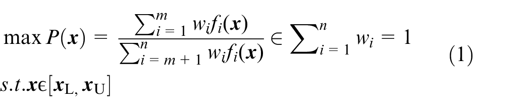
Where
The equation (1) may not have an analytic expression and can only be estimated by simulation with noise consequently. So quite a lot of simulation observations are needed to identify the optimal solution, which are computationally unaffordable in practice if there are many variables. It is necessary to develop a methodology to quickly determine the optimal solution with reasonable amounts of computations.
The optimization method for solving the problem of vehicle requirement of AGVS
In this paper, we present a systematic approach called RSM simulation metamodel (RSMSM) for design and analysis of vehicle requirements of AGVS in manufacturing systems. The flow chart of overall approach is illustrated in Figure 1.
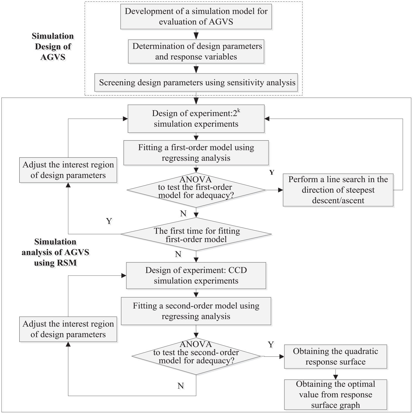
The proposed RSMSM method of optimization design of vehicle requirements of AGVS.
A detailed description of the procedures is as follows:
Establishing a simulation model of AGVS based on DES
The increased complexity of manufacturing systems makes analytical models inefficient while DES has been found as an effective tool to solve such design problems. The simulation model of AGVS is developed using simulation packages such as Arena, PlantSimulation, Flexsim, Simio, and so on. The parameters and variables of AGVS can be configured and the random variables are set. Secondary developed software is used to control the operation logic of AGVS.
Determining the design parameters and response variables
Design parameters and system performance response variables (indicators) are determined according to the specific application scenarios. The main response variables include makespan, throughput, vehicle utilization, traffic congestions/conflictions, the handling cost/times, average cycle time etc. The design parameters of AGVS include the number, speed and acceleration of AGV, the loading and unloading time of AGV, the battery charging threshold of AGV etc. Other non-ontology parameters (such as guide-paths, idle-vehicle positioning, number and location of pick-up and delivery points, AGV maintenance strategy, part arrival time, and processing routes) are used as operational parameters to run the simulation experiments. Obviously, relationships between response variables and design parameters and relations between two response variables are highly coupled and might be difficult to predict. The more the design parameters, the coupled relationships are more complex.
Screening the design parameters using sensitivity analysis
To separate sensitive parameters from the relatively stable design parameters, we can use the sensitivity analysis of simulation design to analyze the influence effect of design parameters on response variables. We change only one design parameter at a time when keeping others constant, and observe the response variable’s behavior in the simulation model to analyze the sensitivity of the parameter. All relevant design parameters are observed and screened during the sensitivity analysis. The design parameter with weak sensitivity and effect are selected as fixed parameters and used for the simulation model, while the design parameters with strong sensitivity and effect are chosen as sensitive parameters for building the valid model. Then, the equation (1) can be established after the parameters are screened and the response variables are determined with a reduced number of design parameter variables, making the problem easier to solve.
Experimental design and RSM method
RSM is an optimization method that was introduced in the early 1950s by Box and Wilson. 21 The application of RSM method in manufacturing system can be referred to the literatures (Assid et al., 22 Yang and Tseng, 23 Zhang et al., 24 Sajadi et al., 25 Thangavel et al., 26 Jahanbakhsh et al. 27 ). The RSM method based on FFD and regression analysis is used to fit the approximate function between design parameters and response variables. Usually, the first-order linear model is used for preliminary fitting. The approximate first-order model can be expressed as follows:
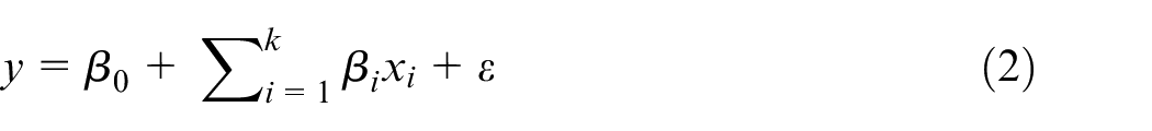
Where y denotes the response variable, β i (1 ≤ i ≤ k) represents the coefficients of main effects, and xi (1 ≤ i ≤ k) denotes the ith input variables. β0 is a constant, and ε is a random value that denotes a fitting error. A 2k experimental design with five center points is used to construct the metamodel and estimate coefficient β i .
Next, when the first-order model climbs rapidly to the optimization region along the steepest descent/ascent path, then, the second-order model is used for fitting to obtain the optimal value. The approximate second-order model can be expressed as follows:
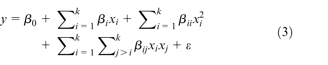
Where β ii (1 ≤ i ≤ k) denotes the coefficients of square effects, β ij (1 ≤ i,j ≤ k) denotes the coefficients of interaction effects, and xj (1 ≤ j ≤ k) denotes the jth input variable.
There are two main types of response surface designs: Box-Behnken design (BBD) and Box-Wilson Central Composite Design (CCD). BBD is an independent quadratic design and does not contain an embedded factorial or fractional factorial design. Comparing with BBD, the CCD contains an imbedded factorial or fractional factorial design with center points that is augmented with a group of “axial points” that allow estimation of curvature. BBD often has fewer design points and can be less expensive to do than CCD with the same number of factors. However, because BBD does not have an embedded factorial design, it is not suited for sequential experiments. On the contrary, CCD is especially useful in sequential experiments because the user can often build on previous factorial experiments by adding axial and center points. BBD can’t include runs from a factorial experiment, it always has three levels per factor, unlike CCD which can have up to five. Also unlike CCD, BBD never includes runs where all factors are at their extreme setting, such as all of the low/high settings. In general, CCD can better fit the quadric surface than BBD, so taken together, we adopt CCD and the results of CCD experiments are also very good.
The FFD uses the central composite design (CCD) to obtain a second-order regression model. The CCD experimental points are composed of: (1) a 2k factorial with levels coded as +1 and −1. (2) 2k axial point at coded distances ±a. (3) center points replicated n0 times. The statistical analysis of the simulation data is carried out by using the statistical software DesignExpert to obtain the coefficients of regression models and perform analysis of variance (ANOVA) to test the adequacy of these models. For more details about the implementation of RSM, please refer to the literatures (Yang and Tseng, 23 Sajadi et al., 25 Montgomery 28 and Nicolai et al. 29 ).
Computational experiments on an industrial case study
The case study
In order to evaluate the performance of the proposed method, computational experiments on an industrial case study are carried out. The simulated system in Figure 2 is modeled using PlantSimulation14.2.
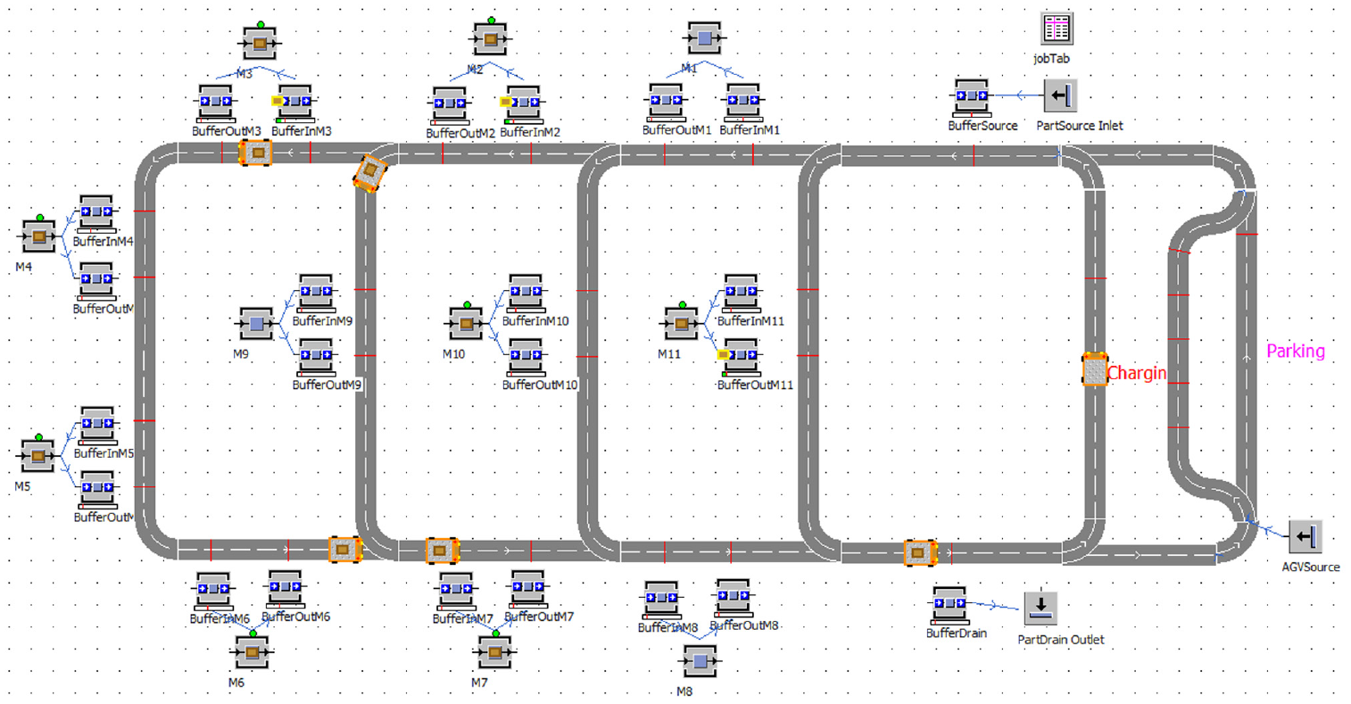
The simulation model of AGV system.
The simulation model consists of:
(1) Eleven Machining Centers (MCs) with input and output buffers.
(2) Parts inlet and outlet with incoming and outgoing buffers.
(3) AGV system with fixed unidirectional guide paths.
(4) AGV system is equipped with charging and parking station.
The assumptions and limitations applied for the model development are as follows:
(5) MCs and AGVs operate continuously without breakdown.
(6) Each MC can process only one operation for one part at a time.
(7) Each part, once started, must be processed to complete.
(8) Each AGV can carry only one part at a time.
(9) Dispatching rule for the AGVs or parts is the closest rule.
(10) The deadlock of AGV is not considered since the guide-paths are unidirectional.
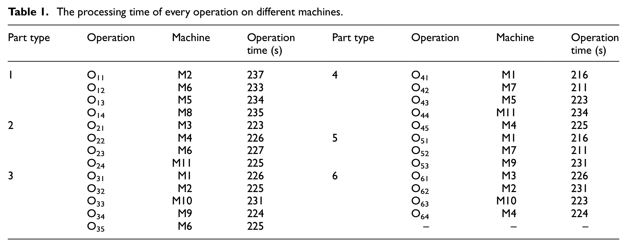
Parts enter the system from incoming buffer located in inlet, a total of 300 parts arrive randomly according to the time interval of distribution normal (4:30,30) in the sequence from 1 to 6 type and 2 parts arrive for each type every time. The process route for six types of part is shown in Table 1. The AGVs move parts among the buffers of inlet, MCs and outlet. The AGVs can go to the parking area for its idle state, or the charging area for charging when the battery power of AGV is lower than AGV charging threshold. The part will leave the system from the outgoing buffer located in outlet when the part processing is completed.
The processing time of every operation on different machines.
Simulation analysis by the proposed RSMSM method
Design parameters and response variables for the AGV system
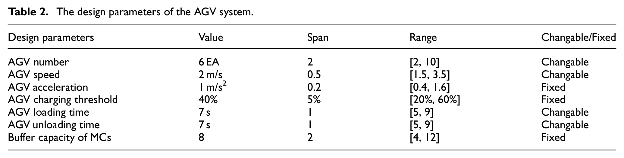
The response variables and design parameters need to be defined first for the vehicle requirements of AGVS. we consider the makespan and AGV utilization, which are the most fundamental for evaluation of system efficiency. Table 2 presents the specification of the design parameters considered in this case study: AGV number, AGV speed, AGV acceleration, AGV charging threshold, AGV loading time, AGV unloading time and buffer capacity of MCs. The constraint range and starting point value of the parameters are determined according to the expert experience.
The design parameters of the AGV system.
Sensitivity analysis for the AGVS model
We define the design parameter’s span for the sensitivity analysis, as shown in Table 2. Several simulation experiments are carried out to analyze the sensitivities of the response variables to all design parameters and initially validate the model.
Figure 3 shows that the AGV charging threshold, AGV acceleration and buffer capacity hardly have an effect while the other four parameters affect the response variables. The result shows that AGV number and AGV speed correlate with AGV utilization and makespan negatively, AGV loading/unloading time correlate with AGV utilization negatively, and correlate with makespan positively. The values for the makespan and utilization are normalized to present in the absolute value range [0,1]. Therefore, we divide the design parameters into four sensitive changable parameters and three fixed parameters as shown in Table 2.
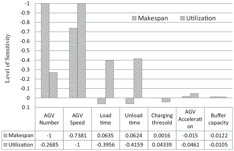
Sensitivity analysis of the design parameters for the response variables.
Mathematical model for the AGVS model
According to the above analysis, the changable design parameters are the number of AGV(x1), the speed of AGV(x2), the unloading time of AGV(x3) and the loading time of AGV(x4). The response variables include the AGV utilization (y1) and makespan (y2), which can be expressed as follows:
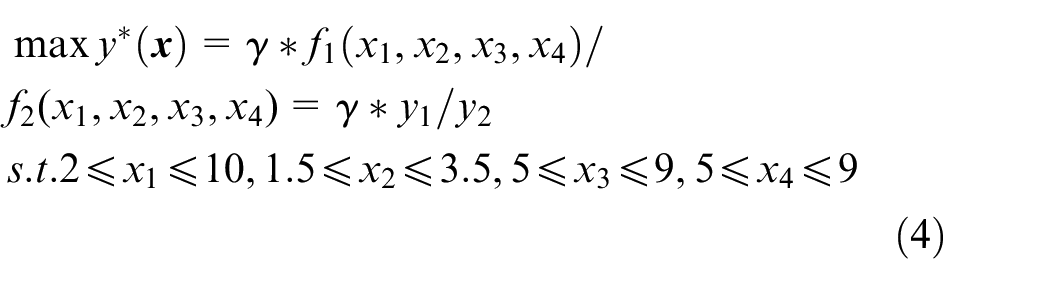
where x1 is a discrete variable, x2, x3, and x4 are continuous variables, γ = 10E + 06 is the coefficient of ratio, reflecting the equal weights for y1 and y2 and relative size of y1 and y2.
Experimental design and analysis by RSM method
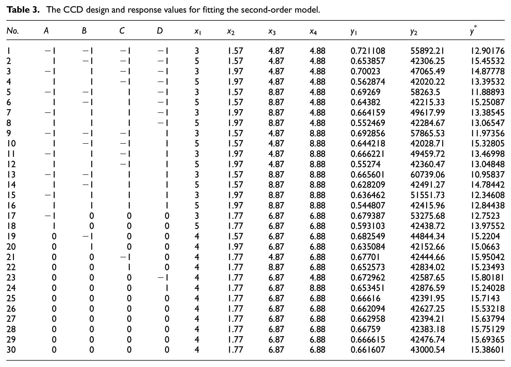
According to the procedure of RSM method, a first-order model described in equation (2) is first fitted from center points (x1 = 6, x2 = 2, x3 = 7, x4 = 7), and a linear search is performed in the direction of steepest ascent. Then it reaches a new center point (4, 1.77, 6.87, 6.88), the result of new experiments denotes the new first-order model is not adequate and the curvature and interaction are found to be quite evident. So, a second-order model described in equation (3) is needed to fit the response value, we augment the 2 k factorial design with n0 = 6 central runs and 2k = 8 axial runs with a = ±1. a is the distance of the axial points from the design center. This CCD is rotatable and provides equal precision of estimation in all directions. Table 3 shows this design and related response values. A,B,C,D are coded variables corresponding to the natural variables x1, x2, x3, x4 one by one. Each of the experiment case is simulated for five independent replications.
The CCD design and response values for fitting the second-order model.
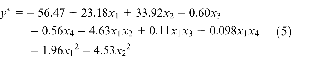
Then the second-order model described in equation (3) is used to fit the response value y* by DesignExpert, and ANOVA is used to test the model for adequacy. The significance level of F-test is α = 0.05. If the value of “p value” is less than 0.05, then the corresponding term is significant. Otherwise, if the value is greater than 0.10, then the corresponding term is not significant. The non-significant terms in the model are eliminated and the model should be re-fitted. Finally we get a reduced model, the resulting reduced equation of the fitted second-order model is as follows:
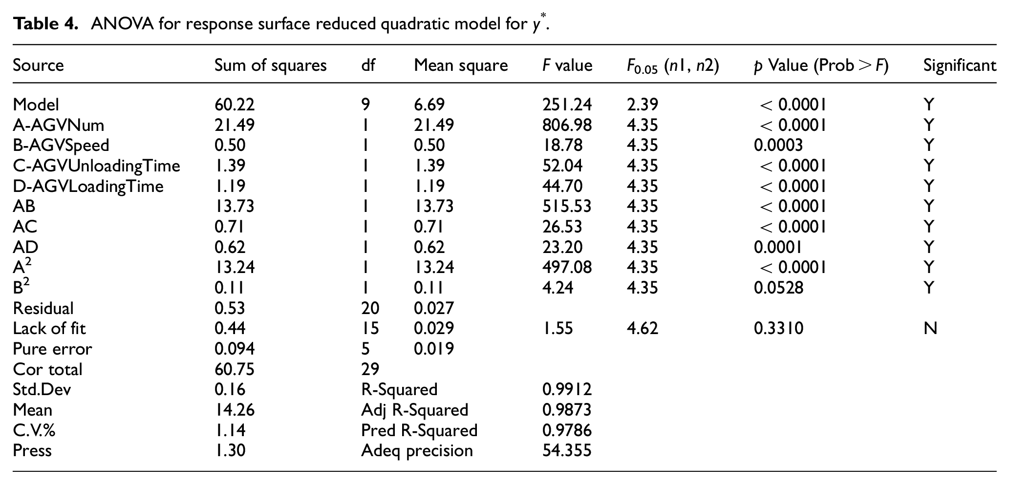
The summary results of ANOVA for the reduced model are generated in Table 4, and the adequacy of the second-order model is investigated. The overall regression F-test of the second-order model is significant while the lack of fit test is non-significant. Meanwhile, the “Pred R-Squared” of 0.9786 is in reasonable agreement with the “Adj R-Squared” of 0.9873, so the above regression model is adequate and equation (5) is fitting the data well.
ANOVA for response surface reduced quadratic model for y*.
In addition to the numerical analysis, DesignExpert also generates a graphical presentation to investigate the fitted model. Response surface diagrams of significant interaction factors given by DesignExpert are shown in Figure 4. The contour and 3D plot analysis can be performed to obtain the optimal value from the response surface graph.
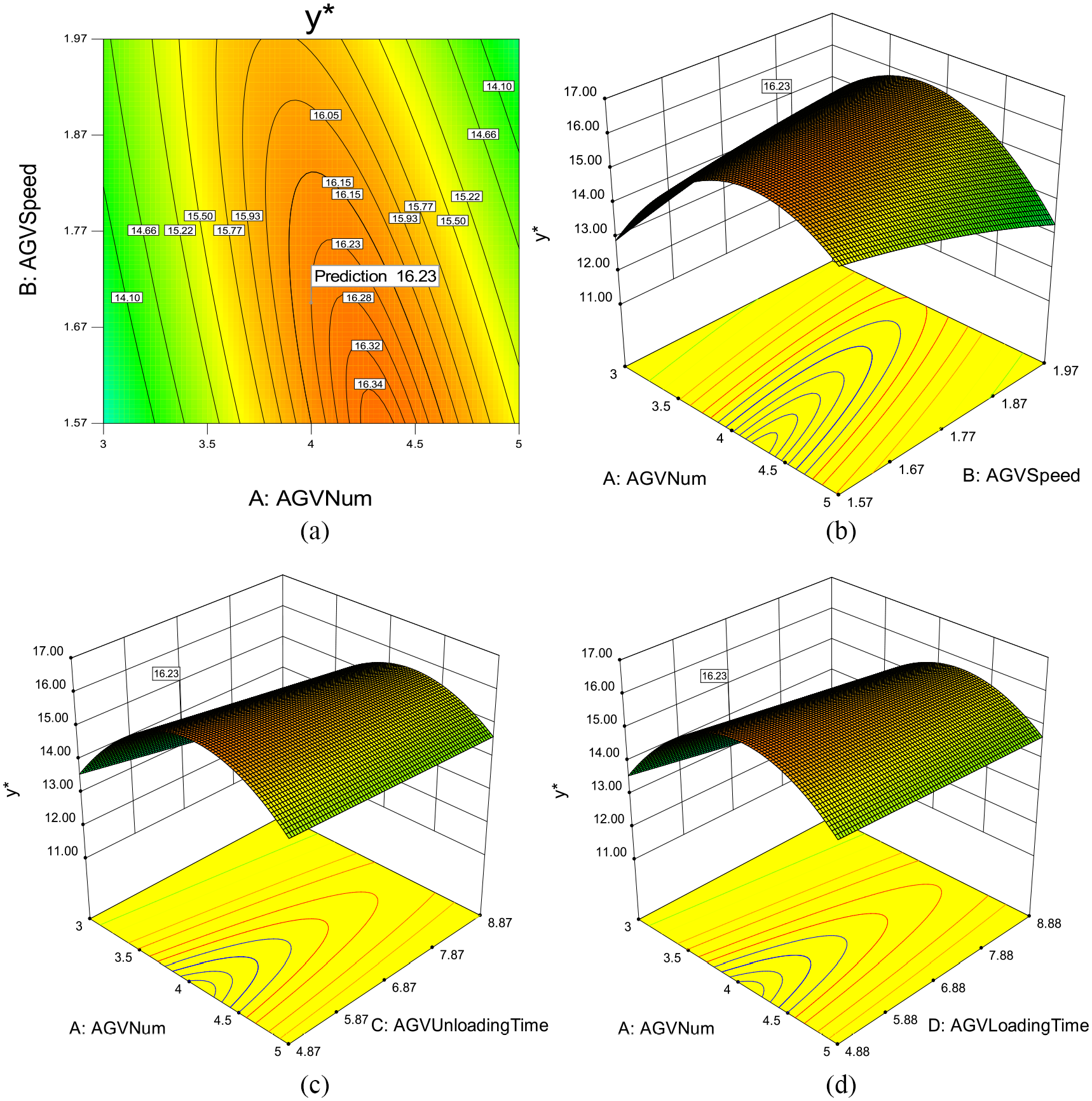
Response surface diagrams of significant interaction factors: (a) contour plot for y* (A-B), (b) 3-D plot for y*(A-B), (c) 3-D plot for y* (A-C), and (d) 3-D plot for y*(A-D).
The interactions of the four factors (AGVNum, AGVSpeed, AGVUnloadingTime, and AGVLoadingTime, denoted as A, B, C, D) can be described as follows: significant interaction factors include A-B, A-C, and A-D, while the interactions of B-C, B-D, and C-D are not significant. As can be seen from Figure 4(b), when the value of A is fixed, the value of y* increases with the decrease of B, it can be inferred from Figure 4(c) and (d) that C and D also have the same effect as B. From Figure 4(a) and (b), the optimal region shown in the 3-D plot implies a stable optimal region, the area surrounded by the contour line of 16.23 denotes the approximate region of the optimal y*. Therefore, considering the number of AGVs is a discrete number value, the optimal solution can be chosen as x1 = 4, x2 = 1.69, x3 = 5, x4 = 5. The expected maximum value of y* at the chosen point is 16.23.
Comparison verification with GA-based/PSO-based simulation optimization method
GA-based/PSO-based simulation optimization method for vehicle requirement of AGVS simulation model
Genetic Algorithm (GA) is a heuristic method based on natural selection and genetics. Due to its efficient and robust performance, GA has been employed in conjunction with simulation in some manufacturing environments, which is called GA-based simulation optimization method. Many researchers apply GA-based simulation optimization method in determining some optimum conditions in complex manufacturing systems. See related literatures (Jeong et al., 30 Lee and Kim, 31 Gholami and Zandieh, 32 Zhang et al. 33 ). GA-based simulation optimization is employed to find the optimal parameters and determine the best set of response values of the above AGV simulation model. We use GAWizard toolbox in PlantSimulation to perform the GA-based simulation optimization. The operating parameters of GA are as follows: The number of generations is 15, the size of generation is 20; The optimization parameters include x1, x2, x3, x4 as described in equation (4), fitness function is y*; three observations per individual, crossover probability is 0.8, mutation probability is 0.1. Figure 5 presents the progress of GA simulation optimization for y*. As the optimization makes more runs, the response value becomes about 16.40 and all lines converge, indicating that this is the best solution it can find.
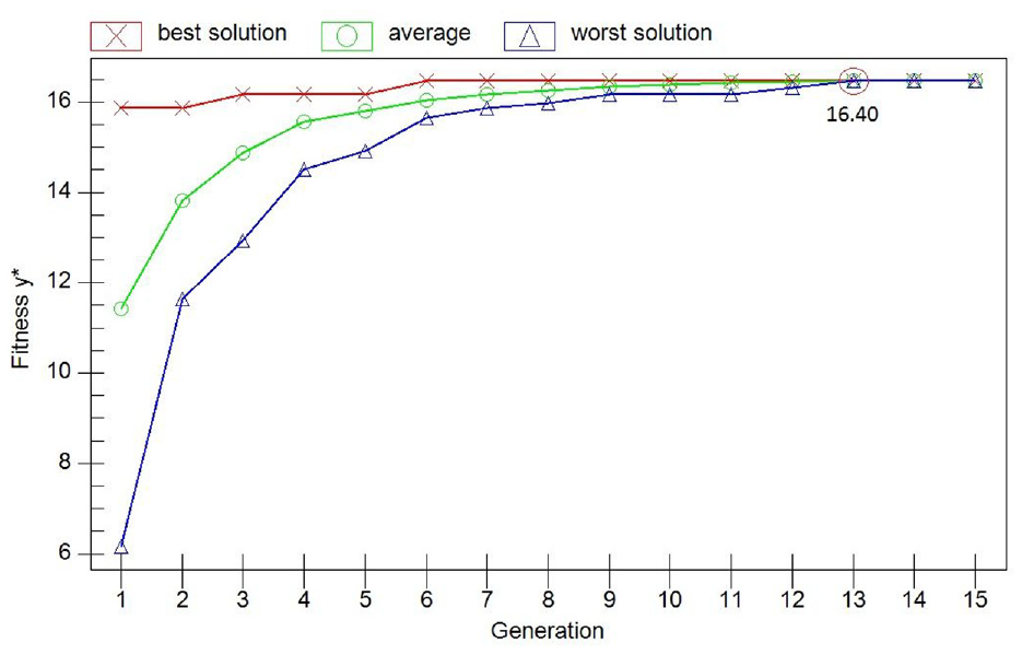
GA-based simulation optimization progress for y*.
In order to further confirm the feasibility of the proposed method in this paper, we adopt another method called PSO-based simulation optimization to carry out the comparative experiment again. The method combines PSO with DES and can be used to solve some optimization problems in manufacturing system. See related literatures (Phatak et al., 34 Liao and Lin 35 ). We apply PSO as our searching algorithm for optimization and apply simulation software (PlantSimulation) to evaluate performance or fitness. The operating parameters of PSO are as follows: The number of generations is 24, the size of generation is 20; the inertia weight is 0.8, the cognitive constant is 0.5 and social constant is 0.5, three observations per individual. Figure 6 presents the progress of PSO simulation optimization for y*. As the optimization makes more runs, the response value becomes about 16.44 and all lines converge, indicating that this is the best solution it can find.
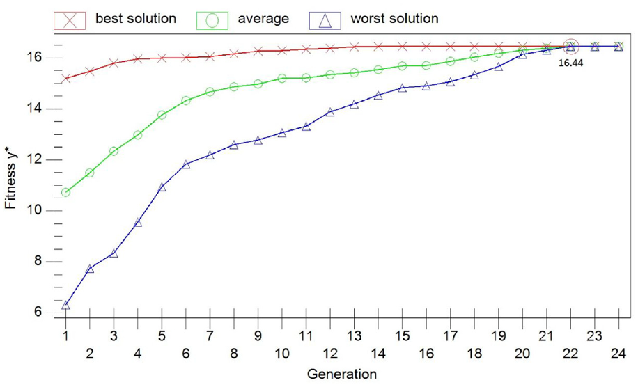
PSO-based simulation optimization progress for y*.
Results and validation test between RSMSM and GA/PSO
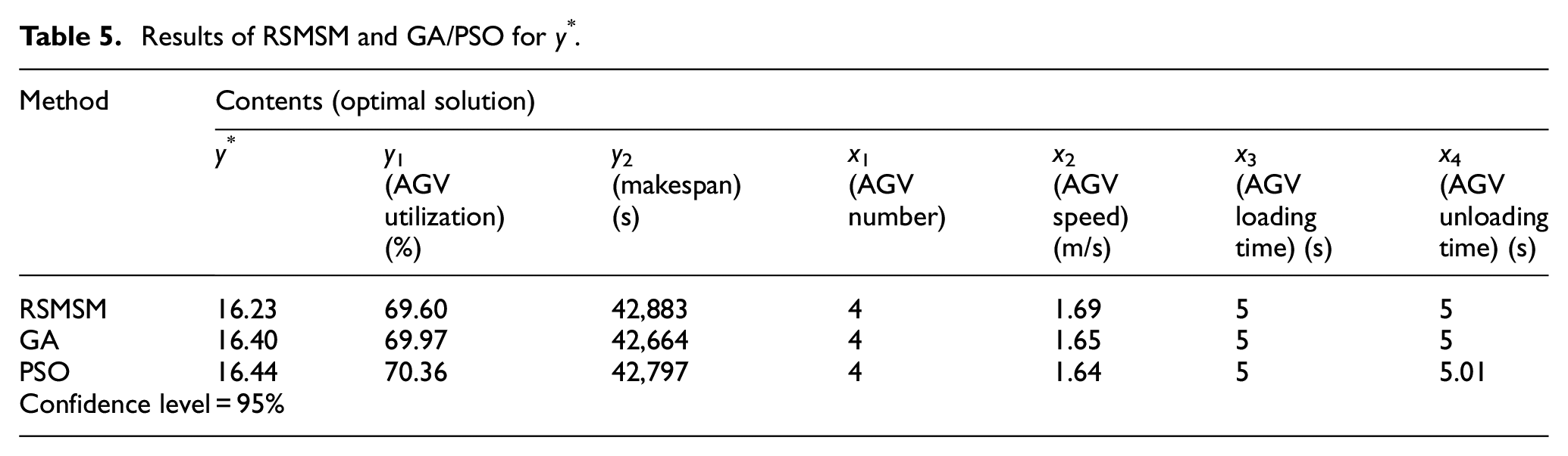
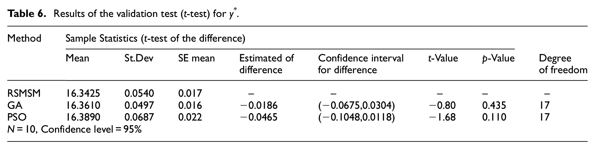
The results of RSMSM and GA-based/PSO-based simulation optimization are summarized in Table 5, it seems that there is no large difference between the methods. In order to establish this with certainty, we carry out a validation test introduced in Um et al. 13 to employ a t-test to detect the difference between result datasets of different methods. Then, the retrial is executed for each RSMSM and GA/PSO with 10 replications to construct the datasets for the t-test. The results of t-test are presented in Table 6. First consider the comparison between RSMSM and GA, the estimate of the difference value (−0.0186) falls within the confidence interval for the difference (−0.0675, 0.0304), the p-value (0.435) is greater than the significance level (α = 0.05). It indicates the absence of any obvious difference of means for the two samples. So we can conclude that there is no statistically significant difference between the two methods in the design parameters and response variables. Then consider the comparison between RSMSM and PSO, we can reach the same conclusion.
Results of RSMSM and GA/PSO for y*.
Results of the validation test (t-test) for y*.
In addition to the comparison of solution results, the number of experiments between the RSMSM method and GA/PSO method are also compared. The GA method generates 458 evaluated individuals, it means that 458 simulation experiments need to be performed. The PSO method needs to carry out 475 simulation experiments. The number of experiments required by RSMSM method is the sum of the three rounds of experiments, which is 21 + 21 + 30, so 72 simulation experiments need to be done. It can be seen that RSMSM method can greatly reduce the number of simulation experiment runs.
Conclusion
In this paper, we first review and analyze the AGVS vehicle requirements problem and define the problem as an optimization problem, then a simulation-based analytic methodology named RSMSM is presented. The RSMSM method combines DES, sensitivity analysis, FFD and RSM components. A numerical example is developed to verify the proposed method by comparing it with GA-based/PSO-based simulation optimization method. Finally, we can come to the following conclusion:
(1) Sensitivity analysis carried out for AGV design parameters indicates that AGV number and AGV speed have the greatest influence on the performance of manufacturing system, followed by AGV loading/unloading time, while the AGV acceleration, AGV charging threshold, etc. have no obvious influence. Sensitivity analysis can filter out unimportant parameters early and reduce the complexity of the problem model.
(2) From a statistical point of view, the RSMSM method can get basically the same optimal solution when compared with GA-based/PSO-based simulation optimization method. However, the RSMSM method can reduce the number of simulation experiments by more than 80% in our case study. The reason lies in that the RSM can quickly climb to the optimal region in the first-order model fitting stage, thus can reduce the redundant simulation experiments in the non-optimal region. This advantage can reduce cost and improve efficiency in practical engineering application.
(3) The method combines the simulation method with analytical method, which can make a full use of their respective advantages and overcome the defects of existing methods. Simulation can retain the system’s authenticity to the greatest extent and reduce the deviation of the problem model. Meanwhile, the quadratic polynomial fitting mathematical model based on FFD simulation test is simple in form and easy to solve in general.
Although the RSMSM method is very practical, but not perfect. In general, the RSM is a local search method, which performs well in a relatively small area. When a searching region is too large, the method may easily fall into local optimum. Therefore, other methods could be combined with RSMSM to avoid falling into the local optimum. In addition, other factors such as AGV/machine scheduling rules, job sequencing, task level, flowpath layout, positioning of idle vehicles, etc. are not yet considered, which also affect design parameters and response variables. In the next step, we will consider these two points for a more comprehensive study.
Footnotes
Appendix
Declaration of conflicting interests
The author(s) declared no potential conflicts of interest with respect to the research, authorship, and/or publication of this article.
Funding
The author(s) disclosed receipt of the following financial support for the research, authorship, and/or publication of this article: This research is supported by the Major State Basic Research Program in Sichuan Province of China (Grant number 20YYJC4377).