Sage Journals: Discover world-class research

Abstract

Cutting tool wear prediction plays an important role in the machining of complex aerospace parts, and it is still a challenge under varying cutting conditions. To overcome the limitations of the existing methods in generalization ability when dealing with cutting conditions changing largely, this paper proposed a novel cutting tool wear prediction method based on continual learning. A meta-LSTM model is firstly trained for specific cutting conditions and can be easily fine-tuned with very small number of samples to adapt to new cutting conditions. Specifically, the meta-model could be continuously updated as machining data increase by using an orthogonal weights modification method. The experiment results show that the proposed method can realize accurate prediction of tool wear under different cutting conditions. Compared with existing methods including meta-learning methods, the range of adapted cutting conditions could be expanded as the task distribution of new cutting conditions is continuously learned by the prediction model.

Keywords

NC machining tool wear data-driven prediction continual learning

Introduction

With the introduction of “Industry 4.0” in Germany, the fourth industrial revolution led by intelligent manufacturing has been launched globally. As a key technology in the manufacturing field, Numerical Control (NC) machining has more and more requirements in automation and intelligence. Online prediction of cutting tool wear is an important part to realize the automation and intelligence in machining process. Especially in production lines, in order to ensure production continuity to improve production efficiency and ensure processing quality, it requires higher level of automation and intelligence, and the online prediction of cutting tool wear is much more urgent.

With the development in aerospace industry, difficult-to-cut materials such as titanium alloys and high-temperature alloys have been widely used in aerospace complex parts. During the machining process of the parts, cutting tool wear is more serious,¹ and the cutting tool may even be broken, which may significantly impact surface texture or machining precision.² In practice, cutting tools are changed more often than necessary because it is difficult to accurately predict tool wear. For example, over 40 cutting tools are needed to complete the milling of nickel-based superalloy part³ and only 50%–80% of cutting tool life is rationally used.⁴ On the other hand, the new generation aerospace products have higher requirements in machining accuracy and surface quality to satisfy the high performance, accompanied with higher requirements of tool wear prediction accuracy. For example, considering the tool wear rate is 0.009 mm/min under a certain cutting condition, if the prediction accuracy is 0.09 mm and it is equivalent to the tool wear value with 10 min cutting process, while it is under high risk for the cutting tool to be up to the wear limitation during the process, as it always takes about 10 min to process a machining feature. Under some cutting conditions with more rapid tool wear or with higher surface quality, higher prediction accuracy is required. Furthermore, in some complex cutting conditions such as corner milling during cutting large–sized parts, tool wear is more difficult to predict and unexpected over worn or broken situations may occur during the cutting process, which may cause part failure. As reported, during the machining of a structural part with the material of titanium alloy in an aerospace manufacturing enterprise, severe tool wear caused the workpiece ablated and scrapped due to non-prediction of tool state in time. Therefore, accurate online prediction of cutting tool wear is crucial for ensuring machining quality and reducing cost during machining process, especially for large-sized and difficult-to-cut materials used in airplanes.

This paper proposed a novel method for accurately predicting cutting tool wear under different cutting conditions based on continual learning for cutting in NC machining. Cutting tool wear under a specific cutting condition could be predicted by Long Short Term Memory (LSTM) as a base-model. Model-Agnostic Meta-Learning (MAML)⁵ is used to update the meta-model parameters of the LSTM to adapt different cutting conditions. After the meta-LSTM model is successfully trained, the model can be easily fine-tuned with very small number of samples so as to adapt to new cutting conditions. Specifically, the meta-model, incorporating efficient and scalable continual learning, could be continuously updated by new cutting conditions during the machining process, that is, learning different tasks sequentially, one at a time. The meta-parameters are fine-tuned by orthogonal weights modification method with small samples in new cutting conditions. Compared with existing meta-learning methods, the range of adapted cutting conditions could be expanded as the task distribution of new cutting conditions is continuously learned by the prediction model.

Related works

There have been plenty of reported studies on cutting tool wear prediction. Previous research aimed to predict tool wear using tool wear mechanism modeling methods.^6–12 For example, Rech et al.¹⁰ proposed a tribological approach to predict cutting tool wear. It identified a fundamental wear model using a dedicated tribometer, and it is able to simulate relevant tribological conditions encountered along the tool–work-material interface. However, tool wear during machining is a complex physical and chemical process, while traditional model can only consider some specific processes such as friction and deformation. During the considered specific processes, tool wear is influenced by many factors, and traditional models can only consider some specific factors, such as cutting temperature, cutting force, material of cutting tool and so on, even in this situation, the tool wear process can only be modeled by significant simplification and assumptions, while the solution searching procedure is still complex, and can only be obtained by approximation. So traditional prediction methods are not accurate, and can only predict tool wear stages in the whole tool life.

Due to the complexity of tool wear during machining process, the establishment of tool wear mechanism models is more and more challenging, while data-driven methods can learn data-driven models from a large volume of data, and the data-driven model can be equivalent to complex mechanism models within certain range of error, so data-driven method provides a new idea for accurate tool wear prediction.^13–18

Some existing data driven methods such as deep learning have been used to predict cutting tool wear.^19–21 For example, Zhao et al.²⁰ proposed a deep learning method for tool wear prediction. The Convolutional Bi-Directional LSTM Networks were established and the convolutional neural network was used for feature extraction while the LSTM network was used for tool wear monitoring. Shi et al.²¹ established two deep auto-encoder networks, one for signal feature extraction and another one for tool wear prediction in the given cutting condition. Deep learning has limitations in varying cutting conditions, because it needs to be trained on different cutting conditions with a large number of labeled samples which have to include monitoring signals and corresponding tool wear label. Considering the multi-dimensional input space and the complex structure of deep network for tool wear prediction, the training samples needed by deep learning may be 10,000 or 100,000. However, in actual machining area, labelled samples are difficult to obtain. The experiments for obtaining samples are time consuming and costly, each label of the cutting tool wear should be measured with a series of sophisticated operations by interrupting machining process. So it is impossible to train a perfect deep learning model for predicting tool wear under all cutting conditions.

In order to overcome the limitations of large number of labelled samples needed by deep learning, a meta-learning method for tool wear prediction was proposed by the authors Li et al.²² Different base-models are trained over specific tasks, as each base-model for a specific cutting condition should not be very complex, and the sample requirement is not large, so each base-model is easy to train. A meta-learning model can be trained during the training process of base-models, where the meta-learning model can learn the natural law of the change of base-models, and the meta-learning model can be easily adjusted so as to adapt to new cutting conditions. In this case, the required training samples are significantly reduced compared with deep learning which tries to train a complex model.

However, if the cutting conditions change largely (e.g. the cutting parameters or diameter of cutting tools are quite different), the prediction accuracy of meta-learning may decrease, because the generalization ability is limited by the task distribution of base-models for different cutting conditions.²³ This point should be developed further more.

Cutting tool wear prediction method based on continual learning

Approach overview

The overall idea of the proposed tool wear prediction method is shown in Figure 1. A base-model is a LSTM to predict tool wear under a specific cutting condition by taking advantages of the time series of Recurrent Neural Network (RNN), where the cutting tool wear rule can be implicitly learned. The inputs of LSTM are signal features of vibration, power and current, which are preprocessed by entropy weight-grey correlation analysis²² and manifold learning. MAML⁵ is used to update the meta-model parameters of the LSTM to adapt different cutting conditions. After the meta-LSTM model is successfully trained, the model can be easily fine-tuned with very small number of samples so as to adapt to new cutting conditions. Specifically, the meta-model, incorporating efficient and scalable continual learning, could be continuously updated by new cutting conditions during the machining process, that is, learning different tasks sequentially, one at a time. The meta-parameters are fine-tuned by orthogonal weights modification method with small samples in new cutting conditions. Compared with existing meta-learning methods, the range of adapted cutting conditions could be expanded as the task distribution of new cutting conditions is continuously learned by the prediction model. Such an ability is crucial to humans as well as artificial intelligence agents for two reasons: (1) there are too many possible cutting conditions to learn concurrently, and (2) useful mappings cannot be pre-determined but should be learned when corresponding cutting conditions are encountered.

Figure 1.

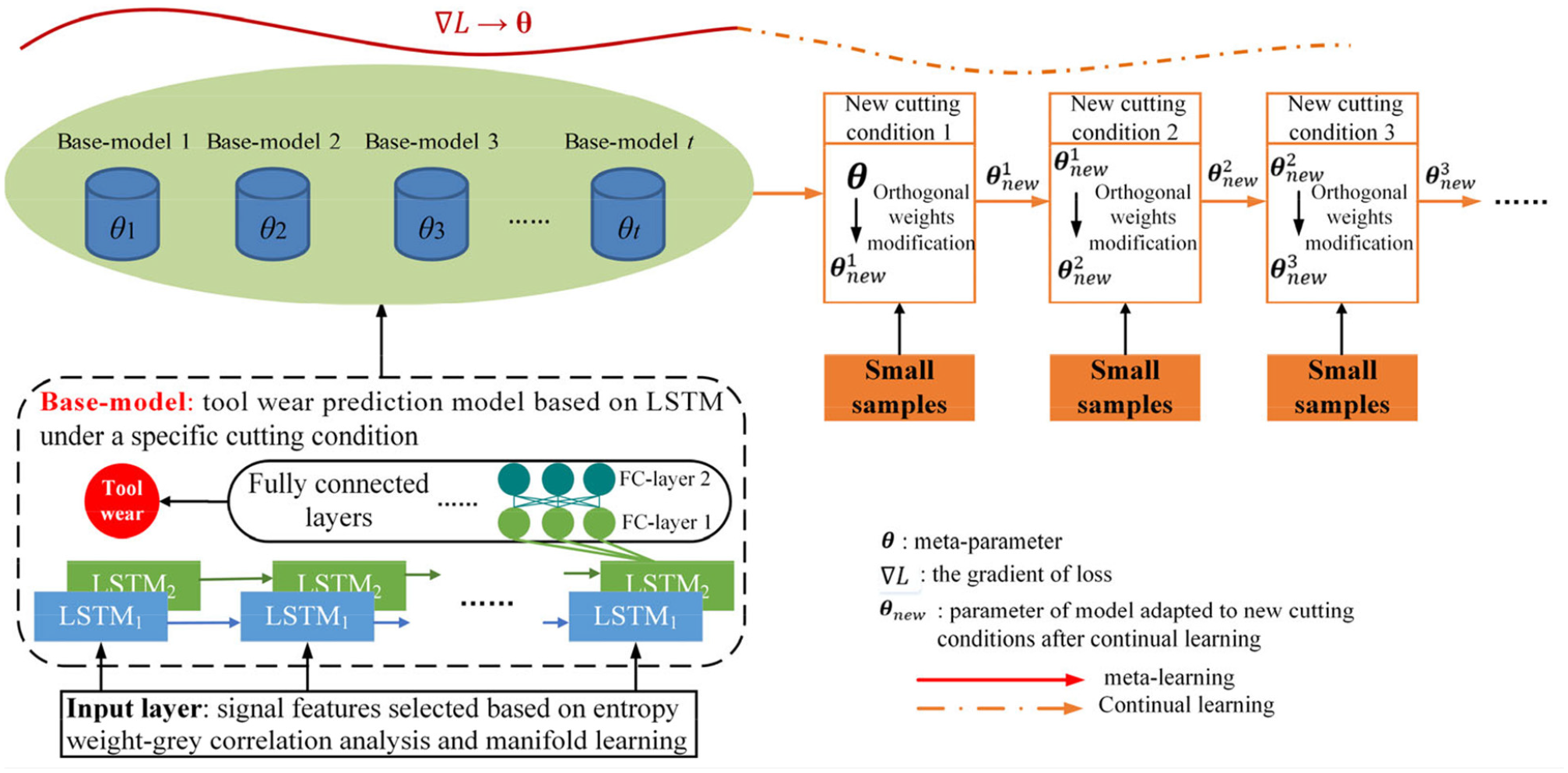
The overall idea of the proposed tool wear prediction method.

Continual learning for cutting tool wear prediction based on orthogonal weights modification method

The main idea of continual learning is learning different tasks sequentially, one at a time. So the continual learning method could update the meta-model parameters by new cutting conditions, while the meta-learning model is constant after successfully trained in meta-learning method. Compared with existing meta-learning methods, the range of adapted cutting conditions could be expanded as the task distribution of new cutting conditions is continuously learned by the prediction model. Such an ability is crucial to humans as well as artificial intelligence agents.

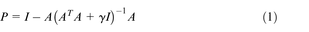
The main obstacle to achieve continual learning is that conventional neural network models suffer from catastrophic forgetting, that is, training a model with new tasks interferes with previously learned knowledge and leads to significant decreases in the performance of previously learned tasks.^24,25 To avoid catastrophic forgetting, the orthogonal weights modification method²⁶ is used for continual learning. Specifically, when the tool wear prediction model is adjusted for new cutting conditions, the feature space of its parameters can only be modified in the direction orthogonal to the subspace spanned by all previously learned inputs, as shown in Figure 2. This ensures that new learning processes do not interfere with previously learned tasks, as model parameter changes in the network as a whole do not interact with old inputs. Consequently, combined with a gradient descent-based search, the orthogonal weights modification method helps the prediction model to find a weight configuration that can accomplish new tasks while ensuring the performance of learned tasks remains unchanged. This is achieved by constructing a projector used to find the direction orthogonal to the input space, represented as formula (1):

Figure 2.

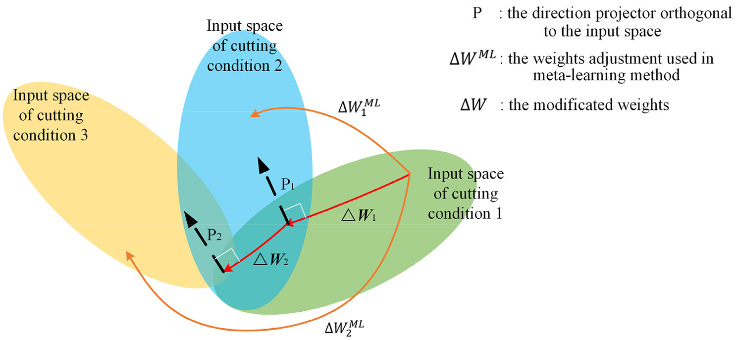
The representation of the orthogonal weights modification method in tool wear prediction model.

P = I - A {(A^{T} A + γ I)}^{- 1} A

(1)

where matrix $A$ consists of all previously trained input vectors as its columns $A = [x_{1},' \dots, x_{n}]$ , I is a unit matrix multiplied by a relatively small constant $γ$ , and $A^{T}$ is the transpose of $A$ . The learning-induced modification of weights is then determined by $Δ W = κ P Δ W^{ML}$ , where $κ$ is the learning rate and $Δ W^{ML}$ is the weights adjustment calculated according to the standard backpropagation, which is used in meta-learning method.

In the (i+1)th task, the tool wear prediction model is adjusted by orthogonal weights modification method according to formula (2):

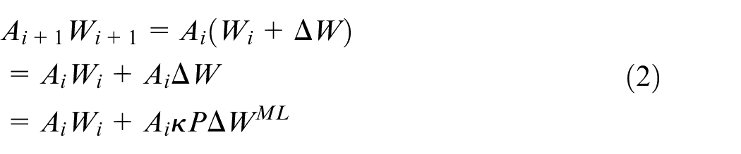
\begin{matrix} A_{i + 1} W_{i + 1} = A_{i} (W_{i} + Δ W) \\ = A_{i} W_{i} + A_{i} Δ W \\ = A_{i} W_{i} + A_{i} κ P Δ W^{ML} \end{matrix}

(2)

The input space is orthogonal to the projector P, so the second term of the right-hand formula is equal to 0. This means that new learning processes do not interfere with previously learned tasks.

To calculate P in formula (1), an iterative method can be used. Specifically, consider a neural network of L+1 layers, indexed by l=0, 1, 2, …, L with l = 0 and l = L being the input layer and output layer, respectively. All hidden layers share the same activation function g. $W_{l}$ represents the connections between the (l−1)th and lth layer with $W_{l} \in {' R}^{s \times m}$ . x _l and y _l represent the input and output of the lth layer, respectively, where x _l = g( y _l) and y _l = $W_{l}^{T} x_{l - 1}$ . $x_{l - 1} \in {' R}^{s}$ and $y_{l} \in {' R}^{m}$ , where s and m are the dimension of input and output, respectively.

In the orthogonal weights modification method, the orthogonal projector P_l defined in the input space of layer l for learned tasks (cutting conditions that the model has encountered) is key for overcoming catastrophic interference in continual learning. In practice, P_l can be recursively updated for each task in a way similar to calculating the correlation-inverse matrix in the recursive least square (RLS) algorithm,^27,28 as shown in formula (3):

P^{(RLS)} = {(\sum_{i = 1}^{n} x (i) x^{T} (i) + γ I)}^{- 1}

(3)

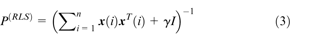
This method allows P_l to be determined based on the current inputs and the P_l for the last task. It also avoids matrix-inverse operation in the original definition of P_l. The detailed procedure for the implementation of the orthogonal weights modification method is shown by Algorithm 1.

Algorithm 1: orthogonal weights modification
Require: $W_{l} (0)$ from meta-LSTM model; Require: $P_{l} (0) = \frac{I_{l}}{δ}$ for l = 1, …, L, where $δ$ is a regularization constant; Require: M: the number of batch; Require: N: the number of task 1: Forj from 1 toN, do 2: Fori from 1 toM, do 3: Propagate the inputs of the ith batch in the jth task forward 4: Propagate the errors and calculate weight modifications $Δ {W_{l}}^{ML} (i, j)$ for $W_{l} (i - 1, j)$ backward by the standard BP method 5: Update the weight matrix in each layer by $W_{l} (i, j) = W_{l} (i - 1, j) + κ (i, j) Δ {W_{l}}^{ML} (i, j)$ if j = 1 $W_{l} (i, j) = W_{l} (i - 1, j) + κ (i, j) P_{l} (j - 1) Δ {W_{l}}^{ML} (i, j)$ if j = 2, 3, … where $κ (i, j)$ is the predefined learning rate 6: End for 7: Propagate the mean of the inputs for each batch (i = 1, …, n_j) in the jth task forward successively. 8: Update $P_{l}$ for $W_{l}$ as $P_{l} (j) = P_{l} (n_{j}, j)$ , where $P_{l} (j) = P_{l} (n_{j}, j)$ can be calculated iteratively according to: $P_{l} (i, j) = P_{l} (i - 1, j) - k_{l} (i, j) {\bar{x}}_{l - 1} {(i, j)}^{T} P_{l} (i - 1, j)$ $k_{l} (i, j) = \frac{P_{l} (i - 1, j) {\bar{x}}_{l - 1} (i, j)}{γ + {\bar{x}}_{l - 1} {(i, j)}^{T} P_{l} (i - 1, j) {\bar{x}}_{l - 1} (i, j)}$ in which ${\bar{x}}_{l - 1} (i)$ is the output of the (l-1)th layer in response to the mean of the inputs in the ith batch of the jth task, and $P_{l} (0, j) = P_{l} (j - 1)$ . 9: End for

Algorithm 1: orthogonal weights modification

Require:

W_{l} (0)

from meta-LSTM model;
Require: $P_{l} (0) = \frac{I_{l}}{δ}$ for l = 1, …, L, where

δ

is a regularization constant;
Require: M: the number of batch;
Require: N: the number of task
1: Forj from 1 toN, do
2: Fori from 1 toM, do
3: Propagate the inputs of the ith batch in the jth task forward
4: Propagate the errors and calculate weight modifications

Δ {W_{l}}^{ML} (i, j)

for

W_{l} (i - 1, j)

backward by the standard BP method
5: Update the weight matrix in each layer by

W_{l} (i, j) = W_{l} (i - 1, j) + κ (i, j) Δ {W_{l}}^{ML} (i, j)

if j = 1

W_{l} (i, j) = W_{l} (i - 1, j) + κ (i, j) P_{l} (j - 1) Δ {W_{l}}^{ML} (i, j)

if j = 2, 3, … where

κ (i, j)

is the predefined learning rate
6: End for
7: Propagate the mean of the inputs for each batch (i = 1, …, n_j) in the jth task forward successively.
8: Update

P_{l}

for

W_{l}

P_{l} (j) = P_{l} (n_{j}, j)

, where

P_{l} (j) = P_{l} (n_{j}, j)

can be calculated iteratively according to:

P_{l} (i, j) = P_{l} (i - 1, j) - k_{l} (i, j) {\bar{x}}_{l - 1} {(i, j)}^{T} P_{l} (i - 1, j)

k_{l} (i, j) = \frac{P_{l} (i - 1, j) {\bar{x}}_{l - 1} (i, j)}{γ + {\bar{x}}_{l - 1} {(i, j)}^{T} P_{l} (i - 1, j) {\bar{x}}_{l - 1} (i, j)}

in which

{\bar{x}}_{l - 1} (i)

is the output of the (l-1)th layer in response to the mean of the inputs in the ith batch of the jth task, and

P_{l} (0, j) = P_{l} (j - 1)

.
9: End for

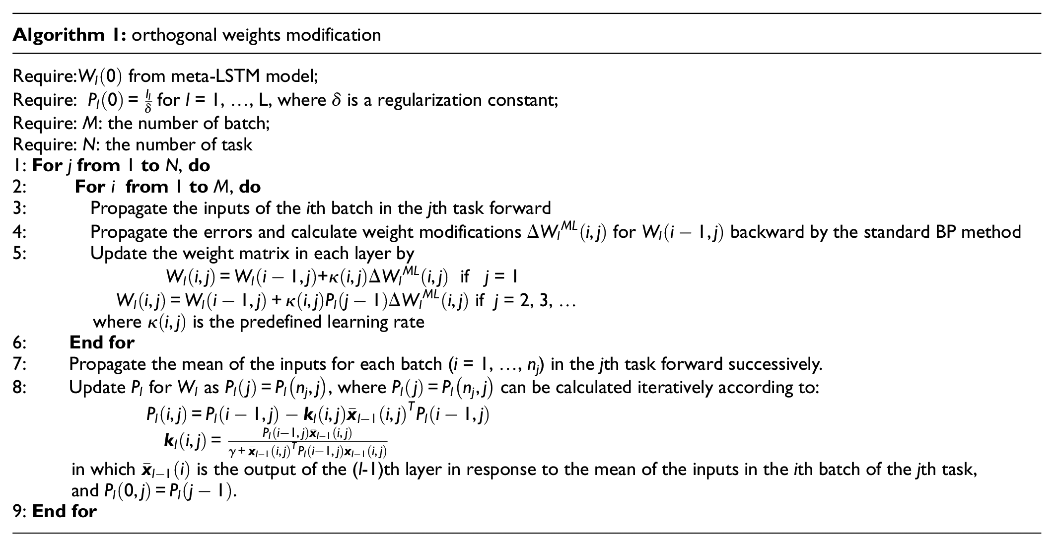
The algorithm does not need to store all previous inputs A. Instead, only the current inputs and projector for the last task are needed. This iterative method is related to the RLS algorithm, which can be used to train feed-forward and RNN to achieve fast convergence, tame chaotic activities²⁹ and avoid interference between consecutively loaded patterns or tasks.³⁰

In addition, the capacity of the orthogonal weights modification method is analyzed, i.e., how many different cutting conditions could be learned and adapted to using this method. The capacity of one network layer can be measured by the rank of P(i), which is defined as the orthogonal projector calculated after cutting condition i, with ΔP(i+ 1) then defined as the update in the next cutting condition satisfying P(i+ 1) = P(i) –ΔP(i+ 1). As range $(P (i + 1)) \cap^{} (Δ P (i + 1)) = \emptyset$ , rank(P(i+ 1)) = rank(P(i)) – rank(ΔP(i+ 1)). In the ideal case where each task consumes the capacity effectively, as the learning process continues, the rank of $P_{l}$ is approaching 0, indicating that this particular layer no longer has the capacity to learn from new cutting conditions. The capacity of the whole network can be approximated by the summation of the capacity of each layer, as shown in formula (4):

ran k_{tot} = \sum_{l = 1}^{L} \frac{rank (P_{l})}{rank (δ I_{l})}

(4)

where $δ I_{l}$ is the initial value of matrix $P_{l}$ . The rank is normalized to balance the contribution of each layer.

Meta-learning modeling

The continual learning method could update the parameters of tool wear prediction model by new cutting conditions during the machining process. To achieve a good performance of continual learning, the initial parameters of the prediction model are obtained by meta-learning.

The effects of tool wear and cutting condition on the monitoring signals have coupling effect, resulting in the difficulty of accurate prediction of tool wear when the cutting condition changes. Therefore, the tool wear prediction model should have certain adaptability to changing cutting conditions.

The meta-learning algorithm considers the distribution on model f and task P(T). The algorithm tries to find the ideal parameter $θ$ of model f, as shown in Figure 3. The meta-learning algorithm sets two data sets on each task, namely a support set and a query set. The support set and query set are used to calculate the training error and test error of each task, respectively. During the updating process of the current task, the algorithm adjusts the model’s parameters on each support set. During the global updates, the algorithm uses the query set to train meta-parameters to minimize errors (the learning process). When the learning process reaches the termination condition of the current task, the algorithm only accepts the support set for the new task. By using the support set, the model can adapt to new tasks. The algorithm may not store the parameters of each task, and calculate the parameters through the support set.

Figure 3.

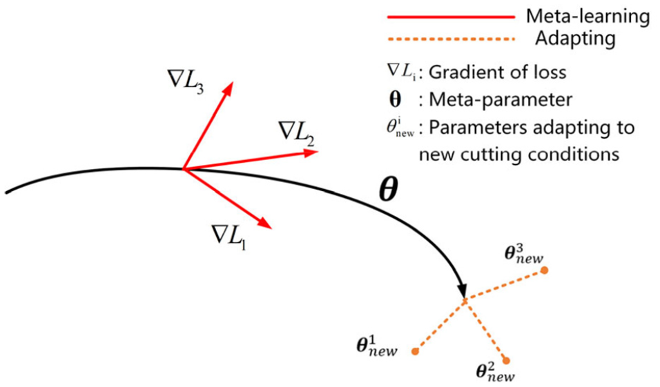
The meta-learning mechanism.

So, the mechanism for learning to learn (meta-learning) is applied to quickly adapt new tasks, after trained by different tasks. The key idea of meta-learning is to train a model’s parameters during a meta-learning phase on a set of tasks such that a few gradient steps, or even one single gradient step, which can produce good results on new tasks. It can be viewed as establishing a general representation broadly adaptable to different tasks.

A base-model in meta-learning is a tool wear prediction model under a specific cutting condition. The architecture of base-model directly impacts the accuracy of tool wear prediction.

Tool wear is a process that changes over time. The current tool wear is related to the previous wear state during a period of time. For this reason, the monitoring signal features of the prior tool wear state will be used for predicting the current tool wear.

RNN is a sequential neural network model in which connections between units form a directed loop. RNN is usually used for data related to sequential tasks. It takes the input sequence as an element from the input layer at a time, maintains a “state vector” in the loop layer, and implicitly contains historical information about all past elements of the sequence. The history information is passed to the current output layer or the next cycle layer. RNN has the powerful ability to capture context information in sequences of different lengths, which is suitable for processing time-series tasks such as tool wear prediction. Tool wear data is auto-correlated and the current tool wear value can be calculated from the current sensor monitoring signals and historical data from the previous time period. In the tool wear prediction model, the order of the data related to the tool wear monitoring signal should be considered, and a model should be constructed using auto-correlation data to describe the dynamic process. Therefore, the tool wear monitoring signal data is “context sensitive” data. Under this circumstance, a class of RNN - Long Short Term Memory (LSTM) is adopted to establish the prediction model by considering the entire tool wear related information. LSTM is a variant of RNN, which is used to solve the gradient vanishing problem of long-sequence RNN model. Using LSTM, the law of tool wear over time can be implicitly learned, and the model parameters can be fine-tuned by collecting labeled samples at the beginning of a new operating condition, which is more suitable for changing conditions, such as corners or arcs, than traditional fully connected neural networks.

As the base-model depicted in Figure 1, LSTM is used to learn abstract representation of input features with time sequence, and then output of LSTM is used as the input of fully connected layers to predict the current tool wear. Therefore, the structure of prediction module consists of LSTM units, and four layers in each prediction process: one feature input layer, the recurrent layer, the hidden layer and the fully connected regression layer. Firstly, the features $Fe a_{i}$ extracted and selected from several continuous segments of time are combined as the input layer $FEA$ . In the LSTM structure, the hidden layer of the first LSTM is taken as the input layer of the second LSTM, and the second hidden layer is passed through the last fully connected regression layer to export the result, as shown in formula (5) and (6):

h = LST M ({Fea}_{1}, {Fea}_{2}, \dots, {Fea}_{s})

(5)

P_{s + 1} = f_{3} (f_{2} (H_{2} \cdot h_{k}^{2} + b_{2}) + b_{3})

(6)

Where $LSTM$ is the LSTM operator; $h$ is the hidden states of the LSTM; $H_{2}$ , $b_{2}$ , and $b_{3}$ are the weights and bias of hidden layer and regression layer. $f_{2}$ and $f_{3}$ are activation functions, $P_{s + 1}$ is the tool wear output of prediction module. One base-model is trained under one specific cutting condition. All the parameters of the base-model i can be expressed as the base-parameter $θ_{i}^{'}$ .

The parameters of the overall structure of the model are studied, including the stacking depth of the neural network model, the number of neurons in each layer, and the selection of the activation function. The control variable method is used to quantitatively analyze the impact of different parameters on the overall performance of the base-model. The optimal value of each parameter is selected for the final tool wear prediction model.

The final structure and hyperparameter of the base-model are as follow: the input layer including 20 units, one hidden layer including 20 units, time steps of LSTM is set as 4, the output layer including one unit as the tool wear value.

Case study

In this paper, 13 sets of experiments are designed, of which nine sets are used for the training of the meta-learning model, and nine sets are used to test the tool wear prediction accuracy of the continual learning under changing cutting conditions. Reasonable selection of cutting parameters for machining titanium alloy can ensure that the cutting tool is in continuous wear state. The flank wear of each cutting tool ranged from 0.10 mm to 0.40 mm for each experiment.

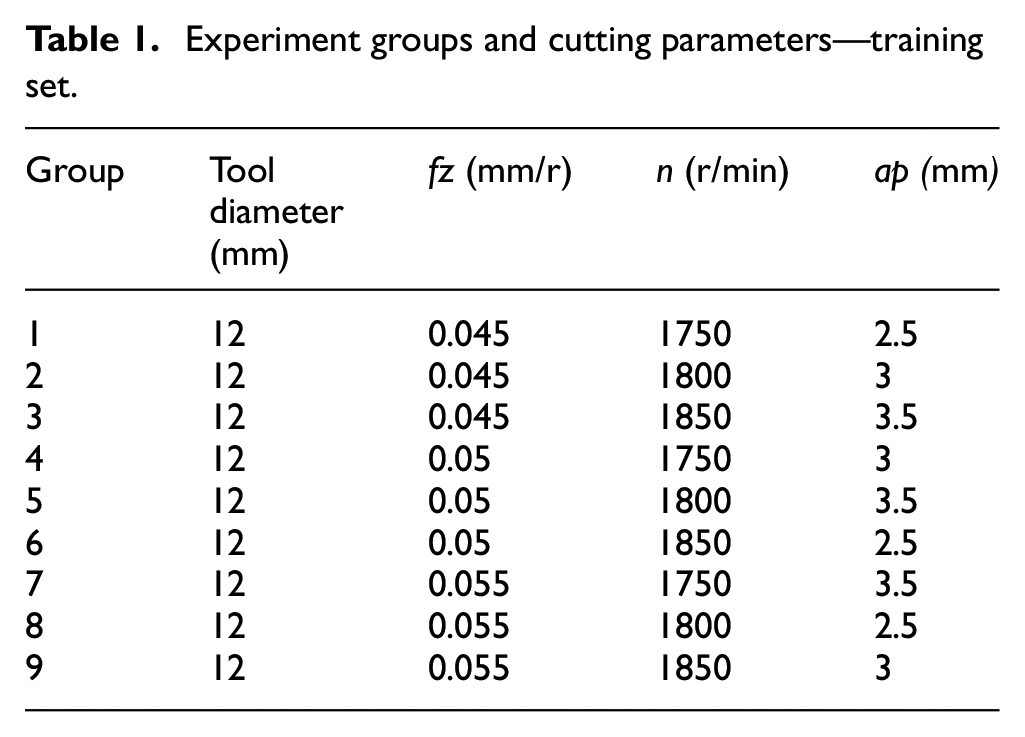
In the experiments for obtaining training samples, the cutting tools used were carbide end milling tools with parameters of 12*12*24*90*R1, the cutting parameters change in the range of: spindle speed (n: 1750 r/min–1850 r/min), feed per tooth (fz: 0.045 mm/r–0.055 mm/r), and cutting depth (ap: 2.5 mm–3.5 mm), as shown in Table 1.

Table 1.

Experiment groups and cutting parameters—training set.

Group	Tool diameter(mm)	fz (mm/r)	n (r/min)	ap (mm)
1	12	0.045	1750	2.5
2	12	0.045	1800	3
3	12	0.045	1850	3.5
4	12	0.05	1750	3
5	12	0.05	1800	3.5
6	12	0.05	1850	2.5
7	12	0.055	1750	3.5
8	12	0.055	1800	2.5
9	12	0.055	1850	3

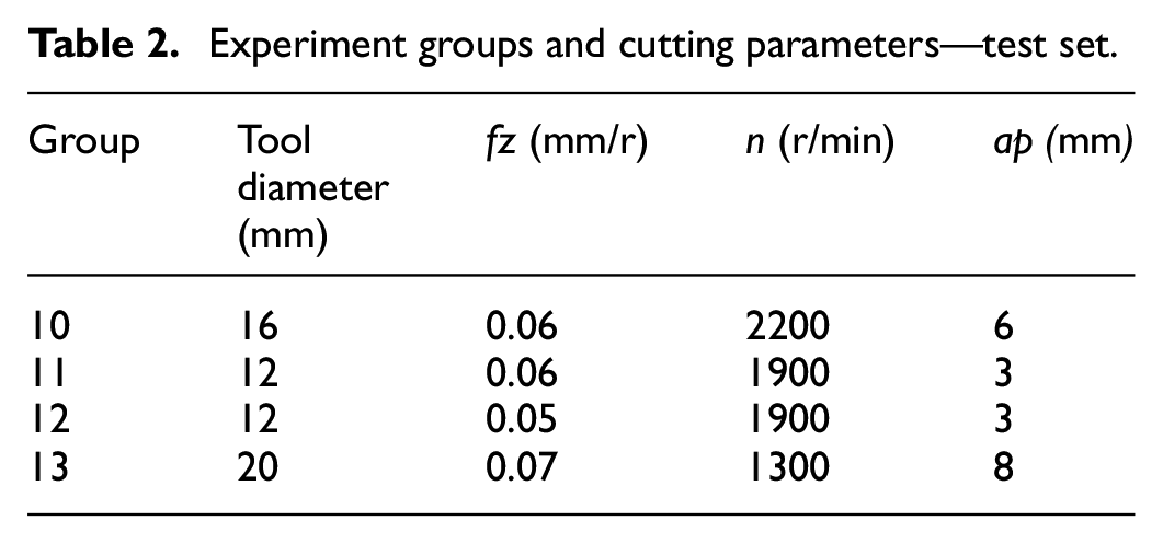
In the experiments for model test, the cutting tools with the same materials are used, with change of tool diameters, D16 and D20 are used, the cutting parameters change in the range of: spindle speed (n: 1300 r/min−2200 r/min), feed per tooth (fz: 0.05 mm/r–0.07 mm/r), and cutting depth (ap: 3 mm–8 mm). It can be found that the cutting tool parameter and cutting parameters are changing dramatically compared with training sets, especially for the last training set, as shown in Table 2. Compared with our previous research,²² the cutting conditions in the test sets change much larger.

Table 2.

Experiment groups and cutting parameters—test set.

Group	Tooldiameter(mm)	fz (mm/r)	n (r/min)	ap (mm)
10	16	0.06	2200	6
11	12	0.06	1900	3
12	12	0.05	1900	3
13	20	0.07	1300	8

As shown in Figure 4, the experiment was performed on a DMG80P machine tool. The part material used in the experiment was titanium alloy TC4, the machining feature is pocket bottom. The vibration, spindle power and current signals were collected during the whole machining process. The vibration sensor is KSI-108M500, and the acquisition frequency is 500 Hz. The spindle power and current signals are collected by the OPCUA of the Siemens CNC system, and the collection frequency is 100 Hz.

Figure 4.

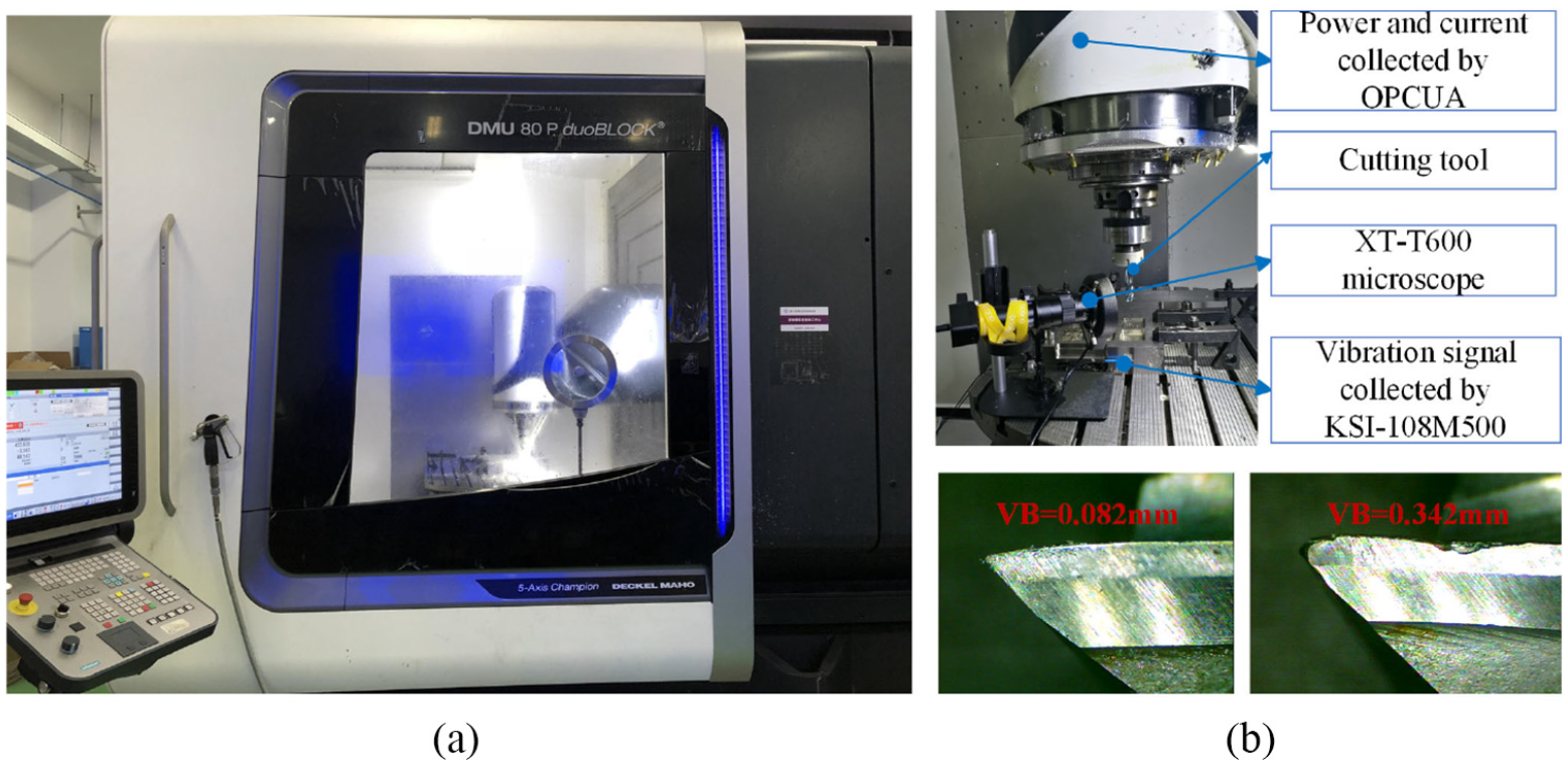
The experiment scene and equipment: (a) experiment scene and (b) experiment equipment.

The tool wear label is collected by an XK-T600 V™ microscope (measurement accuracy is calibrated as: 0.01 mm). In this paper, 246 tool wear labels were actually measured, and about 20 labels were collected under each cutting condition. It should be noted that since the change of the value between two adjacent collected labels is very little, no further intensive collection is required. For each tool, because the collection time between two adjacent labels is short and the tool wear change small, the tool wear can be considered as a gradual change process. In order to further increase the number of labeled samples to help model training, Hermite interpolation method was used to interpolate between two adjacent labels. The number of labeled training samples finally obtained is 4500, which can be better used for training the meta-LSTM model. The number of testing samples in each test set is about 250. During the training process of the meta-learning model, the hyperparameter α is set to 0.001, and the Adam algorithm³¹ is used for optimization. The convergence curve of the training process is shown in Figure 5. The X-axis represents the training epoch and the Y-axis represents the training loss. It can be found that the training process was converged at 100 epoch and the training loss tend to minimum at 700 epoch. During the continual learning process, the hyperparameter $γ$ is set to 1.

Figure 5.

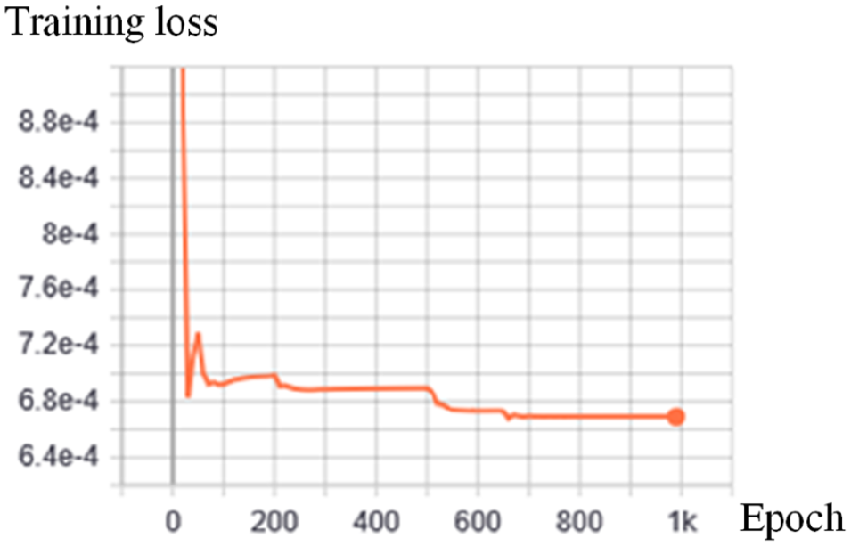
The convergence curve of the training process.

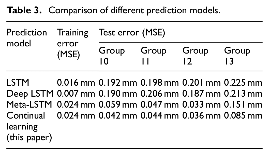
In order to obtain an effective learning model, a large number of debugging experiments have been carried out in the input space dimension, network structure selection, and the number of base-models, etc. Compared with the LSTM model, deep LSTM model and meta-LSTM model, the proposed method improves the tool wear prediction accuracy in different cutting conditions. Specifically in the group 13, in which the task distribution of the cutting condition is much more different from others, the proposed method has greater adaptation than other methods. Table 3 shows the comparison results of different prediction models.

Table 3.

Comparison of different prediction models.

Predictionmodel	Trainingerror(MSE)	Test error (MSE)
Predictionmodel	Trainingerror(MSE)	Group10	Group11	Group12	Group13
LSTM	0.016 mm	0.192 mm	0.198 mm	0.201 mm	0.225 mm
Deep LSTM	0.007 mm	0.190 mm	0.206 mm	0.187 mm	0.213 mm
Meta-LSTM	0.024 mm	0.059 mm	0.047 mm	0.033 mm	0.151 mm
Continuallearning(this paper)	0.024 mm	0.042 mm	0.044 mm	0.036 mm	0.085 mm

Conclusion

This paper proposed a novel method for accurately predicting cutting tool wear in different cutting conditions based on continual learning. A meta-LSTM model is trained for specific cutting conditions and can be easily fine-tuned with very small number of samples to adapt to the new cutting condition. Specifically, the meta-model could be continuously updated during the machining process by learning different tasks sequentially. The meta-parameters are fine-tuned by orthogonal weights modification method with small samples in new cutting conditions.

The experiment results show that the method proposed in this paper can realize the real-time accurate prediction of tool wear under different cutting conditions, and the final prediction error of tool wear is controlled within 0.045 mm. Even in the situation that cutting condition changes largely, the prediction error is 0.085 mm, much smaller than other methods. Compared with existing meta-learning method, the range of adapted cutting conditions could be expanded as the task distribution of new cutting conditions is continuously learned by the prediction model.

The signals collecting method and tool wear labels measurement method are very feasible in industrial circumstance, and smaller labelled samples are required for new cutting conditions, the industrial applicability of the proposed method in this paper will be very good. In the future work, the continual learning model should be further studied for different cutting tool material and different part material.

Footnotes

Declaration of conflicting interests

The author(s) declared no potential conflicts of interest with respect to the research, authorship, and/or publication of this article.

Funding

The author(s) disclosed receipt of the following financial support for the research, authorship, and/or publication of this article: The reported research was funded by National Science Fund of China for Distinguished Young Scholars (grant No. 51925505), National Natural Science Foundation of China (grant No. 51775278, grant No. 51921003).

ORCID iD

Yingguang Li

References

Qin

. Process data analytics in the era of big data. AIChE J 2014; 60(9): 3092–3100.

Snr

DED

. Sensor signals for tool-wear monitoring in metal cutting operations—a review of methods. Int J Mach Tools Manuf 2000; 40(8): 1073–1098.

Zhu

Zhang

Ding

. Tool wear characteristics in machining of nickel-based superalloys. Int J Mach Tools Manuf 2013; 64: 60–77.

Tnshoff

Wulfsberg

Kals

, et al. Developments and trends in monitoring and control of machining processes. CIRP Ann Manuf Technol 1988; 37(2): 611–622.

Finn

Abbeel

Levine

. Model-agnostic meta-learning for fast adaptation of deep networks. In: Proceedings of the 34th International Conference on Machine Learning (ICML), Sydney, NSW, Australia, 6–11 August 2017, ArXiv:1703.03400.

Joudivand Sarand

Shabgard

Jodari Saghaie

, et al. Tool wear estimating model considering modeling improvement factors in electrical discharge machining process based on physical properties of tool electrodes. Proc IMechE, Part B: J Engineering Manufacture 2017; 231(5): 850–866.

Luo

Cheng

Holt

, et al. Modelling flan wear of carbide tool insert in metal cutting. Wear 2005; 259(7): 1235–1240.

Harmouche

Delpha

Diallo

. Incipient fault amplitude estimation using KL divergence with a probabilistic approach. Signal Process 2016; 120(1): 1–7.

Kannan

Padmanabhan

. Analysis of the tool condition monitoring system using fuzzy logic and signal processing. Circuits Syst 2016; 7(9): 2689–2701.

10.

Rech

Giovenco

Courbon

, et al. Toward a new tribological approach to predict cutting tool wear. CIRP Ann Manuf Technol 2018; 67(1): 65–68.

11.

Kuntoğlu

Aslan

Pimenov

, et al. Modeling of cutting parameters and tool geometry for multi-criteria optimization of surface roughness and vibration via response surface methodology in turning of AISI 5140 steel. Materials 2020; 13(19): 4242.

12.

Yang

Zheng

. Investigation on the stress field of milling titanium alloys with micro-textured ball-end milling cutter. Proc IMechE, Part B: J Engineering Manufacture 2019; 233(11): 2160–2172.

13.

Wang

Xie

Zhang

. Tool condition monitoring system based on support vector machine and differential evolution optimization. Proc IMechE, Part B: J Engineering Manufacture 2017; 231(5): 805–813.

14.

Dutta

Pal

Sen

. Progressive tool condition monitoring of end milling from machined surface images. Proc IMechE, Part B: J Engineering Manufacture 2018; 232(2): 251–266.

15.

Imani

Rahmani Henzaki

Hamzeloo

, et al. Modeling and optimizing of cutting force and surface roughness in milling process of Inconel 738 using hybrid ANN and GA. Proc IMechE, Part B: J Engineering Manufacture 2020; 234(5): 920–932.

16.

Badiger

Desai

Ramesh

, et al. Cutting forces, surface roughness and tool wear quality assessment using ANN and PSO approach during machining of MDN431 with TiN/AlN-coated cutting tool. Arab J Sci Eng 2019; 44(9): 7465–7477.

17.

Cheng

Jiao

Shi

, et al. An intelligent prediction model of the tool wear based on machine learning in turning high strength steel. Proc IMechE, Part B: J Engineering Manufacture 2020; 234(13): 1580–1597.

18.

Yang

Wang

, et al. A novel monitoring method for turning tool wear based on support vector machines. Proc IMechE, Part B: J Engineering Manufacture 2016; 230(8): 1359–1371.

19.

Lecun

Bengio

Hinton

. Deep learning. Nature 2015; 521: 436–444.

20.

Zhao

Yan

Wang

, et al. Learning to monitor machine health with convolutional bi-directional LSTM networks. Sensors 2017; 17(2): 273.

21.

Shi

Panoutsos

Luo

, et al. Using multiple feature spaces-based deep learning for tool condition monitoring in ultra-precision manufacturing. IEEE Trans Ind Electron 2019; 66(5): 3794–3803.

22.

Liu

Hua

, et al. A novel method for accurately monitoring and predicting tool wear under varying cutting conditions based on meta-learning. CIRP Ann Manuf Technol 2019; 68(1): 487–490.

23.

Finn

Levine

. Meta-learning and universality: deep representations and gradient descent can approximate any learning algorithm. In: International Conference for Learning Representations (ICLR), Vancouver, BC, Canada, 30 April–3 May 2018.

24.

Goodfellow

Mirza

Xiao

, et al. An empirical investigation of catastrophic forgetting in gradient-based neural networks. Comput Sci 2013; 84(12): 1387–1391.

25.

Parisi

Kemker

Part

, et al. Continual lifelong learning with neural networks: a review. Neural Netw 2018; 113: 54–71.

26.

Zeng

Chen

Cui

, et al. Continual learning of context-dependent processing in neural networks. Nat Mach Intell 2019; 1(8): 364–372.

27.

Singhal

. Training feed-forward networks with the extended Kalman algorithm. In: International conference on acoustics, speech, and signal processing, Glasgow, UK, 23–26 May 1989, pp.1187–1190. New York, NY: IEEE.

28.

Shah

Palmieri

Datum

. Optimal filtering algorithms for fast learning in feedforward neural networks. Neural Netw 1992; 5: 779–787.

29.

Sussillo

Abbott

. Generating coherent patterns of activity from chaotic neural networks. Neuron 2009; 63: 544–557.

30.

Jaeger

. Overcoming catastrophic interference using conceptor-aided backpropagation. In: International Conference for Learning Representations (ICLR), Vancouver, BC, Canada, 30 April–3 May 2018.

31.

Kingma

. Adam: a method for stochastic optimization. In: International Conference for Learning Representations (ICLR), San Diego, CA, USA, 7–9 May 2015, arXiv:1412.6980.

An accurate cutting tool wear prediction method under different cutting conditions based on continual learning

Abstract

Keywords

Introduction

Related works

Cutting tool wear prediction method based on continual learning

Approach overview

Continual learning for cutting tool wear prediction based on orthogonal weights modification method

Meta-learning modeling

Case study

Conclusion

Footnotes

Declaration of conflicting interests

Funding

ORCID iD

References