A multi-particle abrasive model for investigation of residual stress in belt grinding of titanium alloys

Abstract

The titanium alloy blade is a key part of an aero-engine, but its high surface efficiency and precision machining present technical problems. Belt grinding can effectively prolong the fatigue life of the blade and enhance the service performance of the aero-engine. However, the residual stress of the workpiece after belt grinding directly affects its service performance and life. The traditional single particle abrasive model simulation is limited in exploring the influence of grinding process parameters on surface residual stress. In this study, an ABAQUS simulation model of multi-particle belt grinding is established for titanium alloy material, a finite element (FE) simulation is conducted with different technological parameters, and the results are analysed. The critical belt grinding experiment is conducted on thin-walled titanium alloy parts, and the distribution characteristics of surface residual stress after grinding are studied to understand the influence of grinding parameters on the formation of surface residual stress. Comparing the results of the FE simulation and the grinding experiment, the common law of stress change and the prediction model are obtained. The results show that the multi-particle belt grinding simulation is consistent with the belt grinding experiment in terms of the influence of grinding parameters on residual stress. The simulation can serve as a guide in actual belt grinding to some extent. Directions for improving the multi-particle abrasive simulation model are discussed.

Introduction

Titanium alloy is a typical high-performance material, with excellent mechanical properties, high strength, good corrosion resistance, high heat resistance, and adaptability to extreme working environments. It is commonly used in the manufacture of blades for aero-engines, and can significantly improve the aero-engine service life and performance.^1–3 However, titanium alloy has low rigidity and easily deforms. During machining, the springback of the surface is large, which can produce severe friction and lead to processing defects such as burns.^4,5

To improve service performance and fatigue life, belt grinding is used to finish titanium alloy parts.^6,7 Belt grinding offers “flexible grinding” and “cold grinding,” which are widely used in the precision machining of parts that are difficult to machine, such as titanium alloy blades.^8–10 However, there is little targeted research characterizing residual stress on the belt grinding surface of titanium alloy. There is no perfect characterization mechanism, making it difficult to predict the residual stress on the grinding surface to effectively guide the titanium alloy grinding process. Thus, characterization of surface residual stress in belt grinding of titanium alloy parts is significant for enhancing understanding and enriching surface integrity research.

To explore the distribution characteristics of residual stress on the belt grinding surface, Xiao and Huang ¹¹ suggested that the surface integrity could be improved by belt grinding to form micro-reinforced ribs on the surface of titanium alloy blades; the surface residual stress was studied using the FE analysis method. Zou et al. ¹² measured the residual stress of thin-walled TiAl-based alloy components after belt grinding, and studied the influence of grinding pressure on residual stress. Li et al. ¹³ proposed a new method of regulating residual stress in inductive heating assistance grinding, increasing the temperature distribution uniformity along the depth of the grinding process, thus reducing the formation of tensile stress.

To better guide the grinding process, characterization modeling of surface residual stress is essential. Sun et al. ¹⁴ proposed a residual stress prediction model that comprehensively considered the dynamic characteristics; the results were in good agreement with the experimental results. He et al. ¹⁵ studied the surface residual stress of TC17 titanium alloy, characterizing it based on Bragg’s law, and used an experimental method to determine the effect of the titanium alloy belt grinding parameters. Wang et al. ¹⁶ systematically characterized surface integrity including the surface residual stress of nickel-based high-temperature alloys and proposed an optimization prediction model of grinding parameters. Fergani et al. ¹⁷ proposed prediction models for the residual stress of single pass martensite; the test data from the AA2121-T3 milling process agreed well with the model prediction. Zheng et al. ¹⁸ proposed a model to predict the residual stress distribution after riveting. Combined with the residual stress calculated by the model, the fatigue life was predicted using a multiaxial fatigue criterion.

Since the 1970s, the FE method has been widely used to study residual stress in mechanical processing. Nikam and Jain ¹⁹ predicted the residual stress in a micro plasma transfer arc using the FE method. The simulation results indicated that the tensile residual stress is greatest at the junction of the deposition and the matrix, and smallest at the midpoint of the deposition path. Wang et al. ²⁰ established an FE elastic–plastic contact model considering the hardness gradient and initial residual stress. The initial residual stress distribution was obtained by experimental measurement. Choi et al. ²¹ simulated the residual stress of an AA7085 rectangular steel bar using ABAQUS software, compared the simulated residual stress with the experimental results of a longitudinal cutting method, and verified the model accuracy. Satikbaša ²² predicted the residual stress of a multi-pass girth weld using the FE method. It was found that the prediction results with the Maraging model were similar to the experimental results. To evaluate the effectiveness of the FE model in matching the cutting force of ball-end milling, Aydin and Köklü ²³ established an FE model of milling force based on the shear stress, friction coefficient, and chip thickness ratio provided by the orthogonal cutting process, and determined the orthogonal cutting data from the cutting amount of the material parameters. A two-dimensional FE model of the orthogonal cutting process was established by applying the ductile failure criterion based on displacement. ²⁴ The FE analysis method and the effect of deposition stress were used to evaluate the influence of cutting speed on the interface behavior of diamond-coated tools during the cutting of AA356-T6 aluminium alloy. ²⁵

These studies demonstrate that FE simulations can effectively predict the surface residual stress distribution in the grinding process. However, most current FE simulations of belt grinding use single-particle grinding simulation methods to study the belt-grinding mechanism; a multi-particle belt grinding model to represent the actual belt grinding process more completely and predict the impact of grinding parameters on residual stress has not yet been established. Thus, this study presents a simulation model for multi-particle grinding, and analyses the relationship between the residual stress and titanium alloy grinding parameters through an orthogonal simulation. The experimental results are compared with the simulation results to verify the feasibility of the model, identifying surface integrity factors influencing the blade abrasive and their characteristic parameters, and providing theoretical support for the modeling of residual stress on the grinding surface in the belt grinding of aviation titanium alloy blades.

FE simulation of multi-particle belt grinding equipment

Establishment of physical model workpiece

Due to its elasticity, the belt is a small plane contacting the workpiece; its relative speed is fast. Thus, a plane multi-particle belt grinding model can be constructed. Due to the belt elasticity in the actual grinding process, the belt is set as the elastic body. Considering that the hardness of wear particles is greater than that of the workpiece, wear particles can be defined as rigid bodies. The physical model of the multi-particle abrasive simulation for belt grinding is shown in Figure 1. The size of the workpiece is 450  $\mu m$ (length) × 380  $\mu m$ (width) × 150  $\mu m$ (height). The diameter of the grinding wheel is 1250  $\mu m$ , and the width of the grinding wheel is 380  $\mu m$ .

Figure 1.

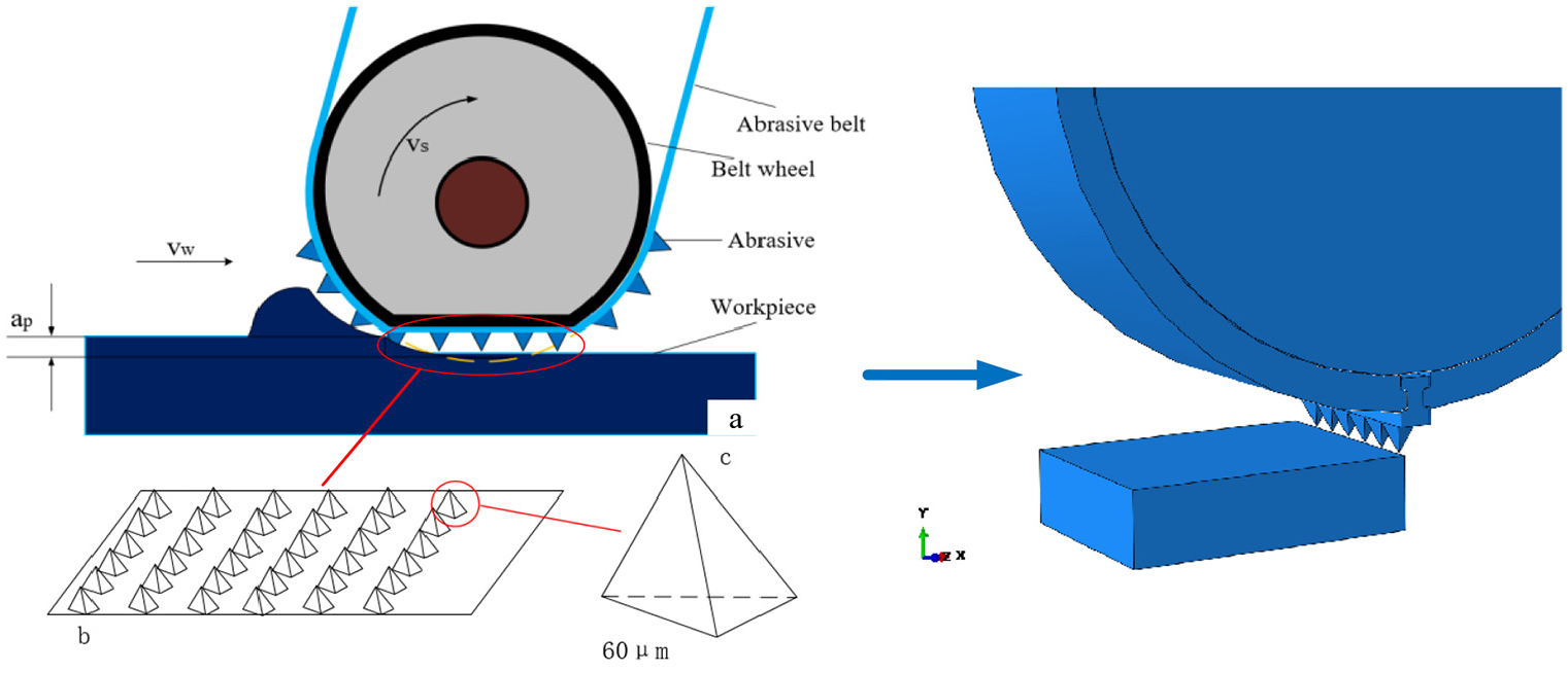
Physical model of multi-particle abrasive grinding.

In Figure 1, $v_s$ is the linear speed, $v_w$ is the feed speed, and $a_p$ is the grinding depth; the abrasive particles on the belt are set as a regular tetrahedron with a side length of 60  $\mu m$ .

Design of FE simulation scheme

In the simulation, we simplified the contact between the belt and the workpiece into a single row of multi-abrasive grinding. The belt is wound on the surface of the grinding wheel. To keep the grinding wheel from rotating, only the belt is set to drive the abrasive grains. The belt and the grinding wheel have a common horizontal feed speed to grind the workpiece. To facilitate calculation, the abrasive particles can be simplified into tetrahedrons in the ABAQUS FE simulation. The processing of the belt to the workpiece can be regarded as the grinding effect of each single abrasive particle on the workpiece. The material properties of the titanium alloy TC4 workpiece are listed in Table 1. The chemical composition of TC4 at room temperature is shown in Table 6.

Table 1.

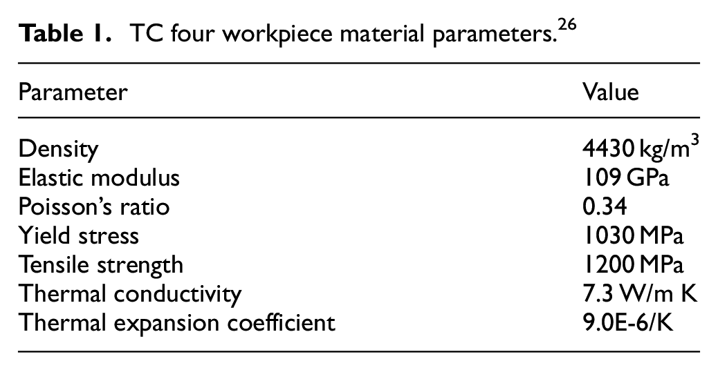
TC four workpiece material parameters. ²⁶

Parameter	Value
Density	4430 kg/m3
Elastic modulus	109 GPa
Poisson’s ratio	0.34
Yield stress	1030 MPa
Tensile strength	1200 MPa
Thermal conductivity	7.3 W/m K
Thermal expansion coefficient	9.0E-6/K

Defining material constitutive relations

In the grinding process, elastic–plastic strain is produced by high temperature and large strain rate. Thus, the influence of strain rate and the thermal softening effect on the hardening stress should be considered when selecting the constitutive model; the Johnson–Cook (JC) constitutive model parameters are selected.

$$\sigma ({\epsilon }_p,\epsilon ,T)=[A+B{\epsilon }_p^{\stackrel{·}{n}}]\left[1+C\ln \stackrel{·}{\epsilon }/{\stackrel{·}{\epsilon }}_0\right]\left[1-{\left(\frac{T-T_r}{T_t-T_r}\right)}^m\right]$$

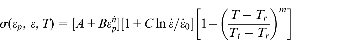
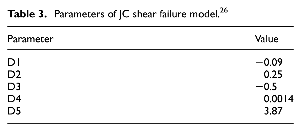
where σ is the Mises flow stress; A, B, C, n, and m are the initial yield stress, strain hardening parameter, strain rate hardening parameter, hardening index, and thermal softening index, respectively; T_t and T_r are the melting point temperature of the material and room temperature, respectively. The JC constitutive model parameters for TC4 material are shown in Table 2. JC adiabatic shear failure criterion can solve the separation problem caused by deformation, distortion, and dislocation by setting the failure parameters in the JC formula. The JC shear failure model parameters for TC4 material are shown in Table 3. The five fracture constants (D1–D5) represent initial failure strain, exponential factor, triaxiality factor, strain rate factor, and temperature factor, respectively.

Table 2.

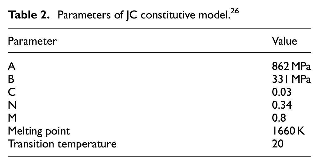
Parameters of JC constitutive model. ²⁶

Parameter	Value
A	862 MPa
B	331 MPa
C	0.03
N	0.34
M	0.8
Melting point	1660 K
Transition temperature	20

Table 3.

Parameters of JC shear failure model. ²⁶

Parameter	Value
D1	−0.09
D2	0.25
D3	−0.5
D4	0.0014
D5	3.87

Analysis and interaction

The dynamic explicit analysis step is used, and the time length is defined as 0.01 s. The interaction attribute is friction-free hard contact and the interaction is general contact. All wear particles are constrained as rigid bodies.

Boundary conditions and loads

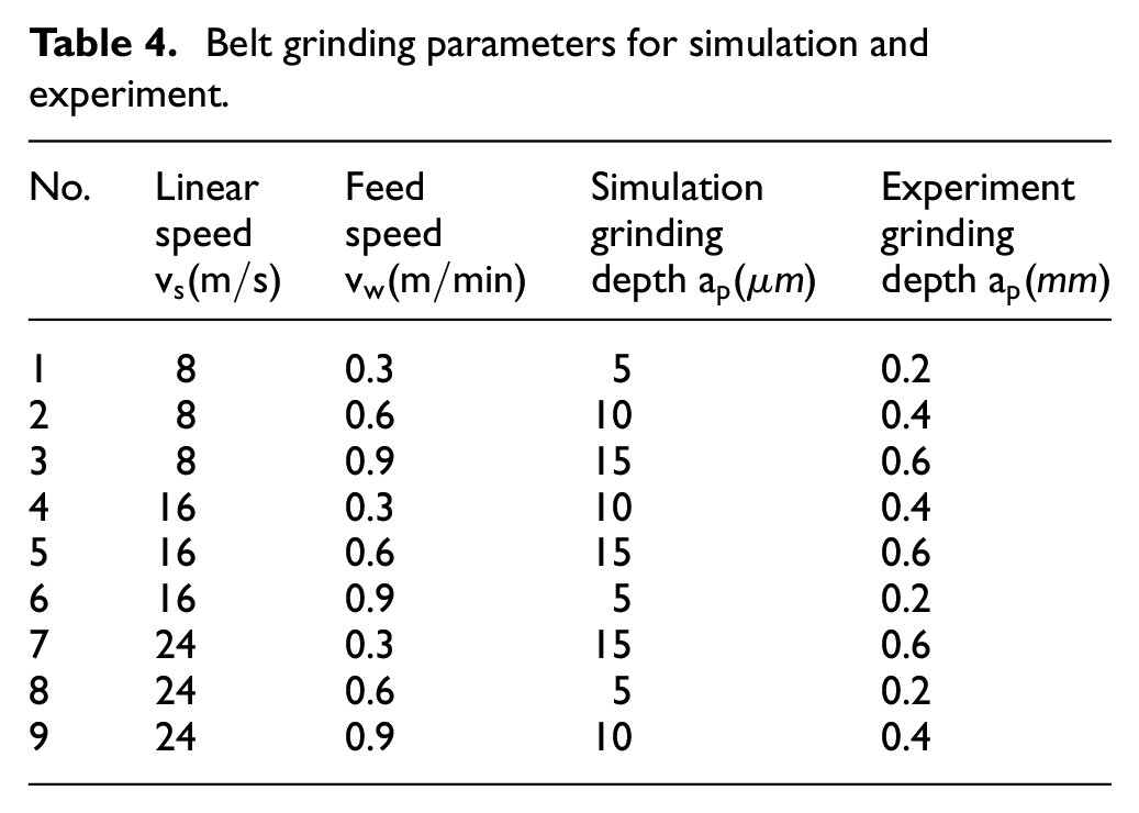
In the simulation, three boundary conditions are applied to the model: the linear speed, grinding depth, and feed speed. An orthogonal experiment with three factors and three levels is used in the simulation design. The simulation parameters for each group are shown in Table 4.

Table 4.

Belt grinding parameters for simulation and experiment.

No.	Linearspeed ${\mathrm{v}}_{\mathrm{s}}(\mathrm{m}/\mathrm{s})$	Feedspeed ${\mathrm{v}}_{\mathrm{w}}(\mathrm{m}/\min )$	Simulationgrindingdepth ${\mathrm{a}}_{\mathrm{p}}(\mu m)$	Experimentgrindingdepth ${\mathrm{a}}_{\mathrm{p}}(\mathrm{mm})$
1	8	0.3	5	0.2
2	8	0.6	10	0.4
3	8	0.9	15	0.6
4	16	0.3	10	0.4
5	16	0.6	15	0.6
6	16	0.9	5	0.2
7	24	0.3	15	0.6
8	24	0.6	5	0.2
9	24	0.9	10	0.4

FE simulation process and result analysis

Simulation process and results

ABAQUS simulation analysis was conducted for the established model; the simulation process is shown in Figure 2.

Figure 2.

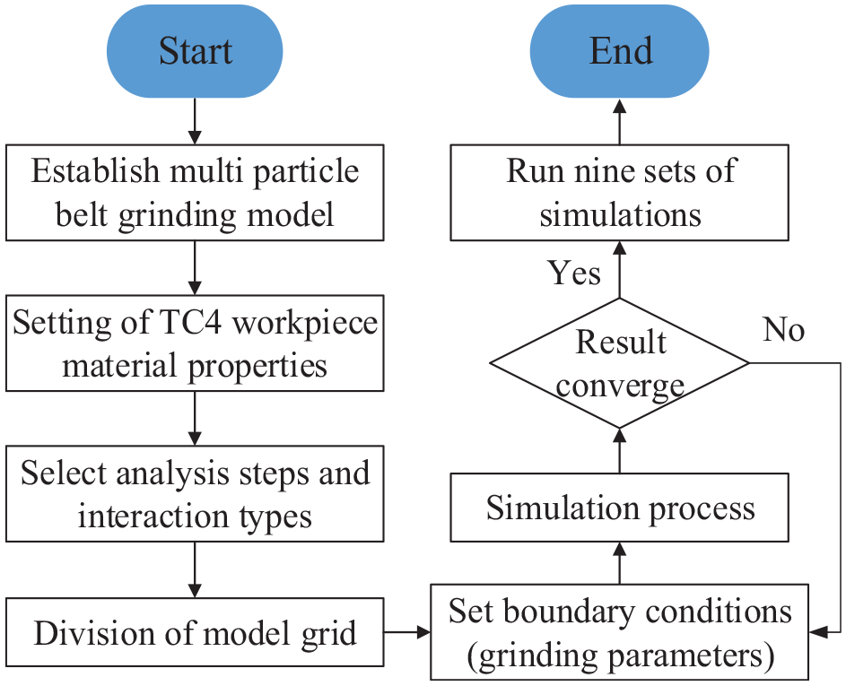
Simulation flow chart.

After repeated grinding of a single row of abrasive particles, a grinding scratch appeared on the surface of the workpiece, as shown in Figure 3. The grindings were gathered on both sides of the scratch under the action of abrasive extrusion and ploughing; a small quantity of grindings reached the edge of the workpiece from the drag of the abrasive particles.

Figure 3.

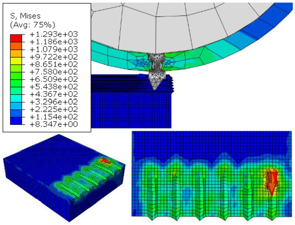
FE simulation of multi-particle belt grinding.

Change of residual stress with time step

With an increase in the simulation time step, the workpiece surface area is expanded, and the surface deformation and accumulation of grindings become more obvious, as shown in Figure 4. Because the linear speed is far greater than the feed speed, the belt produces a repeated grinding effect on the surface of the workpiece. From the stress distribution, it is found that the stress at a given point on the workpiece surface increases with the time step.

Figure 4.

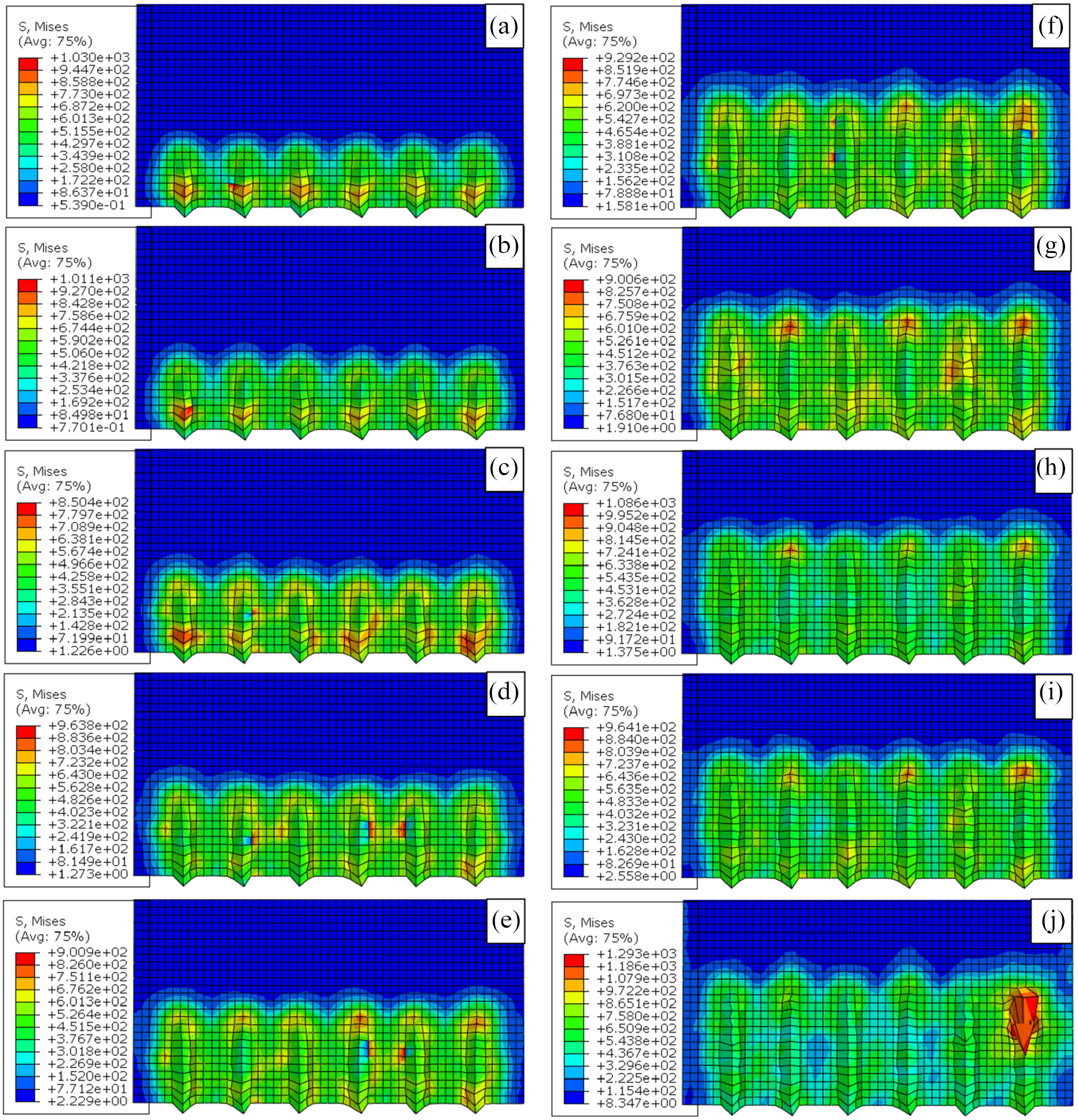
Simulation process changing with time step: (a) 0.005 s, (b) 0.01 s, (c) 0.015 s, (d) 0.02 s, (e) 0.025 s, (f) 0.03 s, (g) 0.035 s, (h) 0.04 s, (i) 0.045 s, and (j) 0.05 s.

To explore whether there is stress accumulation in the elements under the surface of the workpiece during grinding, a unit 48 μm under the surface of the workpiece is considered, and the corresponding stress value in each frame in the simulation process is recorded; the results are shown in Figure 5. After a certain interval, the stress value slightly decreases. The number of falling frames corresponds to the time when the abrasive particles leave the workpiece. At this time, the workpiece is not subject to abrasive grinding and extrusion, and the stress value slightly decreases. However, the overall trend of the curve is increasing, which indicates that the stress under the surface of the workpiece has a tendency to accumulate and increase during belt grinding.

Figure 5.

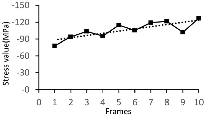
Change in element stress with time step.

Change in residual stress in depth direction for each simulation group

Nine groups of orthogonal simulation were conducted. The simulation stress distribution nephograms are shown in Figure 6.

Figure 6.

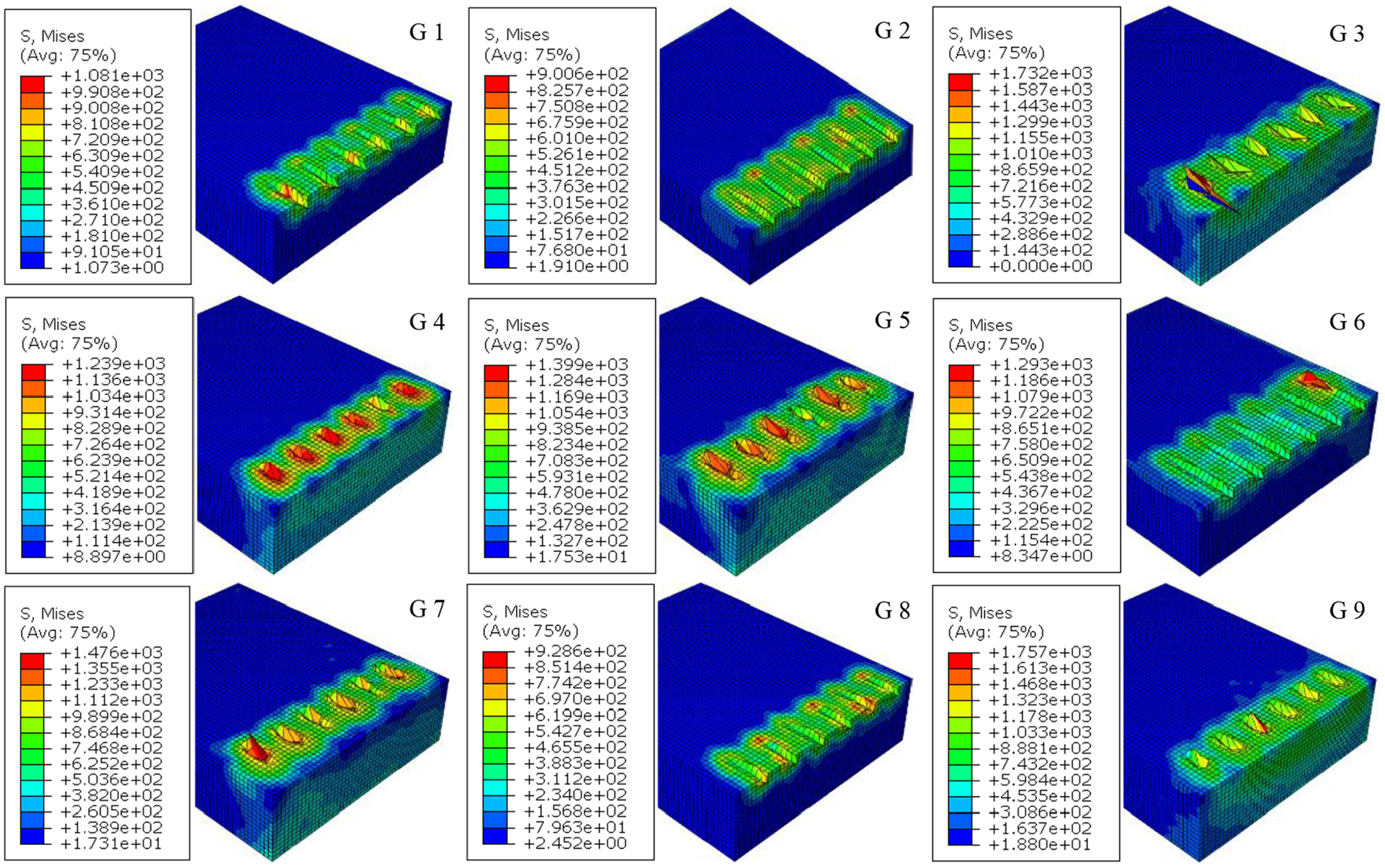
Simulation stress distribution of each group.

In Figure 6, there are obvious scratches in the grinding area directly below the abrasive grains due to the extrusion effect of the abrasive particles; there is also severe deformation and stress. The area near the center exhibits relatively significant grinding deformation due to the compound extrusion of debris from the two sides of the plough. With an increase in grinding depth, the friction between the abrasive particles and the workpiece becomes more severe, leading to a strong adhesion effect between the abrasive particles and the workpiece, with more obvious adhesion. In the simulation of shallow grinding depth, the interaction between abrasive particles and the workpiece is mainly mechanical extrusion; the adhesion is not obvious, and the groove in the processing area is concave.

In Figure 6, the minimum grinding depth in groups 1, 6, and 8 is 5 μm. The surface grinding accumulation height is small and the scratches are clear and uniform. The maximum grinding depth in groups 3, 5, and 7 is 15 μm. Obviously, the grinding accumulation is greater, the deformation is more severe, and the surface stress is high. The grinding deformation in the third group is the most significant. In comparing the simulation parameters, the grinding speed and feed speed in the third group are the greatest. At maximum grinding depth, an increase in the feed speed increases the severity of the surface grinding deformation of the workpiece.

The depth direction unit under the grinding area of the workpiece in each simulation group is shown by the arrow in Figure 7(a). The stress values of 15 elements from top to bottom at corresponding positions in groups 1–9 of the simulation were output and plotted, as shown in Figure 7(b). In the nine simulation groups, the variation in workpiece residual stress with depth shows a downward trend. For example, in group 6, the stress value between the first element and the fifth element decreases from 665.71 to 97.538 MPa. In contrast, from the fifth element to the 15th element, the stress value decreases from 97.538 to 73.6567 MPa. The range of decrease in this section is greatly reduced because a significant stress concentration occurs where the abrasive particles are in contact with the workpiece surface, resulting in a greater change in stress near the surface. As the depth increases, the stress away from the workpiece surface changes little. Similar results were obtained for the other eight simulation groups, indicating that the residual stress decreases rapidly in belt grinding.

Figure 7.

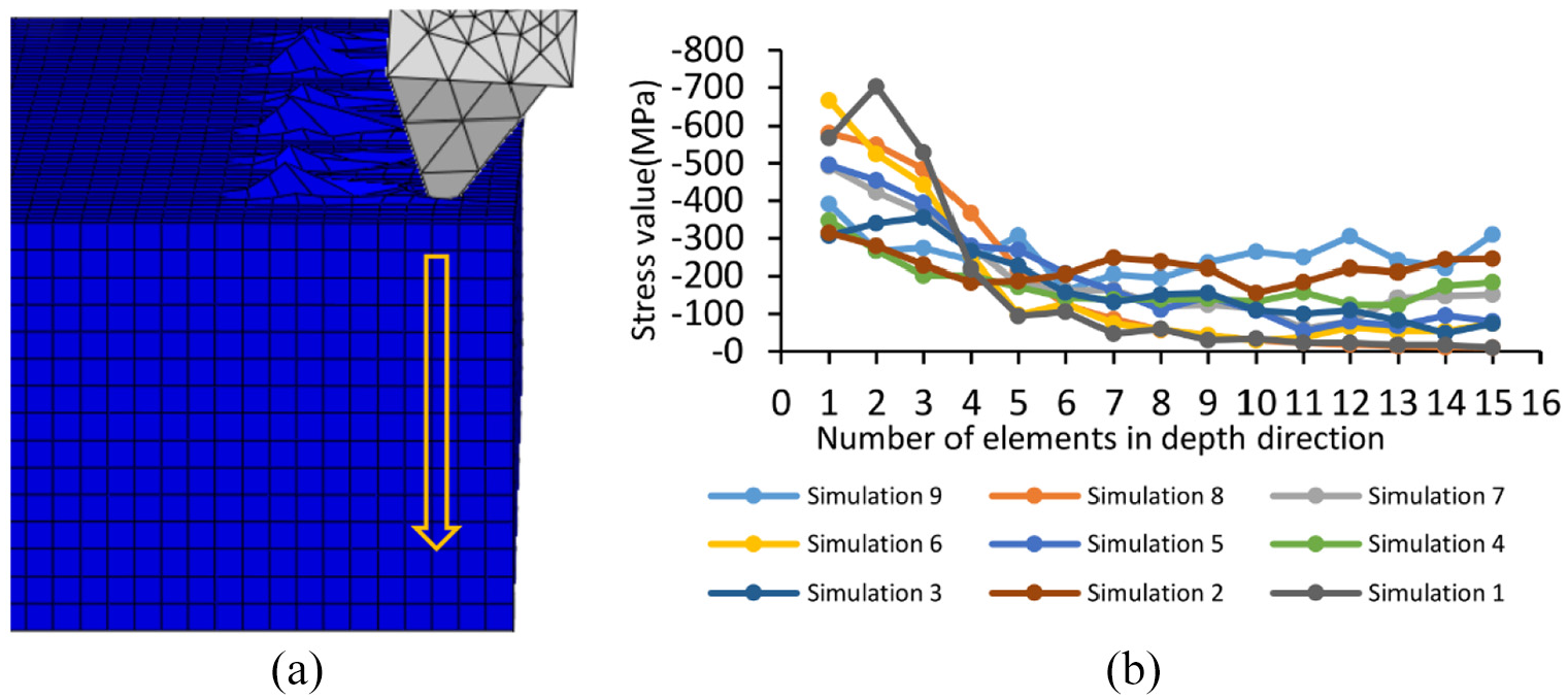
(a) Depth direction unit and (b) stress distribution in depth direction for each simulation group.

Analysis of variation in residual stress with grinding parameters

After the simulation, the stress values of six elements evenly distributed at 20 and 28 μm under the workpiece surface in nine simulation groups were considered; the average value of six stresses represents the residual stress for each group. The simulation result is shown in Figure 8.

Figure 8.

Relationship between residual stress and (a) linear speed, (b) feed speed, and (c) grinding depth.

• (1) Relationship between surface residual stress and linear speed

In Figure 8(a), the residual stress distribution scatter diagram is shown according to the linear speed from low to high, and the change trend line is obtained by linear regression analysis of the scattered points. With an increase in linear speed, the residual stress at two depths decreases.

The residual stress at 28 μm depth is smaller than at 20 μm depth. Because the grinding depth in groups 3, 5, and 7 is the largest, the residual stress of these groups at 20 and 28 μm is the maximum, −470.39, −589.22, −392.21, −290.242, −264.449, −234.988 MPa, respectively.

• (2) Relationship between surface residual stress and feed speed

Similarly, in Figure 8(b), the residual stress distribution scatter diagram is shown according to the feed speed. With an increase in feed speed, the residual stress at two depths increases, and the increase in slope is small. The stress at 20 μm depth is much greater than at 28 μm depth. Due to the uneven distribution of wear particles, a smaller depth produces a more obvious stress concentration near the abrasive particles, resulting in a greater fluctuation in the stress curve at 20 μm depth.

• (3) Relationship between surface residual stress and grinding depth

In Figure 8(c), the residual stress distribution scatter diagram is shown according to the grinding depth. With an increase in grinding depth, the residual stress at two depths increases; the stress curve for 20 μm depth increases more obviously, reflecting that a greater depth produces a less obvious change in stress.

Experimental design of belt grinding for thin-walled titanium alloy parts

Experimental belt grinding method

The critical grinding used in this experiment refers to grinding with a belt that has been passivated but has not reached the degree of blunt grain. In this condition, the plough and the grinding effect are weakened, and the sliding friction effect is greatly increased. A residual stress layer is formed on the surface of the workpiece by rolling, regulating the surface residual stress and improving the fatigue strength of the workpiece.

The critical belt grinding experiment was conducted on thin-walled titanium alloy parts to study the distribution characteristics of surface residual stress after grinding, explore the influence of grinding parameters on the formation of surface residual stress, and guide the subsequent research. The angle between the belt grinding head and the workpiece plane was 60°, using the traditional reciprocating grinding scheme. The specific parameters are shown in Figure 9(a).

Figure 9.

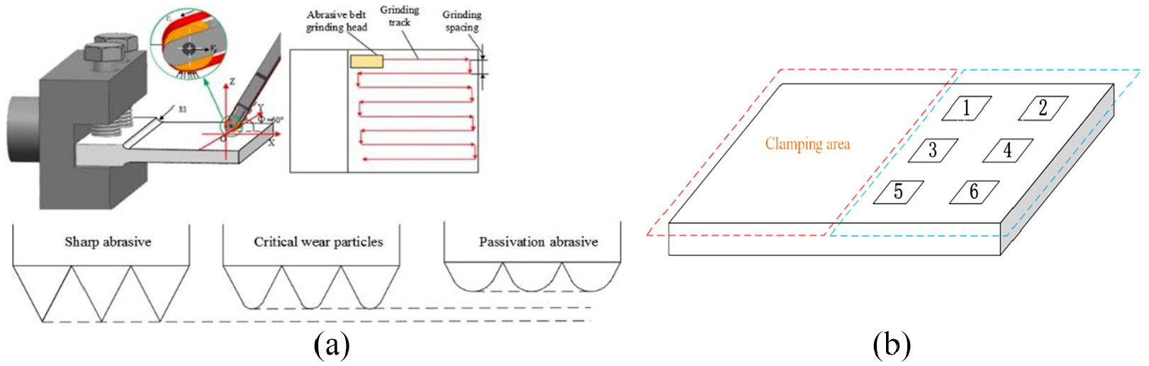
(a) Grinding scheme and (b) distribution of measuring points.

Considering the maximum residual stress at a depth of $1.2\mathrm{\mu }\mathrm{m}$ after belt grinding, ¹⁵ the selected detection depth was $1.2\mathrm{\mu }\mathrm{m}$ . To reduce the influence of random error, six measuring points were selected on the surface of the workpiece; the average of the measured values at these six points was used as the final result. The distribution of measuring points is shown in Figure 9(b).

An orthogonal experiment with three factors and three levels was designed. The factors were linear speed, feed speed, and grinding depth. The grinding parameter settings are shown in Table 4.

Belt linear speed $v_{\mathrm{s}}$ can be obtained from the spindle speed through formula conversion:

$${\mathrm{v}}_{\mathrm{s}}=\frac{\mathrm{D}\mathrm{\pi }\mathrm{n}}{60\times 1000}$$

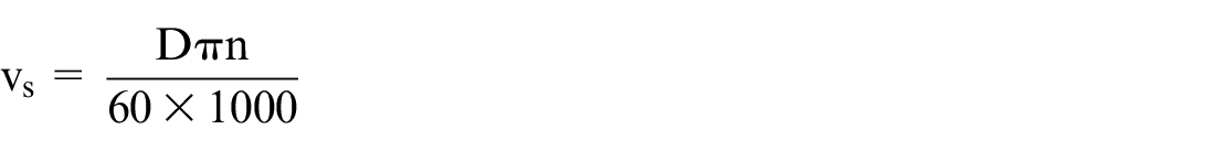
where D is the diameter of the main shaft belt wheel and n is the spindle speed. Grinding depth $a_p$ and feed speed $v_w$ can be controlled by setting the parameters of the NC machine tool during programming.

Experiment setup

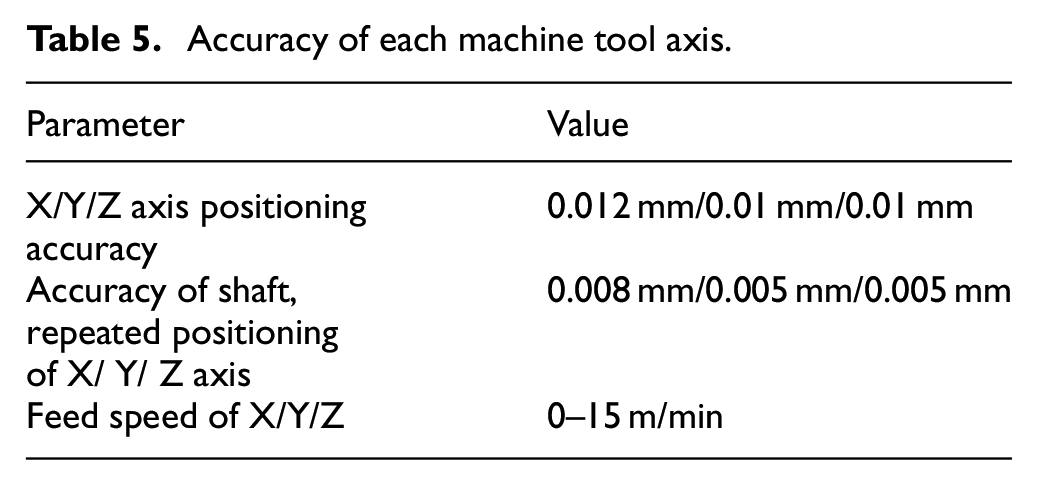
This experiment was conducted on a seven axis–six linkage adaptive CNC belt grinding machine; the equipment is shown in Figure 10(a) and (b). The accuracy of each spindle is shown in Table 5.

Figure 10.

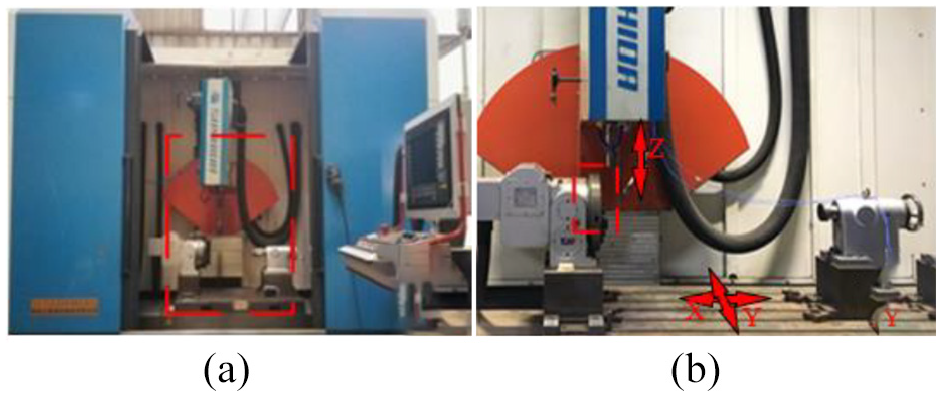
Machine tool structure and test platform: (a) seven axis–six linkage adaptive CNC belt grinding machine and (b) Partial enlarged view.

Table 5.

Accuracy of each machine tool axis.

Parameter	Value
X/Y/Z axis positioningaccuracy	0.012 mm/0.01 mm/0.01 mm
Accuracy of shaft,repeated positioningof X/ Y/ Z axis	0.008 mm/0.005 mm/0.005 mm
Feed speed of X/Y/Z	0–15 m/min

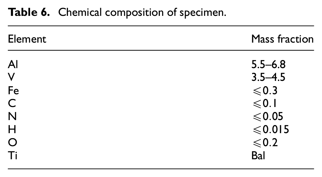
A TC4 (Ti-6Al-4V) titanium alloy plate with dimensions of 170 mm × 100 mm × 2 mm (length × width × thickness) was used in the experiment. The chemical composition at room temperature is shown in Table 6.

Table 6.

Chemical composition of specimen.

Element	Mass fraction
Al	5.5–6.8
V	3.5–4.5
Fe	$\le 0.3$
C	$\le 0.1$
N	$\le 0.05$
H	$\le 0.015$
O	$\le 0.2$
Ti	Bal

A ceramic alumina belt (XK870F) produced by the 3 M company in the United States was used. The particle size was P240#, 2540 mm × 5 mm.

Detection of residual stress

X-ray diffraction is a non-destructive testing method that is widely used for residual stress detection. The basic principle to measure residual stress considers the measured diffraction displacement as the original data, and the measured result as the actual residual strain. The residual stress is calculated from the residual strain using Hooke’s law.

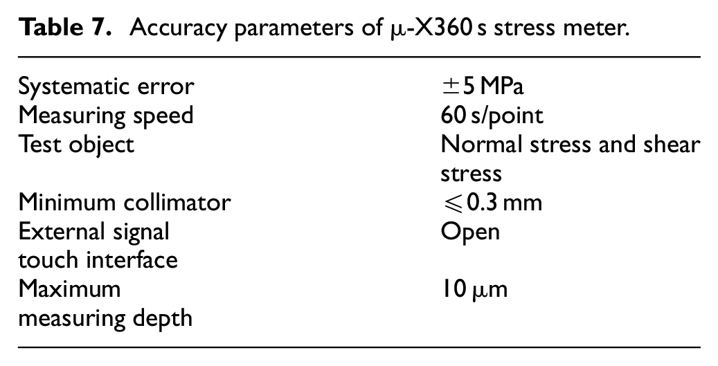
The μ-X360s stress instrument used in this experiment is portable and can conduct non-destructive stress detection on the processed parts. It is based on the full 2-D detection technology and the cos α analysis method. Compared with a traditional 1-D x-ray detector and the sin2Ψ analysis method, the μ-X360 s can obtain all of the Debye diffraction rings in one round of target shooting through a circular two-dimensional detector to calculate residual stress. The μ-X360 s eliminates the need for a precision goniometer for measurement and provides a positioning tolerance of ±5 mm, making field measurements possible. The measurement precision parameters are shown in Table 7.

Table 7.

Accuracy parameters of μ-X360 s stress meter.

Systematic error	±5 MPa
Measuring speed	60 s/point
Test object	Normal stress and shearstress
Minimum collimator	≤0.3 mm
External signaltouch interface	Open
Maximummeasuring depth	10 μm

Mechanism of residual stress on belt grinding surface

Residual stress refers to stress that remains in the body after the external causes of stress are removed. The causes of surface residual stress can be summarized as follows.

• (1) Cold plastic deformation: During grinding, cold plastic deformation occurs on the workpiece surface as a result of the grinding force.

• (2) Hot plastic deformation: In the grinding process, grinding heat leads to thermal expansion of the surface layer of the workpiece. The temperature of the inner layer is lower, which results in thermal plastic deformation, producing compressive stress in the surface layer and the inner layer.

• (3) Residual stress caused by the change in metallographic structure: Different metallographic structures have different densities. Changes in the surface microstructure produce changes in volume. When the volume expansion of the surface layer is restricted by the matrix, compressive stress is generated; otherwise, tensile stress is generated.

The stress of the surface layer after grinding represents the interaction of these three factors. They may act unequally, which comprehensively affects the distribution of the surface prestress. The residual stress on the workpiece surface is equal to the sum of the residual stresses caused by each factor.

$$\mathrm{\sigma }={\sigma }_{\mathrm{cool}}+{\sigma }_{\mathrm{heat}}+{\sigma }_{\mathrm{Phase}}$$

In the formula,

$\mathrm{\Sigma }$  = Total residual stress

${\sigma }_{\mathrm{cool}}$  = Cold deformation residual stress

${\sigma }_{\mathrm{heat}}$  = Residual stress of thermoplastic deformation

${\sigma }_{\mathrm{Phase}}$  = Transformation residual stress

Comparison of simulation and experiment laws for belt grinding

Results of belt grinding simulation and experiment

The measuring points on the surface of the thin-walled parts after belt grinding were checked using the stress meter; the average of the measured values was used as the final result, as shown in Table 8.

Table 8.

Experiment results.

No.	Residual stress (MPa)
1	−173.73
2	−224.36
3	−263.84
4	−197.88
5	−242.71
6	−194.35
7	−185.51
8	−151.73
9	−193.79

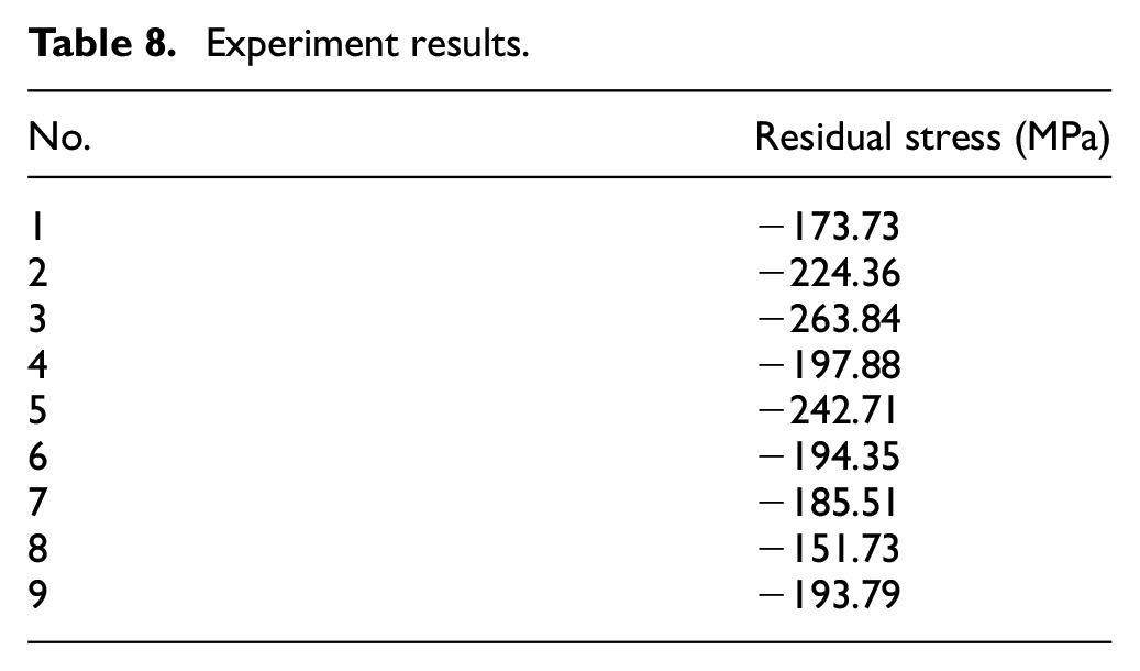
In Table 8, the surface residual stress of the test piece is compressive stress. The residual compressive stress can counteract and relieve the internal stress during the movement and deformation of the workpiece, reducing the actual stress to improve the fatigue life of the workpiece. Thus, the fatigue life of a titanium alloy workpiece is improved after belt grinding. The residual stress on the titanium alloy surface is approximately −200 = MPa. Compared with a grinding wheel, which reaches −2000 = MPa surface residual stress under similar conditions, belt grinding exhibits obvious advantages in controlling the surface residual stress of the specimen.

Figure 11 shows the residual stress error curves at 28 and 20 μm depth in the simulation and experiment. It is observed that the residual stress error at 28 μm depth is much smaller; the maximum error is 21% and the minimum error is 4%.

Figure 11.

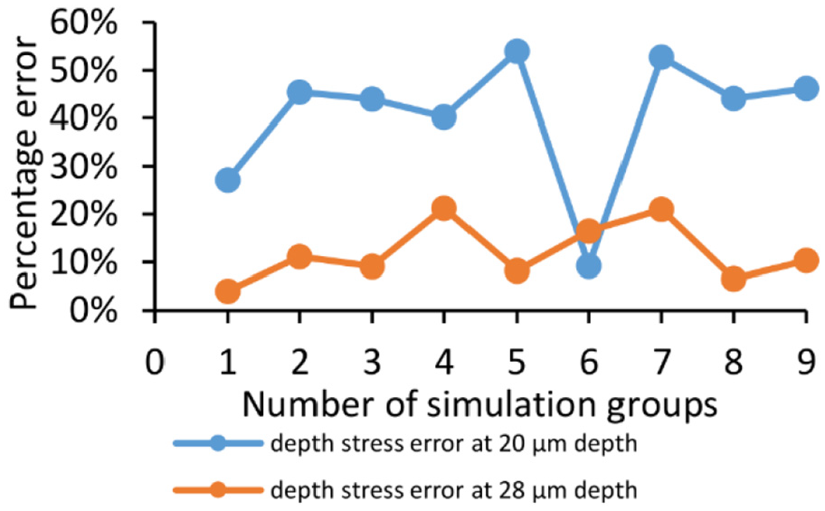
Residual stress error in simulation and experiment.

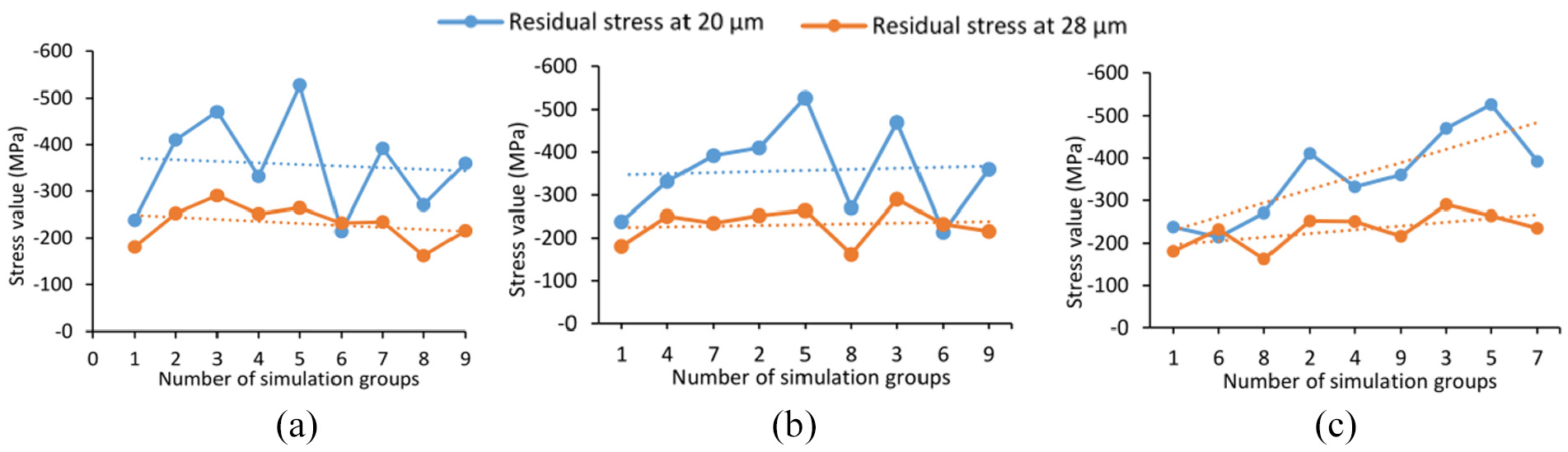
Comparison of relationship between residual stress and linear speed

In Figure 12(a), with an increase in linear speed, the surface residual stress of the test piece gradually decreases. With an increase in linear speed, the number of abrasive grains per unit time increases, and the total heat flow intensity in the grinding area increases, leading to an increase in grinding temperature and generation of greater tensile stress, which counteracts the compressive stress produced by mechanical extrusion between abrasive particles and the surface of the specimen, and reduces the surface residual stress.

Figure 12.

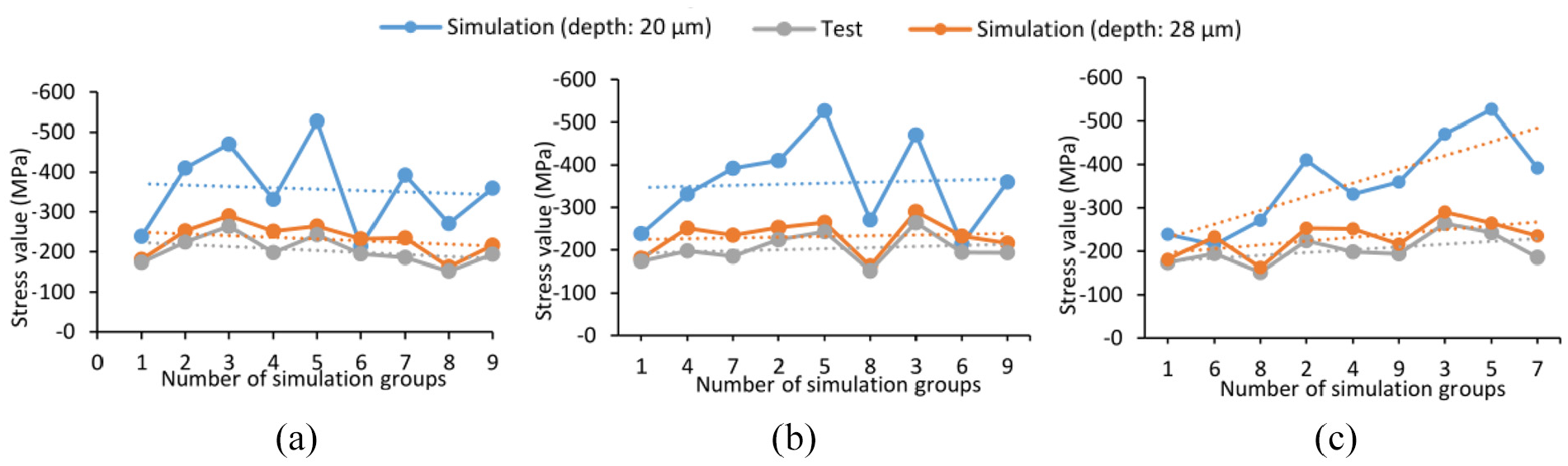
Relationship between residual stress and (a) linear speed, (b) feed speed, and (c) grinding depth.

In Figure 12(a), the linear regression trend lines (dotted lines) of the simulation and experiment are consistent, and the slope is similar. It is observed that a larger grinding depth produces greater residual stress at the same linear speed. For example, in groups 1, 2, and 3 in the simulation, the linear speed of the belt is the same, and the grinding depth for group 3 is the largest (15 μm); the stress at the two depths are −470.39 and −290.242 MPa. The grinding depth for group 1 is the smallest (5 μm), and the stress values are −238.41 and −181.077 MPa. In groups 1, 2, and 3 in the experiment, the linear speed of the belt is the same, and the grinding depth of group 3 is the largest (0.6 mm); the stress value is −263.84 MPa. The grinding depth of group 1 is the smallest (0.2 mm), and the stress value is −173.73 MPa.

The residual stress in the simulation is higher than in the experiment, partly because the simulation model is simplified and the mesh accuracy is not high. Another possible reason is that the elastic modulus of the belt was set too high in the simulation, and the yielding performance during grinding was not as good as in the experiment.

Comparison of relationship between residual stress and feed speed

In Figure 12(b), with an increase in feed speed of the grinding head, the surface residual stress increases. A greater feed speed reduces the contact time of a single abrasive particle, resulting in decreased heat accumulation, decreased tensile stress caused by grinding heat, increased mechanical extrusion, and increased surface residual compressive stress.

In Figure 12(b), the linear regression trend is consistent in the simulation and the experiment, and the slope is similar. In the simulation and experiment, the effect of feed speed on the residual stress is not obvious. The residual stress fluctuation at 20 μm depth is greater in the simulation; the residual stress fluctuation at 28 μm depth is similar in the simulation and the experiment.

Comparison of relationship between residual stress and grinding depth

In Figure 12(c), with an increase in grinding depth, the surface residual stress increases gradually because the grinding force and the grinding temperature increase. However, due to the characteristics of “cold grinding,” the grinding temperature does not increase much. Thus, the tensile stress caused by grinding temperature is less than the compressive stress produced by mechanical extrusion. This phenomenon is more obvious at greater grinding depths.

In Figure 12(c), the linear regression trend lines (dotted lines) for the simulation and experiment are consistent; the slope is larger in the simulation than in the experiment. In the simulation, with an increase in grinding depth, the residual stress of the workpiece at 20 μm depth increases from −214.22 to −589.22 MPa. The increase is more rapid in the simulation because the belt grinding yield is better in the actual test, reducing the grinding force to some extent and producing slow residual stress growth. In the simulation, when the depth is small, the belt has poor yielding ability, and less heat and tensile stress are caused by high temperature, causing the residual stress to increase more rapidly. When the depth is large, the residual stress increases slowly because the stress concentration is not obvious.

Conclusion

1. A numerical model of multi-particle abrasive grinding was established and an orthogonal simulation was conducted. Through experimental verification, it was found that linear speed and residual stress exhibit a negative correlation; feed speed and residual stress exhibit a positive correlation; grinding depth and residual stress exhibit a positive correlation.

2. The multi-abrasive belt grinding simulation is consistent with the actual belt grinding experiment in terms of the influence of grinding parameters on residual stress, verifying the multi-abrasive simulation prediction model for belt grinding, which can serve as a guide for actual belt grinding to some extent.

3. The sizes of the simulation model and experimental model are different. It was found that the stress in the simulation model was different at different depths. A depth with a residual stress similar to the experimental value can be used to predict the residual stress in belt grinding. Compared with the experimental error, the stress at 28 μm depth is much smaller than at 20 μm depth, and fits the experimental stress curve better. Thus, the simulation results at 28 μm depth better simulate the actual belt grinding experiment.

4. The simulation results show that the residual stress under the workpiece surface accumulates and increases with the repeated extrusion of abrasive particles. After the simulation, the residual stress on the workpiece surface decreases with increasing depth; the residual stress decreases faster closer to the workpiece surface.