
Abstract
Layered fracture frequently occurs in the deforming process of QStE700 medium-thickness steel plates under tensile loading. In this study, the morphology of a layered fracture was observed via scanning electron microscopy, and the mechanism of the layered fracture was also analyzed. Based on the three-dimensional digital image correlation technique, a section analysis method was adopted for determining the true stress–strain curve including the necking process. A modified Bridgeman’s equation was adopted to transform the true stress–strain curve into the equivalent stress–strain curve. At the time of layered fracture occurrence, the equivalent strain and stress triaxiality of differently shaped specimens were obtained and fitted to a linear exponential relationship equation. The equation was the layered fracture criterion function and combined with the finite element method (FEM) simulations for determining the damage criterion of the layered fracture of a certain specimen. The FEM-simulated equivalent strain was consistent with the experimental equivalent strain of the layered fracture. Summarizing, the proposed method to predict the layered fracture of a QStE700 medium-thickness steel plate is effective and can be adopted in the study and control of layered fracture.
Instruction
QStE700 medium-thickness steel plates having high strength and ductility have been extensively used in automobile girders and other parts. In small-radius forming or roll bending processes, layered fracture occurs with the increase in the stress in the thickness direction. Around a layered fracture area, the strength extension clearly decreases and easily causes broken failure and shortens the part lifetime. The phenomenon of the layered fracture of a QStE700 medium-thickness steel plate cannot be disregarded, and theoretical research and practical applications should be developed.
Some studies on layered fracture have been conducted. Yang et al. 1 considered high dislocation density as the main factor for layered fracture, with occluded materials and initial defects serving as crack initiation points. McClintock 2 and Rice and Tracey 3 proved that the plastic fracture of a metal mainly depends on the stress state. Bao and Wierzbicki 4 and Bai and Wierzbicki 5 conducted a series of experiments and simulations, and deduced the relationships between the equivalent strain and the three-dimensional stress. However, the proposed formula could not cover fractures under high stress triaxiality ratios. Park et al. 6 established the limit criteria for forming a fracture, which were proved to be suitable for the prediction of advanced high-strength steel fracture in sheet forming. Yan and Zhao 7 proposed fracture criteria considering ductility loss, and the experimental results were found to be consistent with the predictions. Zhu and Engelhardt 8 established a modified fracture model considering stress triaxiality and shear stress ratio, and the theoretical model was found to be suitable for predicting ductile fracture at both low and high triaxiality. Li et al. 9 proposed a ductile fracture model, which was verified by comparing with the isotropic Mohr–Coulomb (M–C) fracture model. Brünig et al. 10 studied the stress–strain effect on the fracture mode of an aluminum alloy, and established an anisotropic fracture model for ductile metals. Seifi and Hosseini 11 studied crack growth in copper under cyclic loading, and the simulated results were consistent with the experimental ones. Bjurenstedt et al. 12 conducted a tensile test to evaluate the role of Fe-rich intermetallics on the crack initiation in Al–Si alloys. It was concluded that a large α-Fe intermetallic cracks first and subsequently the clusters of α-Fe act as the crack initiations sites. Guo et al. 13 found that the cleavage crack of ductile metal substrates was the result of brittle coating and its fracture. The detrimental effect becomes increasingly clear with the increase in the coating thickness. Bonnen and Topper 14 analyzed a unified crack growth model including both shear and tensile cracking. The crack of a specimen was predicted successfully, and the endurance limits of crack-face interference were estimated reasonably. Zhou et al. 15 investigated cleavage fracture control in pearlitic structures via scanning electron microscopy (SEM) and electron backscattered diffraction (EBSD). The results revealed that a cleavage crack largely deflects at block boundaries, instead of at colony boundaries, and that a pearlite block acts as the dominant substructure in the cleavage crack propagation in pearlitic steels. Wang et al. 16 conducted tests to study the fracture mechanism of different regions in a dissimilar welded joint; it was found that the fracture mode was a combination of brittle and ductile fractures. Concurrently, the weld region had a lower resistance to crack initiation and propagation than the base and interfacial regions. Wee and Choi 17 proposed that the layered fracture theory could be an effective tool to model a slow crack growth; however, it requires numerous input parameters. To verify this, simulations of a slow crack growth in high-density polyethylene were conducted, and the effect of each parameter on the crack growth behavior was investigated.
Recently, the digital image correlation (DIC) technique has been applied in the area of displacement and strain measurement. Siddiqui 18 reported conducting two-dimensional full-field displacement measurements for the analysis and inspection of solid propellant grains, and the comparison of the experimental and finite element model results showed good agreement. Almeida et al. 19 developed the three-dimensional (3D)-DIC technique, which can measure anisotropic, volumetric, and heterogeneous strains. Min et al. 20 used the DIC technique to investigate the effect of strain rate on the Portevin–Le Chatelier behavior of twinning-induced plasticity steel. The results were proved to be more accurate than those obtained by other methods. Ding et al. 21 determined diffused and localized necking strains by uniaxial tensile tests, and evaluated the effect of strain rate on the necking strains using the 3D-DIC technique. Kashfuddoja and Ramji 22 used the 3D-DIC technique to obtain results under full-field strain variations; the experimental results were found to be in good agreement with the finite element results. Bilotta et al. 23 adopted the DIC technique to assess the properties of a fabric-reinforced cementitious matrix (FRCM) material, and it was proved to be a new and effective method to evaluate microstructures and mechanical properties. Nguyen and Young 24 evaluated and predicted forming limit curves of boron steel 22MnB5 sheet at elevated temperatures, based on the finite element method and experiments, the fracture strain trajectory at high temperature was determined by using the ductile cavity growth model.
This study was conducted to predict the layered fracture of a QStE700 medium-thickness steel plate. The layered fracture morphology was observed via SEM, and the mechanism of layered fracture was explored. The true stress–strain curve was obtained by a section analysis method based on the 3D-DIC technique. A modified Bridgeman’s equation was adopted to transform the true stress–strain curve into the equivalent stress–strain curve. At the time of layered fracture occurrence, the equivalent strain and stress triaxiality of differently shaped specimens were obtained and fitted to a linear exponential relationship equation. This relation was adopted for determining the damage criterion of layered fracture by finite element method (FEM) simulations. This study offers a useful guideline for the research and control of layered fracture of medium-thickness steel plates.
Materials and methods
Test specimens
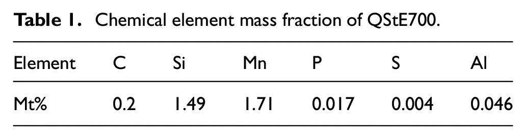
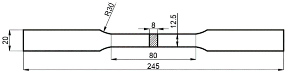
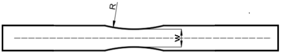
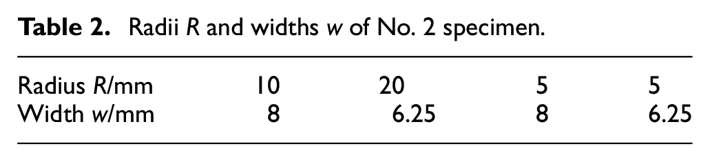
Generally, the thickness of a medium-thickness steel plate is between 4.5 mm and 12 mm. In our research, the experimental object was a hot rolling 8-mm QStE700 steel plate. Its chemical element mass fraction is summarized in Table 1. For the stress–strain curve, the No. 1 specimen, as shown in Figure 1, was designed according to JIS Z 2241:2011; the specimen had a rectangular cross-section. For the study of layered fracture under different initiated stress triaxiality, the No. 2 specimen, as depicted in Figure 2, was designed; its different radii R and widths w are listed in Table 2. The initial triaxiality ratios for the standard (R30w12.5), R10w8, R20w6.25, R5w8, and R5w6.25 tensile specimens were 0.692, 0.788, 0.665, 0.966, and 0.891, respectively.
Chemical element mass fraction of QStE700.
Parameters of No. 1 specimen.
Parameters of No. 2 specimen.
Radii R and widths w of No. 2 specimen.
Testing apparatus
As presented in Figure 3, the DIC measuring system consisted of two 5M-pixel CCD digital cameras (Grasshopper™) and a data acquisition and processing system. 25 Both cameras were used to collect images at 10 fps. The software was Vic-Snap (Correlated Solutions Company). The tensile tests were conducted on a universal testing machine (Reger 300™). The tensile test speed was 3 mm/min.
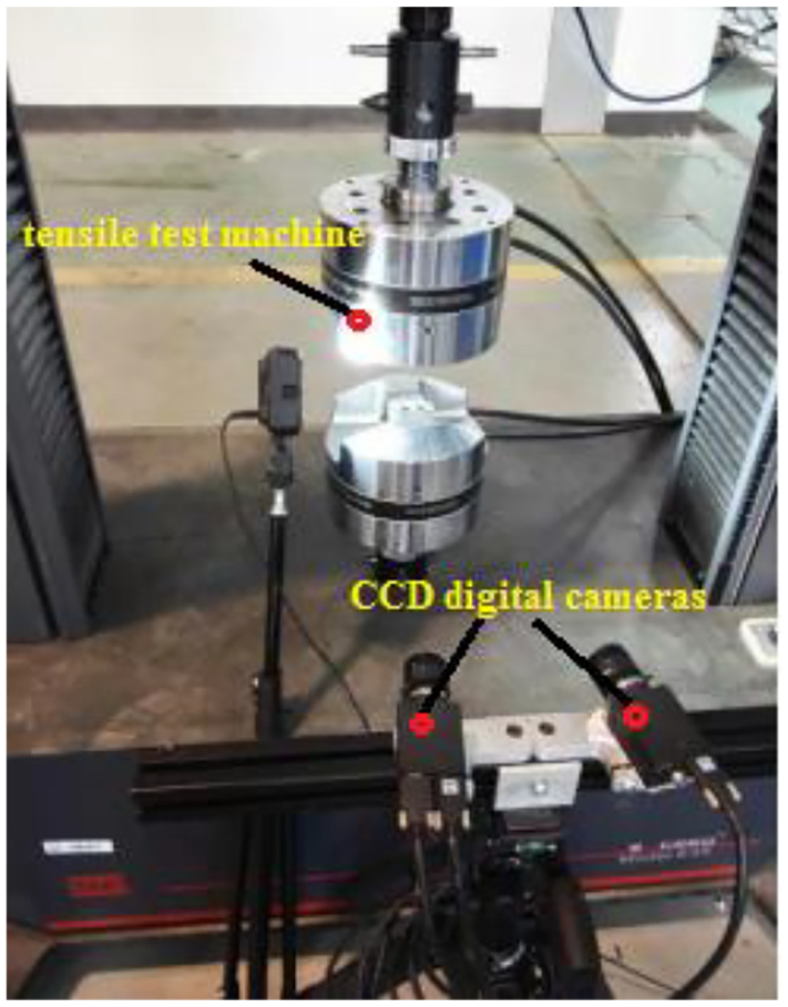
DIC measuring system.
Testing procedure
All the specimens were cut from one steel sheet blank by electrical discharge machining (EDM), and then polished by 80# sandpaper to remove the burrs and oxide layer. The specimen surfaces near the gauge section were decorated with white paint. After 30 min, black speckles were sprayed randomly on the white paint. The decorated specimen was dried at room temperature for 1 h to enhance the adhesion between the paint and the specimen surface.
In the tensile tests, the black speckles were stretched in the longitudinal direction but compressed in the cross direction. Figure 4 shows the strain evolution of the specimen with R30 and w12.5 under tensile loading obtained using the DIC measuring system. Coordinates of the points on the gauge surfaces were obtained by a 3D-DIC post-process. The micro-morphology of the fracture of the specimen was observed via SEM, and chemical elements in the layered fracture surface were detected via energy dispersive spectroscopy (EDS).
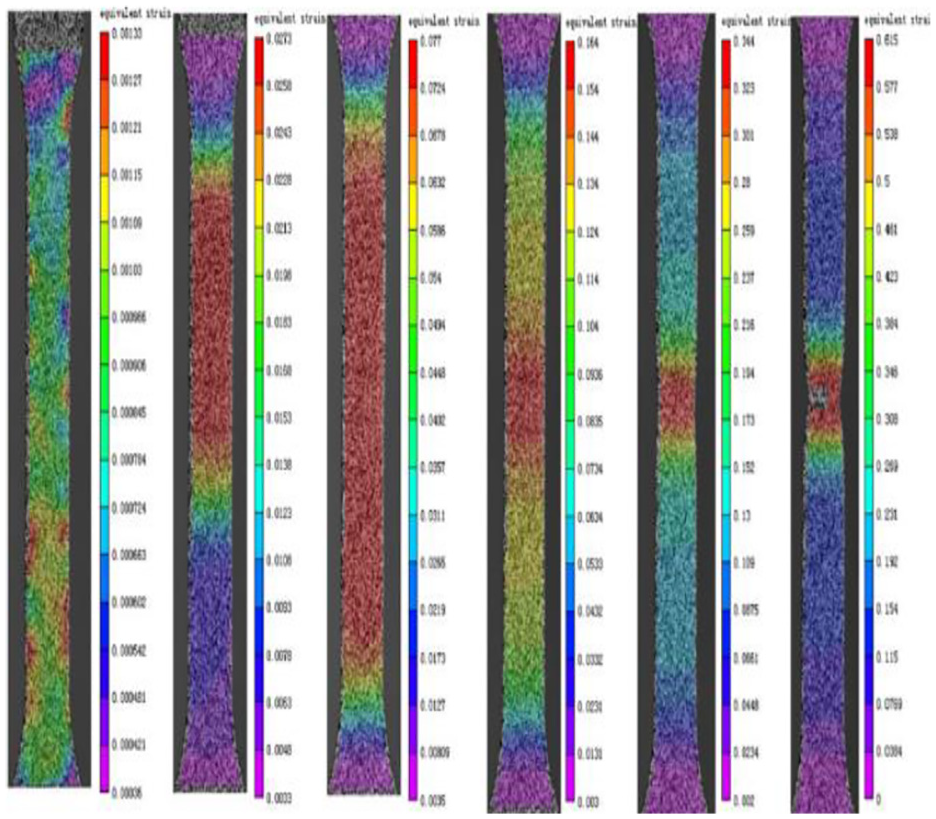
Strain evolution process of standard specimen.
Results and discussions
Layered fracture phenomenon
In the tensile specimen, it is found that layered fracture first occurs in the thickness direction after necking, and tensile fracture occurs after a period of a small tensile deformation. Figure 5(c) displays the engineering stress–strain curve of the specimen shown in Figure 5(a) and (b). It can be seen from Figure 5(c) that an abrupt drop in the engineering stress occurs near the strain of 0.228, which corresponds to the layered fracture of the tensile specimen. The engineering stress–strain curve of the tensile fracture, as presented in in Figure 5(c), shows there is a small amount of deformation and that the stress after the first abrupt drop, again decreases abruptly. After the occurrence of layered fracture, the specimen continues to stretch and deform until it is pulled forward.
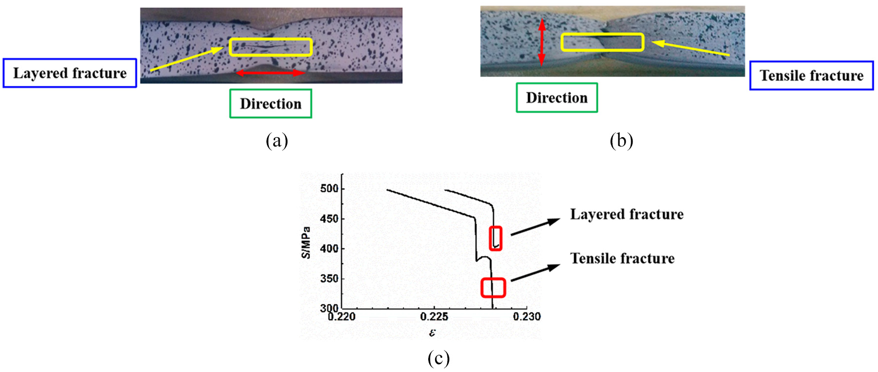
Layered fracture and tensile fracture of medium-thickness steel plate: (a) layered fracture, (b) tensile fracture, and (c) engineering stress -strain curve of medium-thickness steel plate.
The 100× micro-topography of a layered fracture surface is shown in Figure 6(b). Most of the surface area is relatively smooth. The 1000× micro-topography of the layered fracture surface is shown in Figure 6(c). The cross direction “fluvial pattern” and tearing edges were the basic micro-topography. The chemical elements of the layered fracture surface determined via EDS are shown in Figure 6(a). Some broken chips are also found for the mixture of CaS and Al2O3. The layered fracture phenomenon indicates that the broken chips can easily concentrate on the fracture surface and enhance its strength.
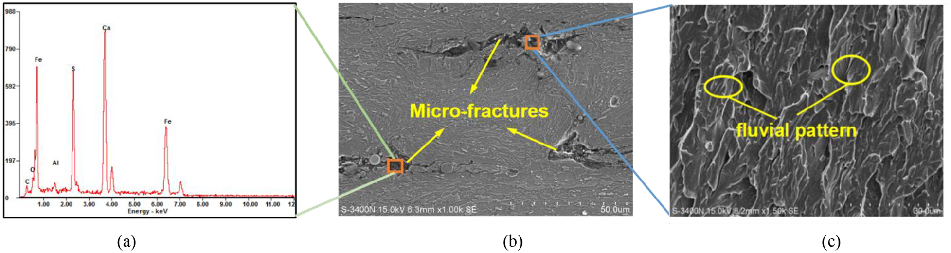
Chemical elements and micro-topography of layered fracture surface: (a) chemical elements, (b) 100× micro-fracture, and (c) 1000× micro-topography.
Layered fracture prediction
Section analysis method based on 3D-DIC test
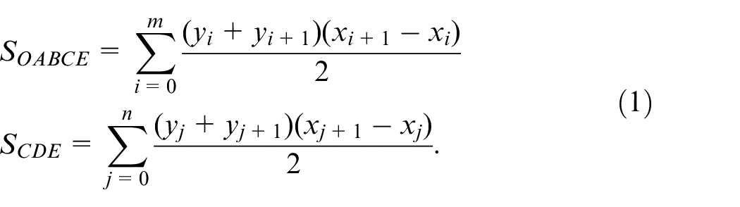
In the tensile test, the cross-section of the specimen was rectangular initially, which changed in the necking process. During the tensile test, the coordinates of the gauge surface points were obtained continuously using the 3D-DIC test system. The thickness mapping of the specimen during the tensile test is shown in Figure 7. The cross-section contours of the necking area were obtained by post-processing. In Figure 8, contour ABCD is one quarter of the cross-section contour of the necking area. Ordinate yB of point B is the maximum, and abscissa xC of point C is the maximum. The contour could be divided into two parts by point C(xC,yC). Point E is the projection of point C onto the X-axis. Area SOABCD is the difference between area SOABCE and area SCDE. Contour ABC was divided into m portions, and the coordinates of the point on the contour are represented as (xi, yi). Similarly, contour CD was divided into n portions, and the coordinates of the point on the contour are assumed as (xj, yj). Areas SOABCD and SCDE were calculated using equation (1), and the one quarter of the cross-section area was calculated using equation (2).

It was assumed that during the tensile process, the cross-section was symmetrical. One total cross-section contour of necking area A was obtained by the quarter contour in Figure 8 and A = 4 × SOABCD. Figure 9 shows the changing process of the cross-section contour in the tensile test. It indicates that the cross-sectional area reduces gradually and the contour shape changes irregularly.
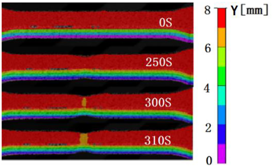
Thickness mapping of specimen.
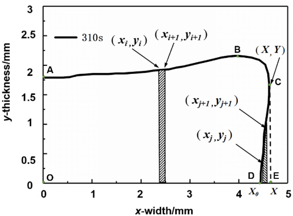
Quarter of cross-section contour.
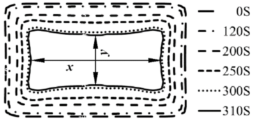
Evolution of specimen cross-section.
The above method is defined as the section analysis method. The method was adopted to calculate instantaneous real section area A of the specimen in the tensile test. Real section area A of the specimen in the necking process is very important for obtaining the stress–strain curve.
Equivalent stress–strain curve
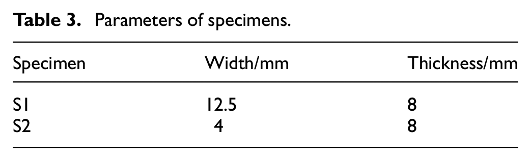
The parameters of two specimens are listed in Table 3. The engineering strain was obtained using a virtual extensometer in the tensile test in Figure 10, and the engineering stress was calculated using equation (3).
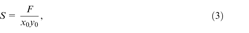
where S is the engineering stress, F is the tensile force,
Parameters of specimens.
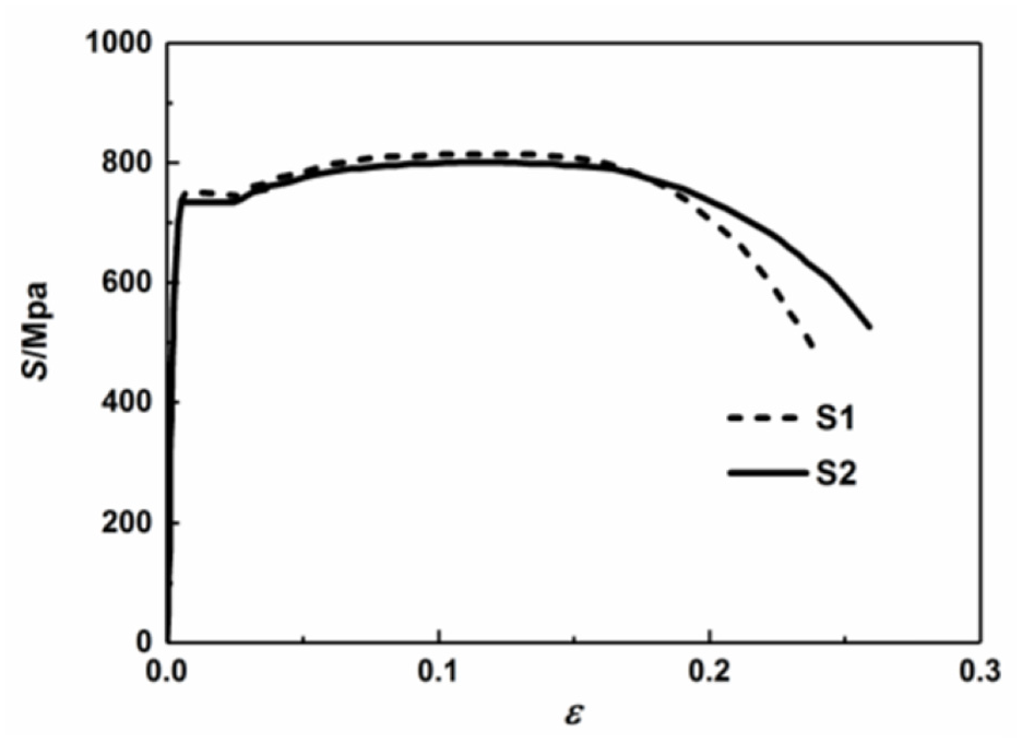
Engineering stress–strain curves of specimens.
The sectional geometry and area during the tensile deformation were obtained, and the true stress–strain curve was derived using equation (4).

where F is the tensile force, A is the instantaneous section area, and
Varied true stress–strain curves are shown in Figure 11. The true stress–strain curves from the 3D-DIC test were almost the same, which suggests that the section area of the specimen had little influence on the true stress–strain curve. All the true stress–strain curves were consistent before the necking. However, in the necking, the true stress–strain curve obtained using the extensometer damps rapidly, whereas that from the 3D-DIC test increases continuously. The traditional tensile test conducted with an extensometer could not yield the true stress–strain curve, including necking, accurately owing to the neglect of the changed section area.
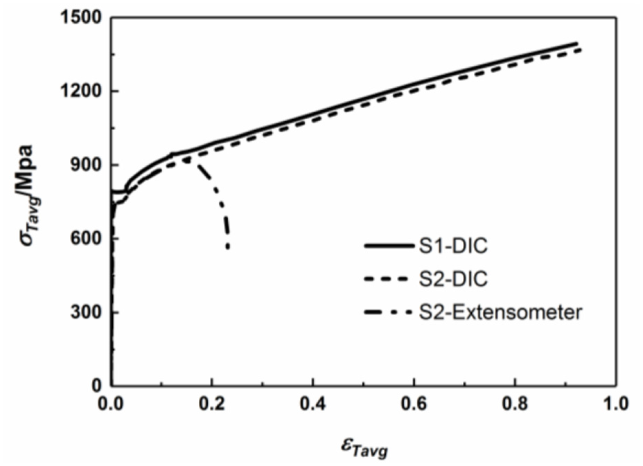
True stress–strain curves obtained using 3D-DIC test and extensometer.
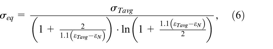
Traditionally, it is widely accepted that material deformation obeys the Hollomoon hardening exponential function relating the yield and the necking stage, as expressed in equation (5). This equation leads to considerable errors in the necking. Therefore, a modified Bridgeman’s equation was adopted to transform the true stress–strain curve into the equivalent one using equation (6).
26
The equivalent strain,

where
where
ABAQUS is a powerful engineering software for performing FEM simulations. Finite element model of the standard specimen was established, which is shown in Figure 13. The mesh type was a C3D8R unit, and the size of each element was 0.5 × 1.0 × 1.0 mm. One end is fixed and the other end is loaded. The tensile displacement is 25 mm and the tensile is uniformly stretched at a constant rate of 3 mm/min. The traditional exponential and modified equivalent stress–strain curves were used as constitutive models for finite element simulation to obtain the true stress–strain curve at different tensile moments.
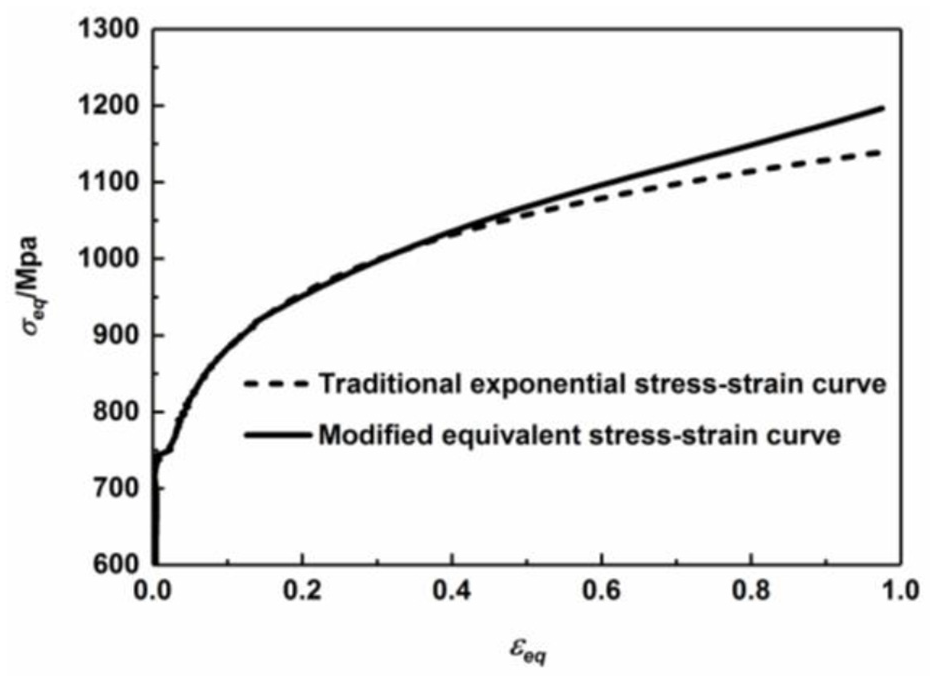
Two types of equivalent stress–strain curves.
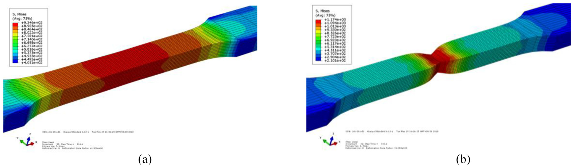
Finite element models for tensile simulation: (a) initial finite element model and (b) necking finite element model.
Figure 14 shows the true stress–strain curves obtained from different methods. The simulated true stress–strain curve based on equation (6) was more consistent with the experimental result. Equation (6) was used for expressing the equivalent stress–strain function including the necking, and adopted in the following FEM simulation of the layered fracture.
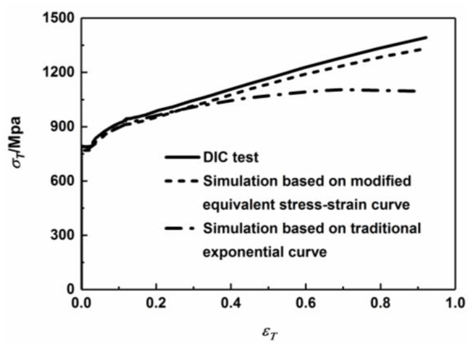
True stress–strain curves from different methods.
Layered fracture criterion function
For differently shaped specimens, at the time of layered fracture occurrence, the stress triaxiality and the equivalent strain were extracted and fitted to a function, which is defined as the layered fracture criterion function.
Finite element models of the differently shaped specimens with different values of R and w were established, which are shown in Figure 18. The mesh type was a C3D8R unit, and the size of each element was 0.5 × 1.0 × 1.0 mm. Based on the layered fracture criterion function, the finite element models without the damage criterion were established, which are displayed in Figure 15.
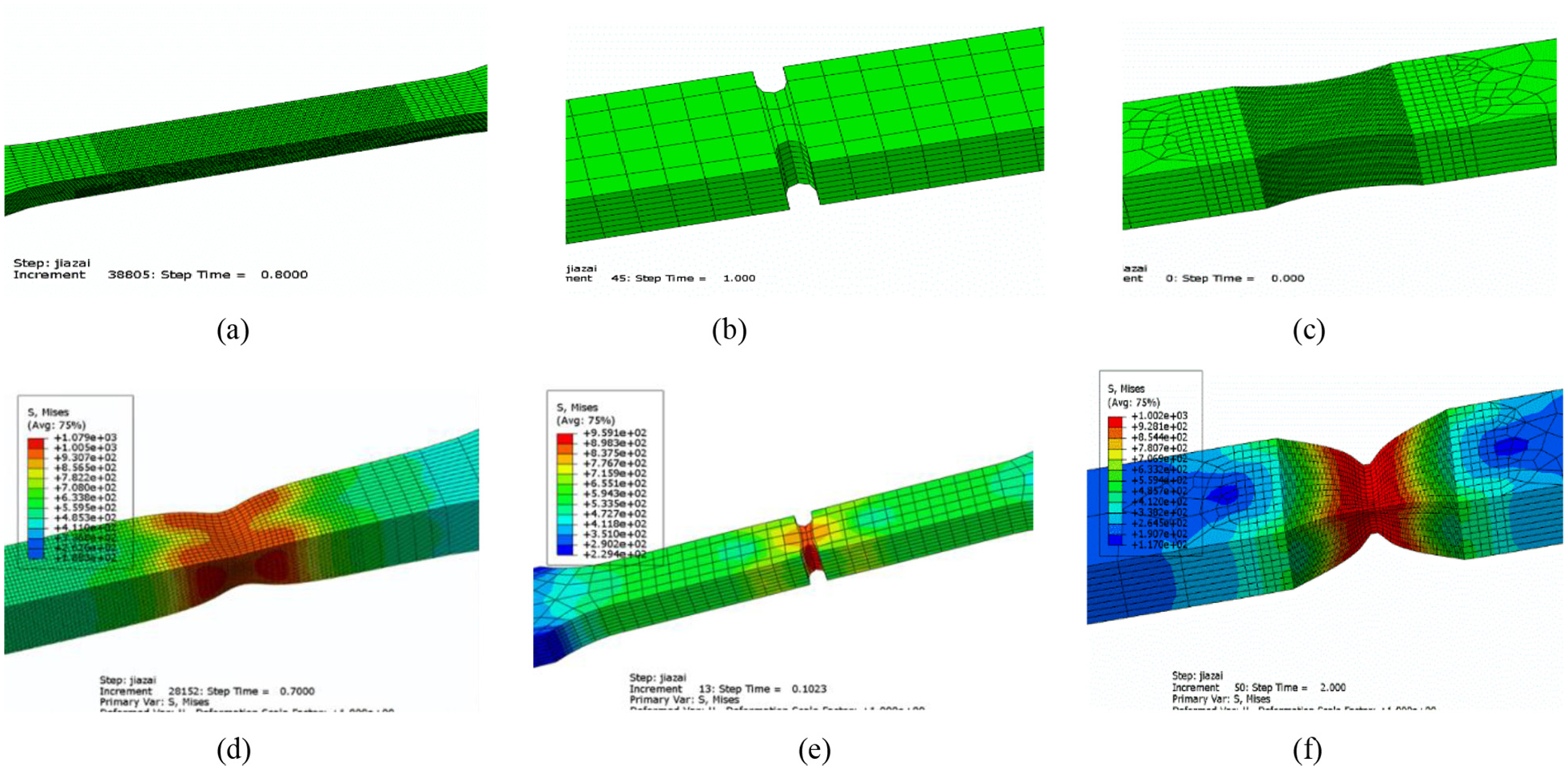
Finite element models of specimens having different shapes: (a) standard specimen, (b) R5w8 specimen, (c) R20w10 specimen, (d) standard specimen, (e) R5w8 specimen, and (f) R20w10 specimen.
In the tensile test, the equivalent strain of the necking area at the time of layered fracture occurrence was obtained by performing a 3D-DIC test. In the tensile FEM simulation, when the strain of the necking area became equal to the equivalent strain in the tensile test, layered fracture occurred, and the equivalent stress triaxiality in the center of the necked area was obtained from the finite element model. The stress triaxiality,
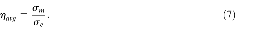
Average main stress,
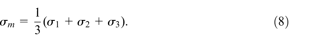
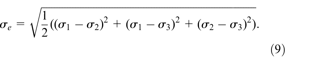
where won-Mises equivalent stress
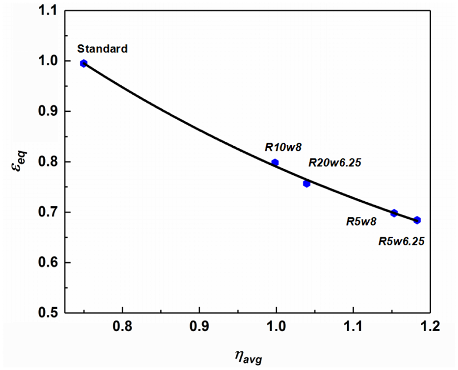
For the differently shaped specimens, the tensile tests and FEM simulations were repeated. At the time of layered fracture occurrence, the relative stress triaxiality and the equivalent strain were obtained and fitted as the layered fracture criterion function, which is shown as a curve in Figure 16. The equation is as follows:

Based on the above research, when the layered fracture occurs, the criterion stress triaxiality and the equivalent strain in the center of the necking area are confirmed to equation (10). For a certain specimen with a particular shape, its stress triaxiality in the layered fracture criterion was determined using equation (10) and FEM simulations. From the FEM tensile simulations, the stress triaxiality and equivalent strain curve was obtained, which is shown in Figure 16. Its intersection point with the layered fracture criterion curve is the layered fracture criterion point, and the coordinates of the point are the stress triaxiality and the equivalent strain of this type of shaped specimen in the layered fracture criterion. Therefore, the stress triaxiality and equivalent strain of the specimens with different shapes in the layered fracture criterion were determined by the layered fracture criterion curve and FEM simulations without the 3D-DIC test.
Layered fracture criterion curve.
The stress triaxiality and equivalent strain in the layered fracture criterion were adopted as the damage criteria in the layered fracture prediction by the FEM. In the FEM simulation, when the equivalent strain reached the critical value, layered fracture occurred.
Application of layered fracture criterion function
For specimen R20w10, the simulated stress triaxiality and equivalent strain curve by the tensile process simulation in ABAQUS was obtained, and is shown as a dotted curve in Figure 17. The coordinate values of the intersection point are the layered fracture criterion stress triaxiality and the equivalent strain, and they are used as the damage criterion in the FEM.
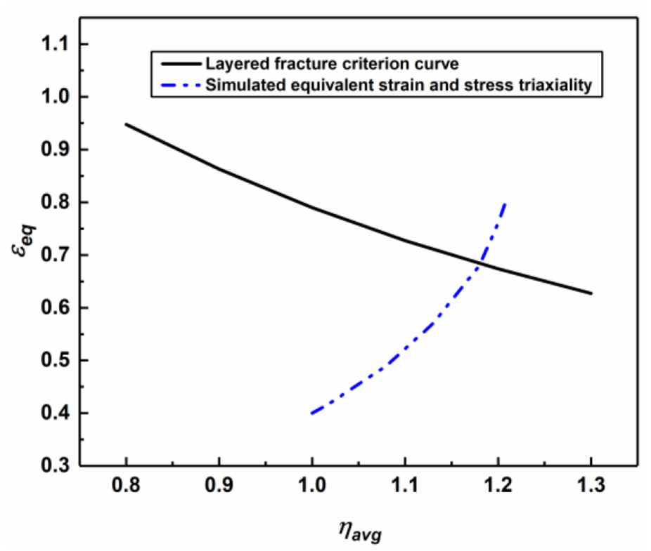
Layered fracture criterion of R20w10 specimen.
As is shown in Figure 18, a finite element model based on the damage criterion was established. The finite element model was simulated by the dynamic analysis module, ABAQUS/EXPICIT. The grid property was changed to display unit grid, and the option of grid deletion was allowed in the calculation. The mesh element type was C3D8R, and the size was 0.5 × 1.0 × 1.0 mm.
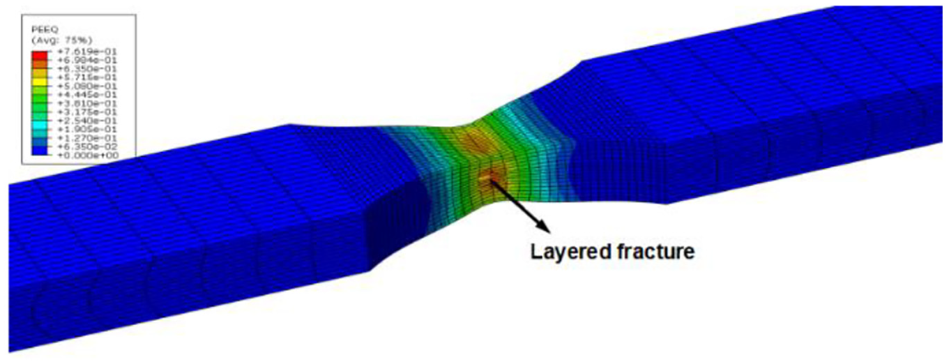
Layered fracture in finite element model.
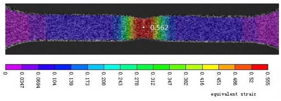
In the 3D-DIC tensile test, specimen R20w10 is shown in Figure 19. From the test and FEM simulation, the equivalent strains at the time of layered fracture occurrence are listed in Table 4. The result showed that the error was 6.42%. Besides, with the same method, the errors were within 5% for specimens R1.25w8 and R5w8 in Table 4.
Tested equivalent strain of layered fracture.
Equivalent strain of layered fracture on main surface.
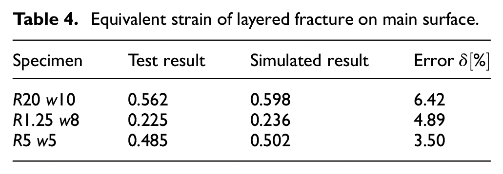
For the tensile tests of different specimens, the stress triaxiality and equivalent strain curve was different; however, at the moment of layered fracture occurrence, they all conformed to the layered fracture criterion function. The results in Table 4 verified the accuracy of the layered fracture criterion function. Combining the layered fracture criterion curve and the finite element method, the equivalent strain and stress triaxiality of differently shape specimens in the layered fracture criterion can be determined without 3D-DIC test. This method is helpful to study and control a layered fracture.
Conclusion
In this study, the mechanism of the layered fracture of a QStE700 medium-thickness steel plate is revealed, the method for this is proposed, and the prediction model of the layer fracture is established. The relevant conclusions are mainly in the following aspects:
The increase in the stress in the thickness direction and the expansion of the micro-cracks were the main factors for layered fracture. When the stress triaxiality and equivalent strain in the thickness direction were more than the critical values, layered fracture occurred.
Based on the 3D-DIC technique, a section analysis method was adopted for obtaining the true stress–strain curve including the necking process. A modified Bridgeman’s equation was adopted to transform the true stress–strain curve to the equivalent stress–strain curve. The simulated true stress–strain curve based on the equivalent stress–strain curve was almost consistent with the tensile test result.
At the time of layered fracture occurrence, the equivalent strain and the stress triaxiality of the specimens having different shapes were obtained and fitted to a linear exponential relationship equation.
The equation was adopted to determine the damage criterion and used to predict layered fracture in the finite element method. The FEM-simulated equivalent strain at the time of layered fracture occurrence was consistent with the 3D-DIC test result.
The prediction method of layered fracture was helpful for the study and control of layered fracture in practical applications.
Footnotes
Declaration of conflicting interests
The author(s) declared no potential conflicts of interest with respect to the research, authorship, and/or publication of this article.
Funding
The author(s) disclosed receipt of the following financial support for the research, authorship, and/or publication of this article: This work was supported by Science and Technology Program of Shanghai, China (Grant No. 20ZR1462800) and Tongji University to provide facilities to carry out the research.