
Abstract
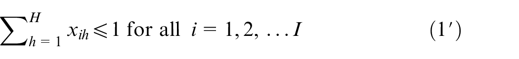
This study addresses a part selection problem for flexible manufacturing systems in which part processing times are controllable to optimize the total cost associated with energy consumption, operational performance, and so on. The problem is to determine the set of parts to be produced, part processing times and the number of tools for each tool type in each period of a planning horizon while satisfying processing time capacity, tool magazine capacity and tool life restrictions. The objective is to minimize the sum of part processing, earliness/tardiness, tool and subcontracting costs. Tool sharing among part types is also considered. After an integer programming model is developed, two types of solution algorithms are proposed, that is, fast heuristics useful when decision time is critical and variable neighborhood search algorithms when solution quality is important. Computational experiments were conducted on a number of test instances and the best fast heuristics are specified, together with reporting how much the variable neighborhood search algorithms improve the fast heuristics.
Introduction
The strategic concept of flexible manufacturing emerged to achieve the two conflicting goals of the manufacturing industry, that is, maximizing productivity and flexibility at the same time. In order to realize the concept, various flexible manufacturing systems (FMSs) were implemented during the last several decades and significant amounts of improvement in the aspects of cost, quality, delivery, and flexibility are reported over the world. Now, the flexible manufacturing concept are being evolved into more advanced ones such as reconfigurable manufacturing, smart manufacturing, and so on.1–6
An FMS can be generally defined as an automated manufacturing system with computer numerical control (CNC) machines, a material handling/storage system and auxiliary facilities, all of which are automatically controlled using a distributed computer control system. Each CNC machine is equipped with an automatic tool changer (ATC) that can automatically interchange cutting tools, which makes an FMS process different part types with high system utilization. However, the capability can be enhanced further when various operational decisions such as planning, scheduling and control are made more efficiently and effectively.
Among various operational problems in FMSs, this study focuses on the part selection problem that determines a set of parts to be produced during an upcoming planning horizon to optimize a certain objective. The problem, alternatively called the batching problem in the literature, is one of pre-release planning that setups parts and tools before an FMS begins to operate. See Stecke, 7 Kouvelis 8 and Tempelmeier and Kuhn 9 for more details on the FMS pre-release planning decisions. Among them, part selection is one of the important ones because the resulting machine loading, resource allocation and scheduling decisions can be made for a given set of parts to be produced.
This study addresses a part selection problem for FMSs in which part processing times are not fixed, but decision variables, called controllable processing times in the literature. Unlike conventional fixed ones, controllable processing times are a practical consideration because there are many situations that job compression is possible while entailing an extra cost, but it is beneficial only if the extra cost is compensated by the gains from earlier job completion. 10 Note that controllable processing times are meaningful in the FMS case when optimizing energy consumption, part precision levels, operational performance, and so on. For example, energy consumption can be optimized by determining appropriate processing times because it is mainly affected by cutting conditions such as cutting depth, feed rate, and cutting speed.11–14 For a given set of parts to be produced during an upcoming planning horizon, the problem is to determine the set of parts to be produced, together with their processing times, and the number of tools required for each tool type in each period of the planning horizon. The objective is to minimize the sum of part processing, earliness/tardiness, tool and subcontracting costs, where part processing costs depend on processing times under different cutting conditions and the other costs are associated with operational performance. As a practical consideration, tool sharing among different part types is also considered.
The part selection problem considered in this study was motivated from a research project that develops an operating system of an FMS with a state-of-the art numerical control machine that can process high strength parts in high precision levels, called the jig center. From the project, we observed that the precision level and operational performance depend highly on the cutting speed, that is, the precision level increases, but the operational performance decreases as the cutting speed decreases. In addition, tooling requirements such as available tool copies, tool lives and tool sharing must be considered for the part selection module to be applicable to the FMS.
An integer programming model is developed to describe the problem mathematically. After the NP-hardness of the problem is proved, two types of solution algorithms are proposed, that is, fast heuristics and variable neighborhood search algorithms. The fast heuristics obtain an initial solution by a greedy algorithm under given initial part processing times and then improve it by simple local search algorithms with processing time adjustment methods, and variable neighborhood search algorithms improve the fast heuristics by escaping from local optimums. Note that the fast heuristics are useful when decision time is critical while variable neighborhood search algorithms are useful when solution quality is important. In fact, this paper is an improved version of Zeid et al. 15 by explaining the fast heuristics more clearly and proposing additional meta-heuristics to obtain better solutions. To test the performance of the algorithms, computational experiments were conducted on a number of test instances and the test results are reported, that is, performance of the fast heuristics and the amounts of improvement obtained by the variable neighborhood search algorithms.
Literature review
This section reviews the research articles on FMS part selection or batching problems after they are classified into single-period and multi-period approaches. The differences from the previous studies are also explained.
Most previous studies consider single-period problems that determine a set of parts to be produced during an upcoming period. Note that the single-period approach must solve a new problem for the next period after the parts selected in the current period are completed. As an earlier study, Hwang 16 suggests a mathematical programming model for the problem that maximizes the number of products to be produced. Due to its impracticality, Hwan and Shogan 17 extend the earlier model by including part importance and machine capacities. Srivastava and Chen 18 propose tabu search heuristics for the capacitated problem that maximizes the weighted number of products, which is extended by Srivastava and Chen 19 that propose a simulated annealing algorithm for the problem with pallet and fixture limitations. Also, Kim and Yano 20 propose a due-date based approach in which that parts are selected using part release priorities determined by approximated schedule information, and Denizel and Sayin 21 consider the problem for the bi-criterion objective of maximizing the number of parts to be produced and minimizing the total tardiness. See Chen et al. 22 and Tabucanon et al. 23 for other single-period models. Besides theses, many articles consider single-period part selection together with machine loading that allocates operations and tools to machines.24–31
To obtain better solutions over a planning horizon with separated periods, the single-period models are extended to multi-period ones that select the parts to be produced in each period of the planning horizon. As an earlier study, Stecke and Toczylowski 32 propose a due-date based model that maximizes the total profit. Also, Lee and Kim 33 consider the problem for the objective of minimizing the sum of earliness, tardiness and subcontracting costs and propose Lagrangean heuristics and later, Zeid et al. 15 extend the earlier problem by considering controllable processing times and propose simple heuristics. As in the single-period case, some articles propose integrated approaches for multi-period part selection and machine loading.34–39 In particular, Shin et al. 39 propose a priority rule based solution approach for multi-period part selection and scheduling in a single-machine FMS with controllable processing times.
As explained earlier, this study improves Zeid et al. 15 by proposing meta-heuristics to obtain better quality solutions. Also, this study is different from Shin et al. 39 in that a more concrete part selection problem with controllable processing times is considered for multi-machine FMSs with tool life constraints and tool sharing. Note that the tooling considerations must be incorporated into the problem to obtain practically feasible solutions that can be applied to on-the-spot FMS operations.
Problem description
The FMS considered in this study consists of multiple identical computer numerical control machines, each of which is equipped with a tool magazine of a limited tool slot capacity. See Figure 1 for an FMS with three machines.
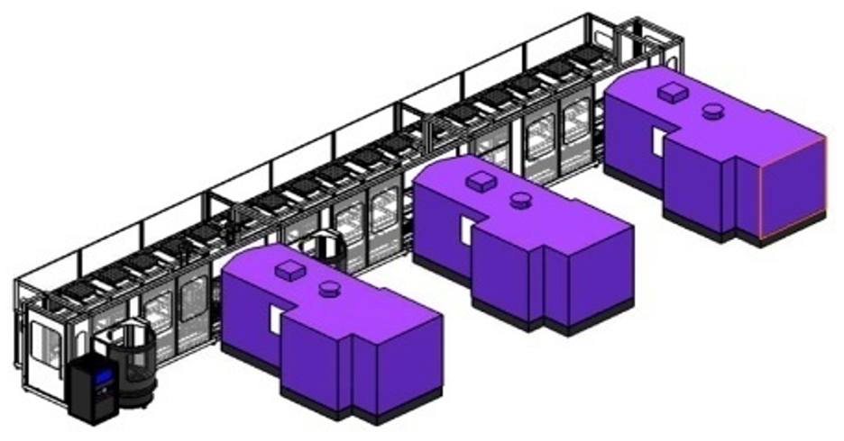
System configuration: an FMS with three machines.
One or more tool types are required to complete a part and a tool type may be used for several part types, called tool sharing. Also, each tool of multiple copies with a limited life is installed on the tool magazines, and each machine, if tooled differently in the tool magazine, can process different part types with negligible setup times. Note that part processing times are discretely controllable, that is, part can be processed according to discretely different processing times with different processing costs, because numerical control machines usually have a finite set of discrete cutting speed modes. It is assumed that part processing times and costs are inverse proportion to each other and given in advance.
For a given set of parts to be produced over an upcoming planning horizon, the problem has three decisions: parts to be produced in each period of the planning horizon; part processing times; and the number of tool copies required for each tool type. Due to system capacities, parts may be subcontracted when not selected within the planning horizon. As the second decision, the processing time of each part is determined by selecting one of the discretely available processing times. Figure 2 shows the part selection and processing time determination decisions. In addition, the number of tool copies for each tool type can be used to estimate the tool requirement for an upcoming planning horizon.
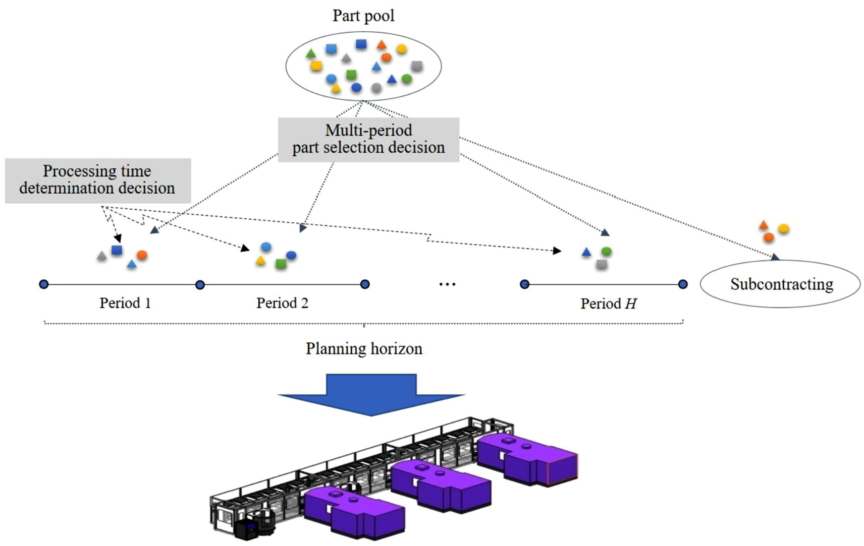
Multi-period part selection and processing time decisions.
The problem has three types of constraints: processing time capacity; tool magazine capacity; and tool life. First, the processing time capacity implies that the total processing time of the parts selected in a period must not be greater than the aggregated one in that period, that is, period length × number of machines × utilization factor. Next, the tool magazine capacity implies that the total number of tool slots required for the parts to be produced in a period must not be greater than the aggregated one, that is, sum of individual tool magazine capacities. Finally, the tool life constraint implies that the total processing time of the selected parts that require a tool type must not be greater than the total life of the tool type, that is, tool life × number of tool copies.
The objective is to minimize the sum of part processing, earliness/tardiness, tool and subcontracting costs. The processing cost of each part, which may vary for different available processing times, implies the cost to process the part. The earliness cost occurs when a part is processed before its due-date, for example, inventory holding cost, while the tardiness cost occurs if processed after its due-date. It is assumed that the due-date of each part is specified by a period in the planning horizon, that is, the part is due at the end of the period. For example, suppose that the due-date of a part is period 4 in a 10-period problem. Then, an earliness cost occurs if the part is assigned to period 3, while a tardiness cost occurs if the part is assigned to period 5. Also, the tool cost implies the total cost of the tools required to process the selected parts, which is directly proportional to the number of required tools. Finally, the subcontracting cost occurs when parts are not selected within the planning horizon. To maximize the system utilization up to its processing time capacity, it is assumed that the subcontracting cost of a part is always greater than the maximum earliness/tardiness cost of the part.
The problem can be formulated as an integer programming model. Before presenting the model, the notations are summarized below.
Indices
Parameters
where
Decision variables
Now, the integer programming model is given below. Note that the following model is an extended one of Lee and Kim 33 by additionally representing controllable processing times and additional tooling considerations.
subject to
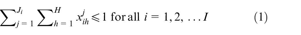
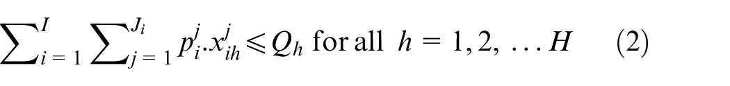
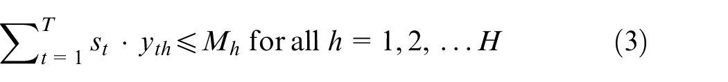
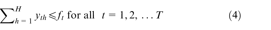
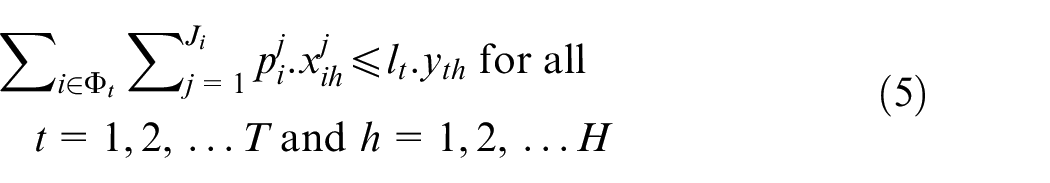
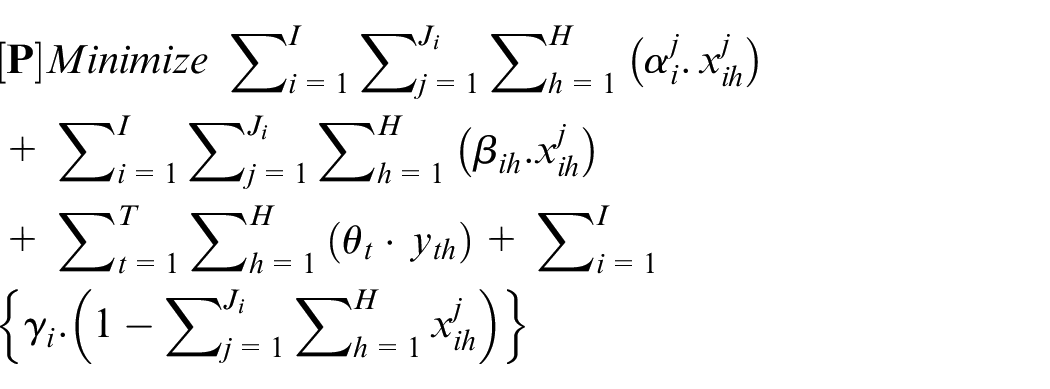
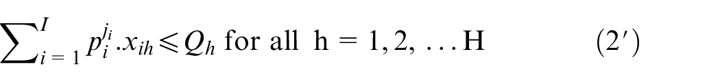
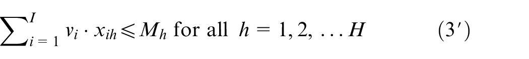
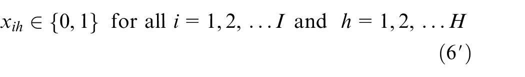
The objective represents the sum of part processing, earliness/tardiness, tool and subcontracting costs over the planning horizon. Constraint set (1) ensures that each part is selected within the planning horizon or subcontracted, together with determining its processing time. Constraint sets (2) and (3) represent the processing time and the tool magazine capacities, respectively. Also, a constraint set (4) represents the number of available tool copies for each tool type and constraint set (5) represents the tool life restrictions. Finally, the remaining (6) and (7) represent the conditions of decision variables.
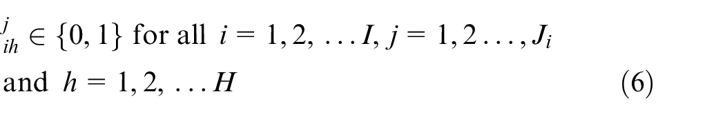
It is possible to solve the problem [P] directly using an integer programming software package, but it requires excessive computation time for large sized instances. Note that the problem [P] is NP-hard because it can be reduced to the multi-period part selection problem of Lee and Kim
33
by fixing part processing times and relaxing the tooling constraints (4) and (5) while removing the part processing and tool costs in the objective function. Formally, let
subject to
Lee and Kim 33 show that the problem [RP] can be transformed into the generalized assignment problem with additional constraints and it can be seen that the problem [P] considered in this study is NP-hard because the special case [RP] is proved to be NP-hard. Therefore, instead of the optimal solution approach with limited applications, the heuristic approach is adopted in this study.
Solution algorithms
This section presents two types of solution algorithms: fast heuristics that can be used when computation time is critical and variable neighborhood search algorithms when solution quality is important.
Fast heuristics
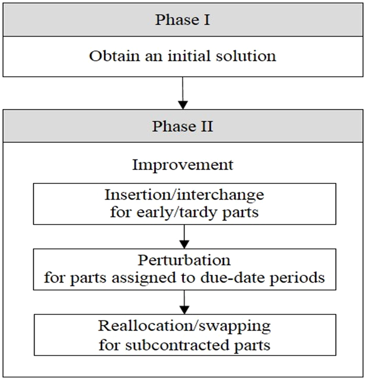
The fast heuristics consist of two stages: (a) obtaining an initial solution; and (b) improvement. Figure 3 shows an overview of the fast heuristics.
Fast heuristics: overview.
Stage I: Obtaining an initial solution
After the processing time of each part is fixed to its longest one, an initial solution is obtained by a greedy algorithm that sorts the parts in the non-increasing order of subcontracting costs and according to the sorted list, they are assigned to the period with the smallest earliness/tardiness cost without violating the constraints. The detailed procedure is given below. Ties are broken arbitrarily.
Step 1. Sort the parts in the non-increasing order of subcontracting costs
Step 2. Set the processing time of each part to its longest available one, that is,
Step 3. From the first to the last part in the sorted list, find the period
Stage II: Improvement
The initial solution is improved by three consecutive steps: insertion/interchange for early/tardy parts, perturbation for the parts assigned to their due-date periods and reallocation/swapping for subcontracted parts. The details are explained below.
Step 1. Insertion/interchange for early/tardy parts
Let
where
Insertion
The insertion method improves the current solution by removing a part in each of
In the insertion method, the following methods are tested to select a neighborhood solution.
BI (best improvement): insert the part to the best feasible period that improves the current solution
HI (hybrid improvement): insert the current part to the better one of the first and the best feasible periods that improve the current solution
For the two methods, the neighborhood solutions for each part are generated as follows. Let
Case 1: If the current part
Case 2: Otherwise, generate other neighborhoods that can improve the current solution without violating the constraints by inserting part
In the case of part
In the case of parts in
MCI (minimum cost increase): select part
MTD (maximum time decrease): select part
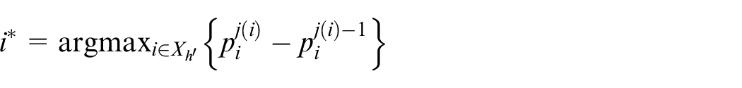
CTR (cost/time ratio): select part
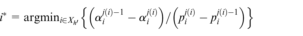
To illustrate the insertion method, consider a 5-period example for five parts each of which has three available processing times. The data are summarized in Table 1.
Insertion method: example.
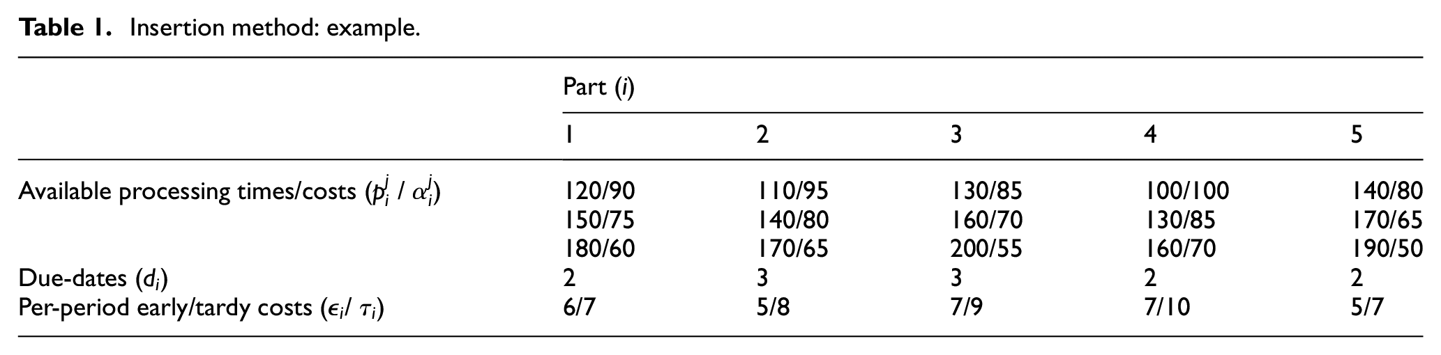
Let the current solution be
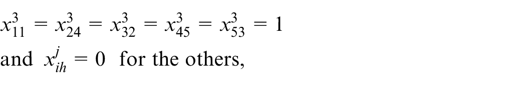
that is,

and then it can be reallocated to periods 1, 2, 3, and 4 if all the constraints are satisfied. Among them, consider the case that it is reallocated to period 2. If the reallocation is feasible and improves the current solution, we obtain a neighborhood solution (Case 1). Otherwise, another neighborhood solution can be obtained if an improved feasible solution can be obtained by changing its processing time (Case 2(a)), for example, from
Interchange
After the insertion is done, the current solution is improved further by interchanging early and tardy parts while adjusting the part processing times. Specifically, the parts in
Step 2. Perturbation for parts assigned to their due-date periods
The perturbation step is done for the parts assigned to their due-date periods. Let
The perturbation is done from the first to the last due-date period, that is, from
The detailed perturbation procedure is given below. Ties are broken arbitrarily.
Set
Find the set
From the smallest to the largest indexed part in
Check if the solution can be improved by interchanging the current part and the parts assigned to other periods in the non-increasing order of their earliness/tardiness costs while adjusting the processing times of the current part and the parts assigned to the period to which the current part is assigned.
If an improved solution is obtained, update the solution. Set the current part to the next indexed one and go to Step 3(a).
If
Step 3. Reallocation/swapping for subcontracted parts
In the reallocation method, the current solution is improved by sorting the subcontracted parts in the non-increasing order of subcontracting costs and then reallocating each part to the first feasible period among those in the non-decreasing order of earliness/tardiness costs while adjusting the processing times of relevant parts explained earlier. After the reallocations, the swapping method improves the current solution by interchanging the remaining subcontracted parts in the non-increasing order of subcontracting costs and the non-subcontracted parts in the non-increasing order of earliness/tardiness costs while adjusting the processing times of the relevant parts.
Variable neighborhood search algorithms
This section explains the variable neighborhood search (VNS) algorithms to improve the fast heuristics. The VNS algorithm, one of well-known meta-heuristics that have been applied to various optimization problems, is based on the systematic change of neighborhood solution within a local search algorithm for the purpose of escaping from local optimums. See Hansen and Mladenović 40 and Hansen et al. 41 for details on the basic VNS and its variants.
The VNS algorithms proposed in this study consists of four steps: (a) obtaining an initial solution; (b) shaking that generates neighborhood solutions and selects one of them; (c) local search that improves the selected neighborhood solution; and (d) termination. Figure 4 shows an overview of the VNS algorithms. As can be seen in the figure, the shaking and local search improvement steps are repeatedly done until the termination condition is satisfied and the algorithms are terminated when the iteration count reaches a predetermined limit
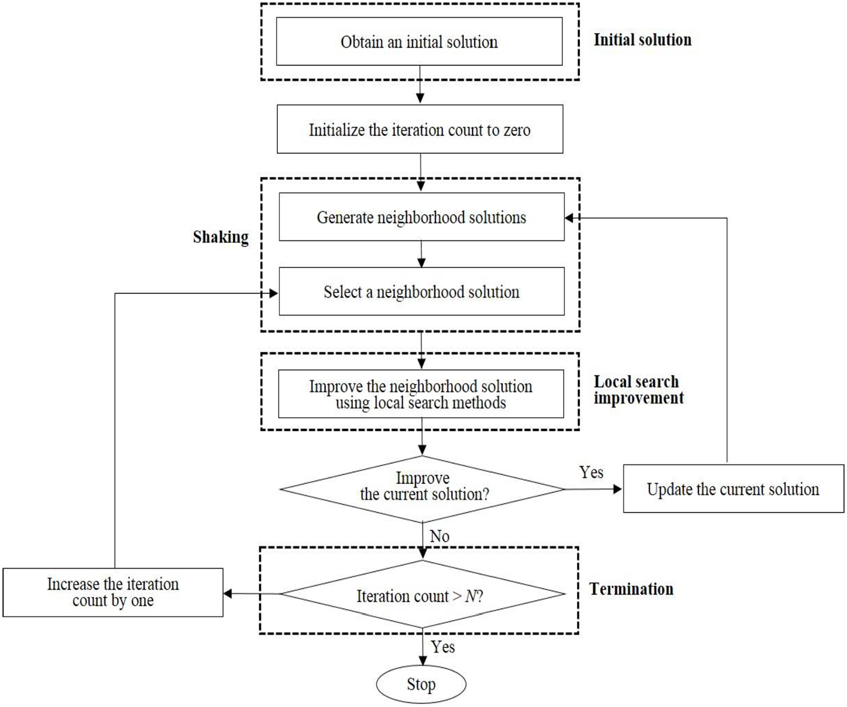
Variable neighborhood search algorithms: overview.
A solution is represented by a
where ⌈·⌉ denotes the smallest integer that is greater than or equal to · and
Obtaining an initial solution
An initial solution is obtained using the greedy algorithm used by the fast heuristics, that is, parts are sorted in the non-increasing order of subcontracting costs and according to the sorted list, they are assigned to the period with the smallest earliness/tardiness cost without violating the constraints.
Shaking
The shaking is done to resolve any local optima traps by changing neighborhood solutions in a systematic way. As in the ordinary VNS algorithm, the shaking step consists of two parts: (a) generating neighborhood solutions; and (b) selecting one of them. The neighborhood solutions are generated using the interchange method explained earlier, that is, interchanges of early and tardy parts while adjusting the processing times. After the neighborhoods are generated, the selection is done randomly to avoid cycling that may occur if a deterministic rule is used, that is, random jump. Note that three VNS algorithms are tested according to the three processing time adjustment methods in the neighborhood generation, that is, MCI, MTD and CTR.
Local search improvement
This step improves the neighborhood solution selected in the shaking step. For this purpose, the three improvement methods of the fast heuristic approach are sequentially used, that is, insertion/interchange for early/tardy parts, perturbation or the parts assigned to their due-date periods and reallocation/swapping for subcontracted parts.
Computational results
This section presents the test results for the two types of solution algorithms. The algorithms were coded in C and the tests were conducted using a PC with Intel Core i7 CPU at 3.40GHz with 8GB RAM memory.
The first test was done to compare the 6 fast heuristics, that is, six combinations of two insertion/interchange methods (BI and HI) and three processing time adjustment methods in the neighborhood generation (MCI, MTD and CTR). The performance measures to evaluate the results are: (a) percentage gaps from the optimal solution values for small sized test instances, defined for a test instance as

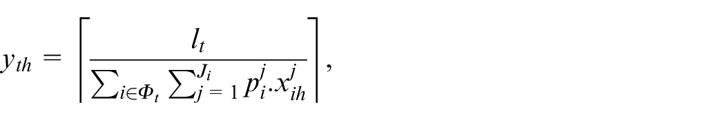
where

where
For the experiment on small sized instances, we generated 60 instances with 5 periods randomly, that is, 10 instances for each of six combinations of three levels for the number of parts (20, 30, and 50) and two levels of the number of tool types (
Number of available processing times
Processing times
Due-dates
Processing costs
Per-period earliness and tardiness costs
Tool cost (
Subcontracting costs =
Number of available tool copies
Tool life
Set of parts that require a tool type (
Number of slots required for each tool type
Aggregated processing time capacities (
Aggregated tool magazine capacities (
Test results for the small sized instances are given in Table 2 that shows the number of instances that the CPLEX gave optimal solutions within 1 h, CPU seconds of the CPLEX and the average percentage gaps of the 6 fast heuristics. Note that the CPU seconds are not reported because the fast heuristics solved all the test instances within 3 s. It can be seen from the table that the CPLEX could not always give the optimal solutions for the small sized test instances with 30 and 50 parts. In fact, it was found from additional experiments that the CPLEX could not give the optimal solutions for the test instances with 10 and 15 periods within 3600 s. Also, Table 2 shows that all the fast heuristics gave near optimal solutions within 2% gaps although no one dominates the others.
Test results for fast heuristics: small sized test instances.
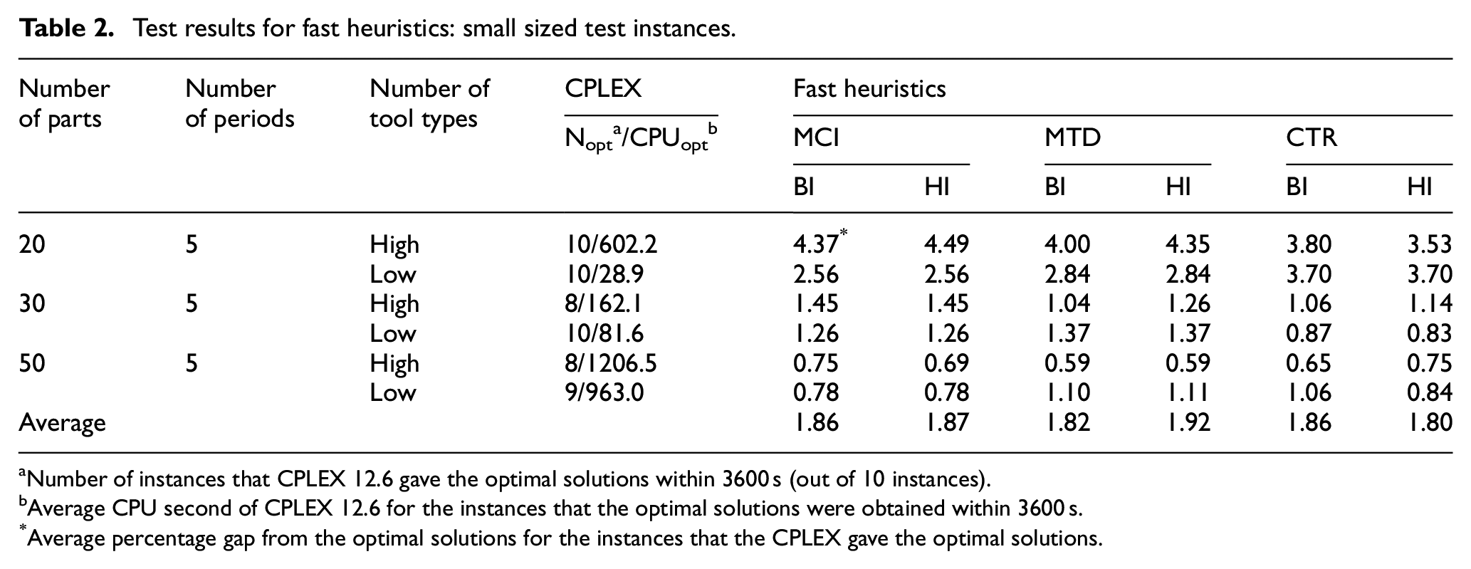
Number of instances that CPLEX 12.6 gave the optimal solutions within 3600 s (out of 10 instances).
Average CPU second of CPLEX 12.6 for the instances that the optimal solutions were obtained within 3600 s.
Average percentage gap from the optimal solutions for the instances that the CPLEX gave the optimal solutions.
For the experiment on medium-to-large sized instances, we generated 240 additional instances randomly, that is, 10 instances for each of 24 combinations of four levels for the number of parts (20, 30, 50, and 100), two levels for the number of periods (10 and 15) and two levels of the number of tool types (high and low). The data were generated using the method explained earlier.
Table 3 shows the average relative performance ratios of the 6 fast heuristics. The CPU seconds are not reported because they solved all the test instances within 20 s. It can be seen from the table that the fast heuristics with CTR are better than the others. This is because CTR considers both costs and processing times when adjusting part processing times in the neighborhood generation method. Note that MCI and MTD consider only one factor, that is, cost or processing time. However, as in the results for small sized instances, there is no significant difference between BI and HI. Also, to show the effects of the numbers of parts, periods and tool types and the combinations of insertion/interchange and processing time adjustment methods on the solutions, an analysis of variance (ANOVA) was done using the relative performance ratio values for all test instances and the result given in Table 4 shows that the solutions are significantly affected by the insertion/interchange and processing time adjustment methods. This implies that the two decisions are important ones that must be made efficiently in the FMS part selection.
Test results for fast heuristics: medium-to-large sized test instances.
(a) Relative performance ratios.
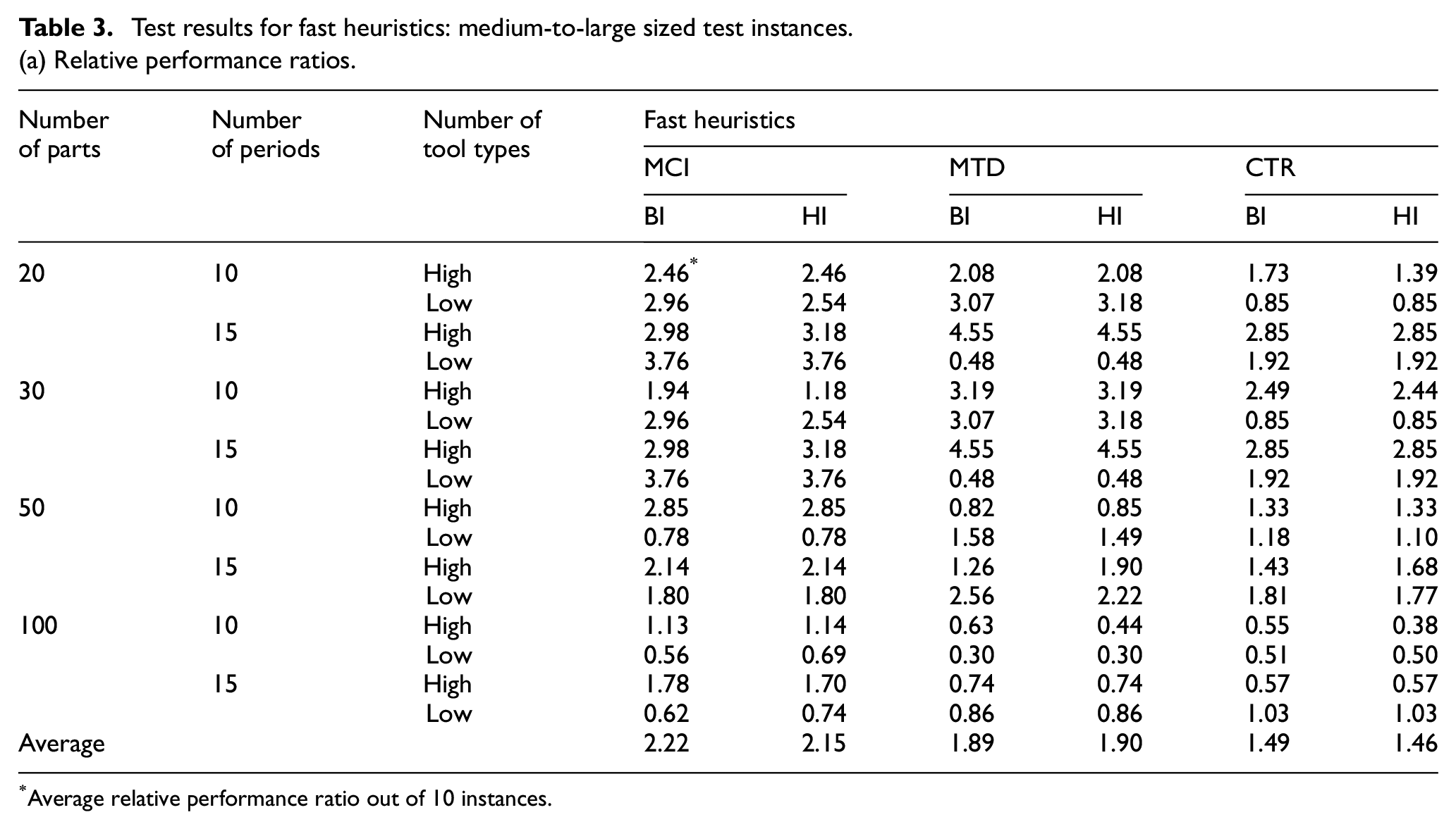
Average relative performance ratio out of 10 instances.
(b) CPU seconds.
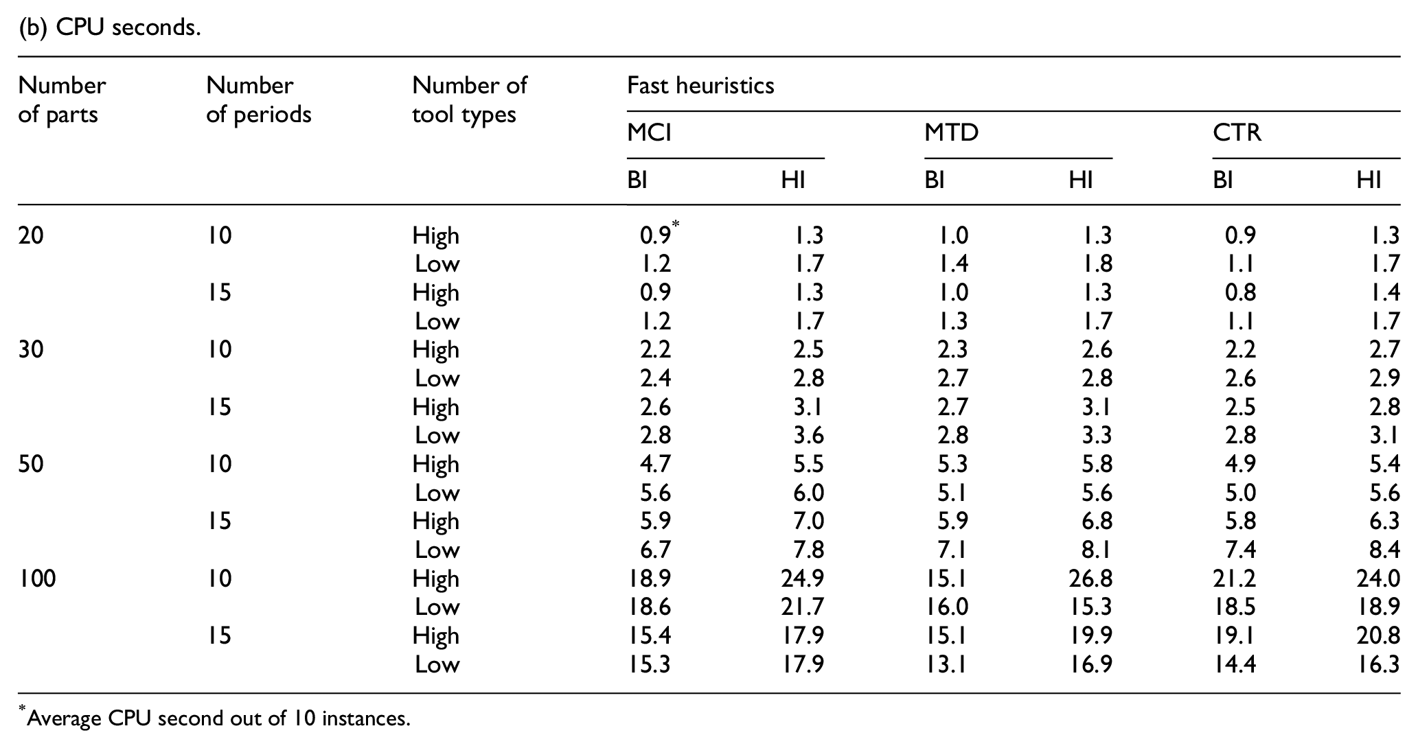
Average CPU second out of 10 instances.
Analysis of variance for the effects of four factors.
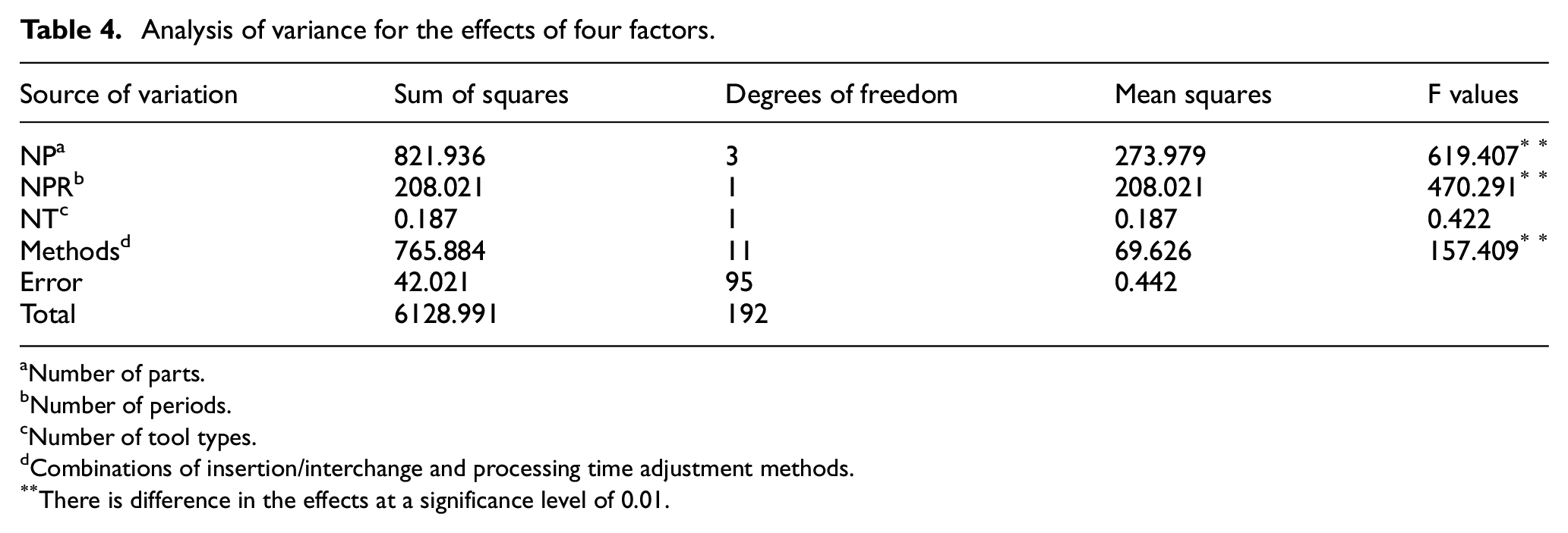
Number of parts.
Number of periods.
Number of tool types.
Combinations of insertion/interchange and processing time adjustment methods.
There is difference in the effects at a significance level of 0.01.
The last experiment was done to test the VNS algorithms with different processing time adjustment methods (MCI, MTD and CTR), where the algorithms were terminated when the iteration count (
Test results for VNS algorithms.
(a) Average percentage gaps.
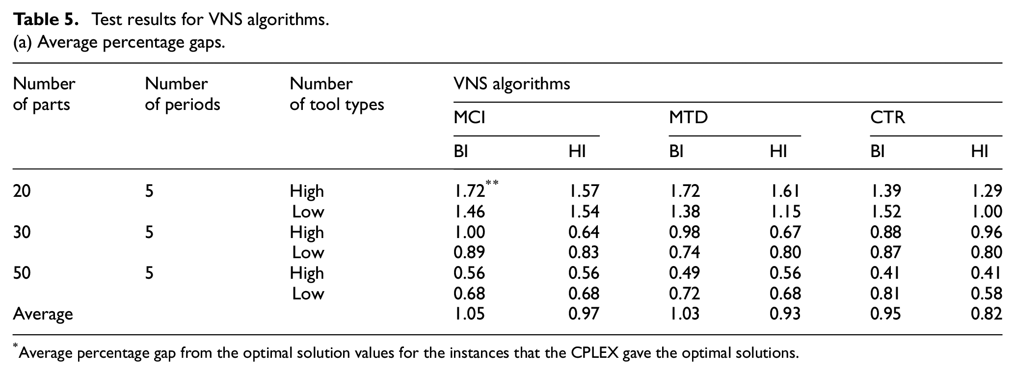
Average percentage gap from the optimal solution values for the instances that the CPLEX gave the optimal solutions.
(b) Percentage improvement over fast heuristics.
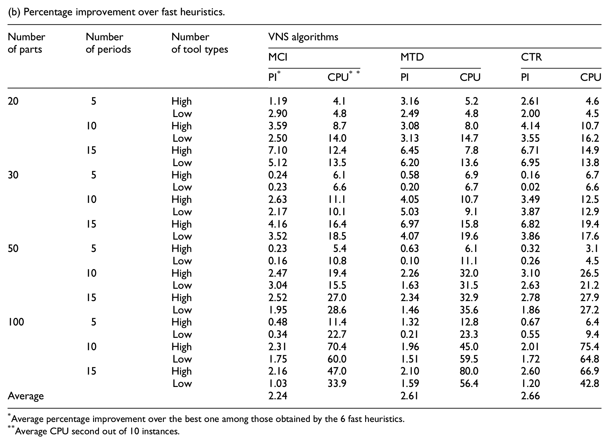
Average percentage improvement over the best one among those obtained by the 6 fast heuristics.
Average CPU second out of 10 instances.
Results of the paired t-tests for VNS algorithms.
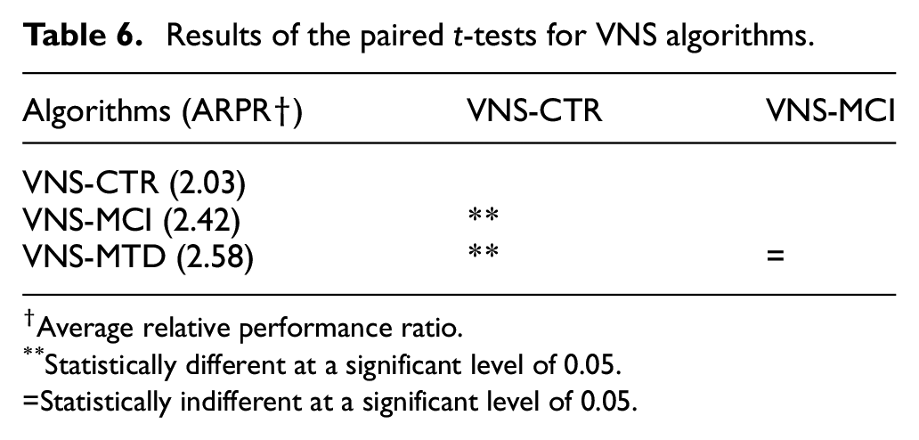
Average relative performance ratio.
Statistically different at a significant level of 0.05.
=Statistically indifferent at a significant level of 0.05.
Concluding remarks
This study considered a multi-period part selection problem for FMSs in which part processing times are controllable to optimize energy consumption, part precision levels, operational performances, and so on. Tool sharing among different part types is also considered to obtain practically feasible solutions applicable to real FMSs. The problem is to determine the set of parts to be produced in each period, part processing times and the number of copies for each tool type while satisfying the processing time capacity, tool magazine capacity and tool life constraints. The objective is to minimize the sum of part processing, earliness/tardiness, tool and subcontracting costs. After an integer programming model was proposed, together with proving its NP-hardness, two types of heuristics were proposed: fast heuristics useful when computation time is critical and variable neighborhood search algorithms useful when solution quality is important. Computational experiments were done on various test instances and the results are as follows. First, among the 6 fast heuristics, the ones with the CTR (cost/time ratio) based processing time adjustment method work better than the other, and gave near optimal solutions for small sized test instances, that is, within 2% from the optimal solution values in the overall average. Second, the VNS algorithms improve the fast heuristics significantly, that is, 2.66%, 2.61%, and 2.24% for VNS-CTR, VNS-MCI, and VNS-MTD, respectively. Finally, as in the test results of the fast heuristics, VNS-CTR performs the best.
This study can be extended as follows. First, the problem can be extended to stochastic ones with uncertain processing times, costs, machine/tool breakdowns, and so on. Second, it is needed to integrate the part selection model with other FMS operation problems such as machine loading and scheduling.
Footnotes
Declaration of conflicting interests
The author(s) declared no potential conflicts of interest with respect to the research, authorship, and/or publication of this article.
Funding
The author(s) disclosed receipt of the following financial support for the research, authorship, and/or publication of this article: This work was supported by the Technology Innovation Program funded by the Ministry of Trade, Industry & Energy, Korea Government. (Grant code: 10052978-2015-4, Title: Development of a jig-center class 5-axis horizontal machining system capable of over 24 hours continuous operation)