A nested circle-fitting method for micro-hole centering and its application in electrochemical deburring

Abstract

To solve these problems (i.e. the accuracy rate and stability of the centering) of enabling secondary machining of micro-holes with a size of 0.1 to 1 mm in high-performance metal alloy parts, a non-standard nested circle-fitting least-square method, with a linear constraint passing through the center (least square method with linear constraint [LSLC]), is proposed in this article. The experimental results show that the center of the circle is fitted with a maximum deviation of ±1.5 µm and good fitting precision, compared to other existing approaches. At the same time, the accuracy rate is increased by at least 20%, delivering a result of more than 99%, so the accuracy of the fitting and the stability of the centering are significantly improved. Finally, the new method is applied in actual micro-hole electrochemical deburring study. With the overall goal of ensuring centering, a rough-and-fine deburring process has been explored. On the premise that the hole is not expanded, the burrs have been quickly and completely removed, and machined surface roughness, R_a, has also reduced from 1.2 to 0.52 µm. The experiment has provided concrete validation of the feasibility of the nested circle-fitting method we have proposed.

Introduction

The creation of high-performance metal alloy parts with micro-holes that are characteristically between 0.1 and 1 mm is an important production requirement in advanced micro-manufacturing. Applications here include needle-valve oil nozzles for automotive engines, ¹ film-cooling holes in airplane engines, ² and so on. However, the current micro-electro-discharge machining (micro-EDM) approach to the production of micro-holes results in micro-cracks and recasting layers on the inner wall of the hole. ³ This can cause the alloy parts to break during operation, raise their susceptibility to fatigue, and impact their working life. Alongside of this, burrs at the bottom can change the cross-section of the micro-hole, making it an uneven circle and affecting flow coefficients and injection performance. As a result of all this, secondary machining of the micro-holes has been undertaken using electrochemical deburring. ⁴ This can substantially improve the surface quality and shape precision of the parts. ⁵ However, centering between the micro-hole and the electrode is a key aspect of the secondary machining and this is not a straightforward process.

Existing centering methods mainly involve either contact or non-contact approaches. Contact methods include the dial-indicator method, the three-point method, ⁶ and the orthogonal-point electrical contact method. ⁷ Non-contact methods involve things like laser alignment ⁸ and image centering. ⁹ Each of these methods has its own unique advantages, but there are numerous restrictions on how they can be used. Thus, in the dial-indicator method, shifting forces on the probe contact can easily cause the dial-indicator holder to slip. This can impact the accuracy of the centering and lead to faulty installations. The three-point method is a form of circle fitting that involves measuring the position of any three points on the edge of the micro-hole. The orthogonal-point electrical contact method requires a moving trace of the thin electrode from a left contact point to a right contact point (Line 1), and from an upper contact point to a lower contact point (Line 2), thus making the traces orthogonal. The circle can then be fitted by sensing the contact points using low voltages. When non-standard circular micro-holes are fitted using the three-point method and the orthogonal-point electrical contact method, it is difficult to ensure the accuracy of the centering when there are any burrs or distortions in the holes, and micro-electrodes also lack rigidity. Laser approaches involve installing a laser emitter/receiver on an electrode and the micro-hole, respectively. This can determine the center according to calculated center deviations. However, as the micro-holes and electrodes are small, probe installation can be difficult. This makes this method ineffective for micro-hole centering if the holes have a diameter of less than 1 mm. Image-centering approaches require the implementation of an imaging system to capture the images of two nested circular components. Any positional offset of the nested center is obtained through image processing. The position of the components is then adjusted to complete the centering. This method is both rapid and contact-free. It is also applicable to the microscopic centering of micro-holes and electrodes. However, for this approach to work, the fitting of the nested circles is a key factor that can affect the precision, accuracy, and stability of the microscopic centering.

Commonly used approaches to circular fitting include the traditional least-square (TLS) method,^10,11 the randomized Hough-transform method,^12,13 a circle-fitting method that involves determining the threshold and updating the step length,^14,15 the radius constrained least-square method,^16–18 and the region-constrained least-square (RCLS) method.^19–21 When using image centering, the edge of the actual image is a non-standard nested circle with noise. This means that, if there is noise near the extracted feature point, the TLS fitting result may not reflect the actual situation, leading to inaccuracies in the centering. The randomized Hough-transform method is often used for detecting standard circles, but it has a high non-detection rate for non-standard circles.

There has been a lot of research addressed to overcome the above-mentioned difficulties. For example, Milan et al. ¹⁴ and Li and Liu. ¹⁵ have proposed a circle-fitting method that involves determining thresholds and updating step lengths. A circle-fitting measurement function is first of all defined. Updates in step length are then repeatedly performed, with the center point coordinates being re-calculated and the radius updated, until the updated step length is smaller than a set threshold. This method is fast and accurate for single circles and is very resistant to noise. However, it is not able to handle the interference arising from adjacent circles, so it cannot be used for nested circle fitting.

During the machining of workpieces, the circle radius can be known or obtained in advance by using other measurement methods. Researchers such as Psiaki et al., ¹⁶ Nattila et al., ¹⁷ and Majczyna et al. ¹⁸ have proposed a circle-fitting method that is based on a constrained radius. This method is effective at improving fitting precision and accuracy but is not suitable for non-standard nested circle fitting where there are burrs and distortions, and an unknown radius.

Other researchers, including Seers and Hodgetts, ¹⁹ Fox et al., ²⁰ and Kong et al., ²¹ have proposed an RCLS fitting method. This method employs a center-circle region constraint to increase the ratio between the feature edge points and total edge points in an image. This serves to substantially reduce the edge noise and improve the precision and fitting accuracy of the circle. It is also applicable to the fitting of non-standard nested circles. However, it uses a chain-tracing structure by scanning the center. As a result, over time, invalid cases cumulatively increase and the accuracy and performance quality are reduced. In addition, recurrent square and square root operations increase the computational complexity, which makes the approach time-consuming and less than ideal for real-time applications.

The above-mentioned literatures on the fitting of the nested circles in microscopic centering show that the randomized Hough-transform method has a high non-detection rate for non-standard circles. The circle-fitting method that involves determining the threshold and updating the step length is not able to handle the interference arising from adjacent circles, so it cannot be used for nested circle fitting. The radius constrained least-square method is not suitable for non-standard nested circle fitting where there are burrs and distortions, and an unknown radius. And the RCLS method is time-consuming and less than ideal for real-time applications.

To sum up, a range of issues, including burrs at the bottom and non-standard nested circular cross-sections with unknown radius, mean that current approaches to the centering and circle fitting of micro-holes in metal alloy parts struggle to ensure the accuracy and stability of the centering while still satisfying the requirements of real-time performance. In this article, we will be setting out a new approach that is based on microscopic imaging technology. By analyzing the features of nested circles in an image, we will be introducing the constraint of a straight line through the center of the circle to be fitted. On the basis of this, we will then propose a non-standard nested circle-fitting least-square method with a linear constraint passing through the center. After this, we shall produce the results of a fitting comparison experiment that we conducted to verify the effectiveness of our proposed method. We shall also be reporting on how the method was applied in actual micro-hole electrochemical deburring experiments. During these experiments, we examined the deburring process to verify the feasibility of our fitting method for real-time micro-hole electrochemical deburring and the extent to which it offers a way of improving the manufacture of advanced alloy components.

The nested circle-fitting method based on a least-square method with a linear constraint passing through the center

In existing circle-fitting algorithms, it is difficult to meet the needs of real-time performance while ensuring centering accuracy when fitting non-standard nested circles with noise and distortion. In this article, we propose a nested circle method that is based on the least-square method but with a linear constraint passing through the center. The proposed algorithm is designed to solve various problems outlined above. The solution includes things such as image preprocessing, electrode inner-circle filtering, electrode outer-circle fitting, intersected circle drawing, calculation of intersection point centers, constrained line drawing, and circle fitting. The fitting process is shown in Figure 1 and can be described as follows.

• 1. Image preprocessing.

A microscopic system is used to collect and correct images of micro-holes and the corresponding hollow electrode. The diameter of the micro-hole shown in Figure 1(a) is about 0.5 mm. The image is successively binarized, noise-removed, edge-extracted, image-marked, and preprocessed in other ways. The resulting image is shown in Figure 1(b). It should be noted that image marking not only facilitates the filtering of the inner circle of the electrode but also helps to avoid interference between adjacent circles. This enhances its scope to improve fitting speed and fitting accuracy.

• 2. Electrode inner-circle filtering and electrode outer-circle fitting.

The inner circle of the electrode can produce interference data and affect the fitting outcome. This needs to be filtered in that case (see Figure 1(c)). A molding tube is selected as the hollow electrode, with the outer circle being close to a standard circle. Direct implementation of the TLS method provides a fast fitting speed and high precision. The fitted circle center of the outer circle (Circle 1) is marked by O₁, as shown in Figure 1(d). Due to the presence of burrs in micro-holes and various kinds of noise that cannot easily be removed, directly fitting the edge of the micro-hole using the TLS method may result in incorrect fitting results (see Figure 1(h)).

• 3. Intersected circle drawing.

Circles with different radii intersecting with the edges of the micro-hole are drawn with a center of O₁. The corresponding intersection points are F₁, G₁, F₂, G₂, F_i, and G_i $(i=1,2,3,\dots ,n)$ , as shown in Figure 1(e). Note in particular that F_i and G_i are symmetrical with respect to O₁; n is the number of intersections. The radius range of the micro-hole in the known workpiece is [a, d]. Let the radius of the drawing circle be r_i∈ [a, d], where r_i can be expressed as a+i·Δ, Δ = (d – a)/n. The intersection points F_i and G_i will then satisfy equation (1)

$$\begin{array}{c}\left[\begin{array}{cc}{x}_{11}-x_1\hfill & y_{11}-y_1\hfill \\ \multicolumn{1}{c}{⋮}& ⋮\hfill \\ \multicolumn{1}{c}{x_{\mathrm{ii}}-x_1}& y_{\mathrm{ii}}-y_1\hfill \\ \multicolumn{1}{c}{⋮}& ⋮\hfill \\ \multicolumn{1}{c}{x_{\mathrm{nn}}-x_1}& y_{\mathrm{nn}}-y_1\hfill \end{array}\right]\hfill \\ \left[\begin{array}{ccccc}{x}_{11}-x_1\hfill & \cdots \hfill & x_{\mathrm{ii}}-x_1\hfill & \cdots \hfill & x_{\mathrm{nn}}-x_1\hfill \\ \multicolumn{1}{c}{y_{11}-y_1}& \cdots \hfill & y_{\mathrm{ii}}-y_1\hfill & \cdots \hfill & y_{\mathrm{nn}}-y_1\hfill \end{array}\right]=\hfill \\ \left[\begin{array}{ccccc}{a}^2\hfill & \cdots \hfill & \cdots \hfill & \cdots \hfill & \cdots \hfill \\ \multicolumn{1}{c}{⋮}& {(a+\Delta )}^2\hfill & \ddots \hfill & \ddots \hfill & ⋮\hfill \\ \multicolumn{1}{c}{⋮}& \ddots \hfill & \ddots \hfill & \ddots \hfill & ⋮\hfill \\ \multicolumn{1}{c}{⋮}& \ddots \hfill & \ddots \hfill & {[a+(n-1)\Delta ]}^2\hfill & ⋮\hfill \\ \multicolumn{1}{c}{\cdots }& \cdots \hfill & \cdots \hfill & \cdots \hfill & {(a+n\Delta )}^2\hfill \end{array}\right]\hfill \end{array}$$

(1)

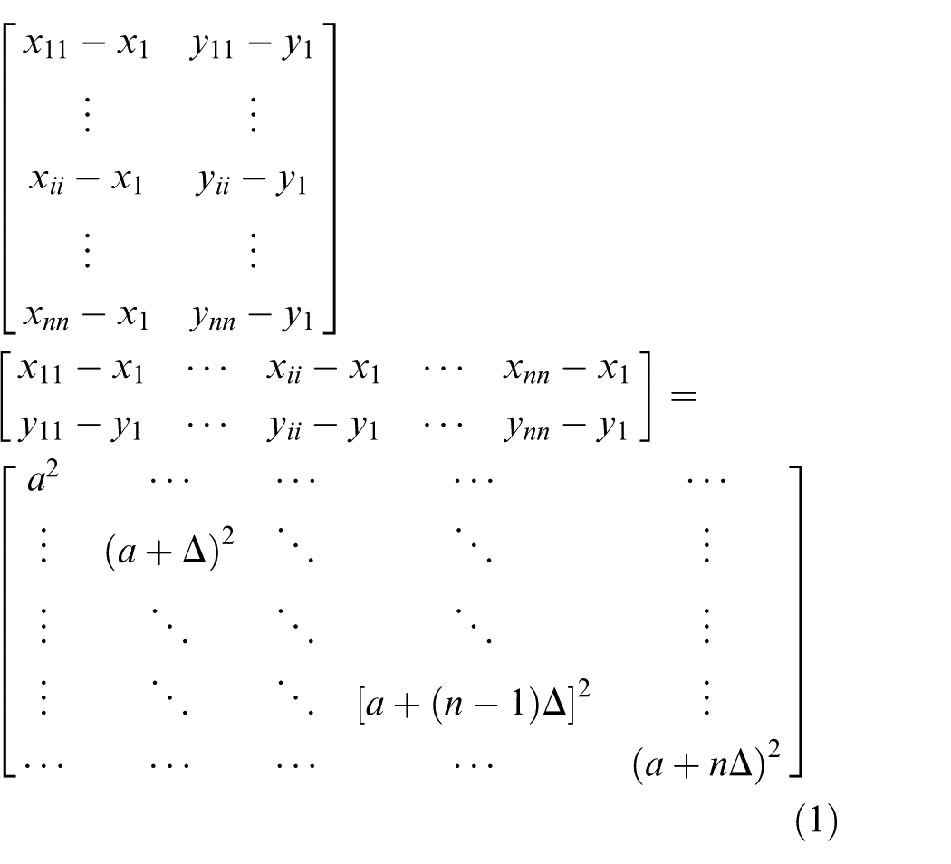
where (x₁, y₁) represents the center O₁ of Circle 1 and (x_ii, y_ii) represents an arbitrary point along the edge of the micro-hole.

• 4. Calculation of the intersection center and the drawing of the constrained straight line passing through the center.

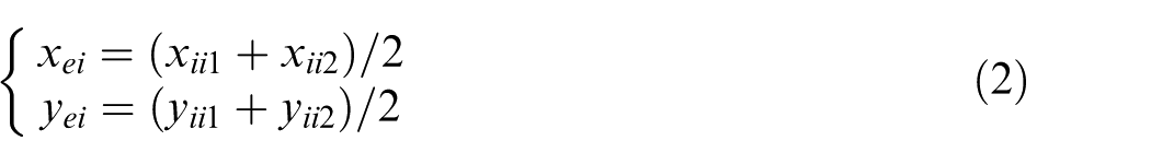
Each set of corresponding intersection points F_i(x_ii1, y_ii1) and G_i(x_ii2, y_ii2) can be obtained from equation (1). The coordinates (x_ei, y_ei) of each point corresponding to the middle point e_i of the intersection point are calculated according to equation (2), as illustrated in Figure 1(f)

$$\{\begin{array}{c}{x}_{\mathrm{ei}}=(x_{\mathrm{ii}1}+x_{\mathrm{ii}2})/2\hfill \\ \multicolumn{1}{c}{y_{\mathrm{ei}}=(y_{\mathrm{ii}1}+y_{\mathrm{ii}2})/2}\end{array}$$

(2)

Assuming that the slope of the constrained straight line named as M, which passes through the center, is k, and that the intercept is b, then k and b will satisfy equation (3)

$$\left[\begin{array}{cc}n\hfill & \sum _{i=1}^n{x}_{\mathrm{ei}}\hfill \\ \multicolumn{1}{c}{\sum _{i=1}^n{x}_{\mathrm{ei}}}& \sum _{i=1}^n{x}_{\mathrm{ei}}^2\hfill \end{array}\right]\left[\begin{array}{c}b\hfill \\ \multicolumn{1}{c}{k}\end{array}\right]=\left[\begin{array}{c}\sum _{i=1}^n{y}_{\mathrm{ei}}\hfill \\ \multicolumn{1}{c}{\sum _{i=1}^n{x}_{\mathrm{ei}}{y}_{\mathrm{ei}}}\end{array}\right]$$

(3)

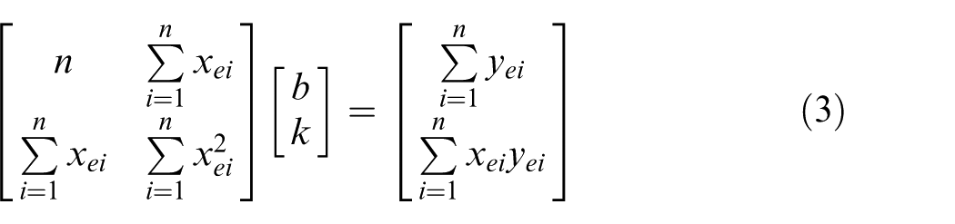
Equation (3) is solved by least-square method, and the constrained straight-line M that passes through the center can now be obtained (see Figure 1(f)). If the F_i and G_i happen to encounter the burr, then e_i will be offset. However, the number of selected sampling points is a big number. When the number of selected sampling points is greater than 600, the residual errors of the slope (k) and the intercept (b) of the constrained straight-line M are less than 10^–6, respectively. Thus, the results meet actual requirements, and the algorithm is still valid. The linear constraint that passes through the center obviates the effects of noise and burrs, thus ensuring the fitting accuracy of the nested outer circle.

• 5. Micro-hole edge fitting.

In Figure 1(g), the edge of the micro-hole (nested outer circle) is fitted as Circle 2 and the center of the circle is O₂. This being the case, the objective function of the circle fitting based on the linear constrained least-square method is shown in equation (4)

$$C_q=\sum _{p=1}^N{(\sqrt{{(x_0-x_p)}^2+{(y_0-y_p)}^2}-R)}^2+\lambda f(x_0,y_0)$$

(4)

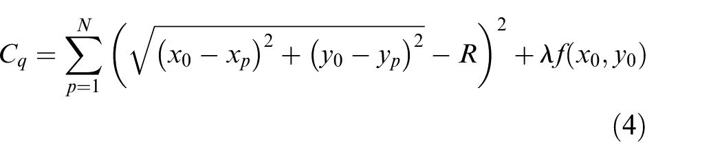
where (x_p, y_p) are the coordinates of a selected sampling point on the edge of the micro-hole, N is the number of selected sampling points, (x₀, y₀) are the center coordinates of Circle 2, R is the radius of Circle 2, λ is a Lagrangian multiplier, and f(x₀, y₀) is the equation for the center-constrained line M, which is f(x₀, y₀) = y₀–kx₀–b, and $q=1,2,3,\dots ,V$ (where V is the number of objective functions C_q).

Figure 1.

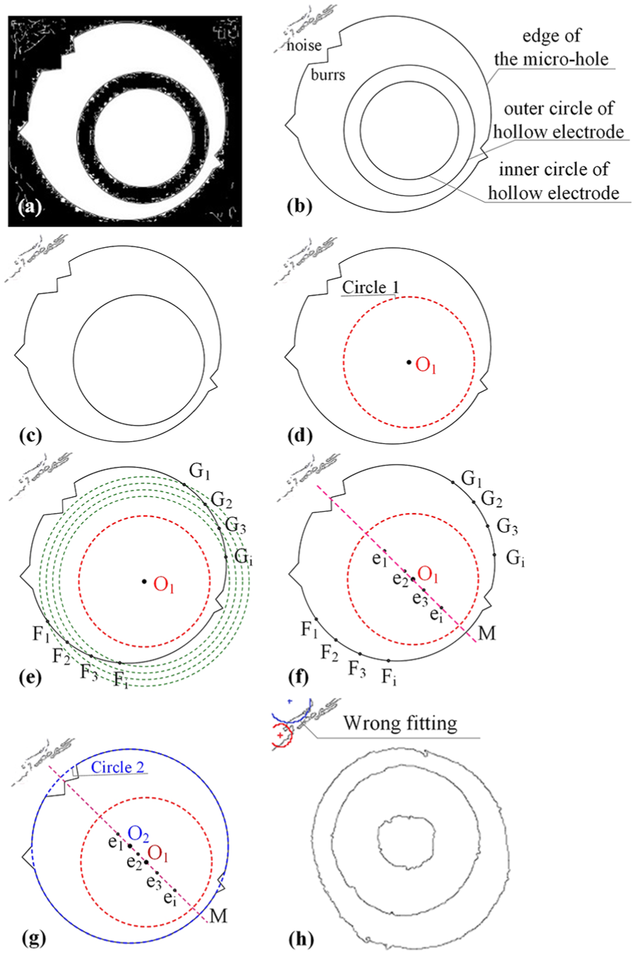
The non-standard nested circle-fitting process: (a) acquired image, (b) image preprocessing, (c) inner-circle filtering of the electrode, (d) outer-circle fitting of the hollow electrode, (e) intersected circle drawing, (f) intersection center calculation and center-constrained line drawing, (g) nested circle fitting, and (h) erroneous fitting.

It should be noted that the edge of the micro-hole is a non-standard circle. In order to improve the fitting accuracy, the sampling for equation (4) has to be conducted many times. A Gauss–Newton or Levenberg–Marquardt method ²² then has to be used to convert the least square with a linear constraint passing through the center to an unconstrained least square. Subsequently, the relevant parameters can be solved and the coordinates of center O₂ and radius R can be obtained, as shown in Figure 1(g). In the nested circle-fitting algorithm, the position of the circle center of the target circle (Circle 2) is limited by the linear constraint, thus avoiding the fitting result slipping away from the actual situation, as shown in Figure 1(h). By guaranteeing the fitting precision, the accuracy rate is also greatly improved.

Fitting experiments

Module setup for microscopic centering experiment

In order to verify the effectiveness of the nested circle-fitting algorithm based on the least-square method with a linear constraint passing through the center, a fitting comparison experiment was carried out using a bespoke microscopic centering device. The experiment setup is illustrated in Figure 2(a). It is mainly composed of a mechanical body, an image-acquisition module, a main control and display unit, a motion control driver, and a pulse power supply.

Figure 2.

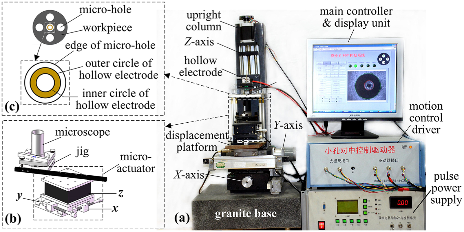
Microscopic centering experiment setup: (a) mechanical body, main control and display unit, motion control driver, and pulse power supply; (b) image-acquisition module; and (c) top view of the location relationship between the micro-holes and the hollow electrode during the centering process (nested circle formation).

The mechanical body had a vertical C-type structure, which was mainly made up of a granite base, an upright column, an X–Y displacement stage, a Z-axis movement mechanism, an electrode holder, and an electrolytic cell. The device had linkage feed from three axes. When combined with a precision motion servo-unit for the X, Y, and Z-axes, this setup was able to realize three-dimensional movement during centering and machining. The movement in each direction was controlled by a driver, a servomotor, a precision ball screw, and a grating ruler. The closed-loop system was controlled with a minimum feed resolution of 0.2 µm, ²³ which can achieve high-precision positioning and a stable low-speed feed.

In the experiment setup, the clamps of the tool electrode and the workpieces include a two-dimensional tilting mechanism and a left–right translation mechanism, respectively. By adjusting these mechanisms, the concentricity and the coaxially of the tool electrode may be ensured.

The image-acquisition module (Figure 2(b)) consisted of a micro-displacement actuator, a microscope, and a microscope jig. It was used to obtain a clear and complete image formed by the electrode and the workpiece, as shown in Figure 2(c), which contained a non-standard nested circle. The micro-displacement actuator had a resolution of 1 µm. It controlled the movement of the microscope in the X-, Y-, and Z-directions. The microscope had a numerical aperture of 0.05 and a resolution of 0.5 µm. The position of the microscope could be adjusted using the micro-displacement actuator in order to obtain a clear image. For the experimental module, the centering process was completed across the following steps: acquisition of a clear microscopic image, the fitting processing, and the position adjustment of the centering device.

Nested circle-fitting experiments

The nested circle-fitting experiments were carried out using the bespoke experimental module. The experimental process is shown in Figure 3. First of all, the original image was captured, as shown in Figure 3(a), with an image magnification of approximately 50. It can be seen from Figure 3(b) that, after binarization, some parts between the inner and outer circles of the electrode became black, with the circumference of the micro-holes becoming black as well. Alongside of this, a great deal of noise was observed. Applying the nested circle-fitting method based on the least-square method with a linear constraint passing through the center, the following post-processing steps were carried out: de-noising and edge extraction, electrode inner-circle filtering and outer-circle fitting, intersected circle and constrained line drawing, and micro-hole edge fitting. The results are shown in Figure 3(c)–(h).

Figure 3.

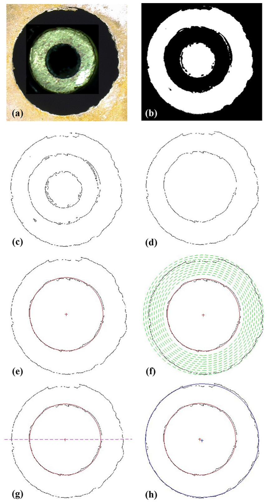
Fitting process for non-standard nested circles during the process of centering the micro-holes and the corresponding hollow electrode: (a) original acquired image, (b) binarization, (c) de-noising and edge extraction, (d) electrode inner-circle filtering, (e) electrode outer-circle fitting, (f) intersected circle drawing, (g) center-constrained line drawing, and (h) micro-hole edge fitting.

Analysis of the fitting results

Without changing the microscope position, magnification, and light intensity, the position of the electrode in the workpiece micro-hole was changed; 100 positions were arbitrarily selected, and three repeated images were collected at each position. Then, the least-square method with a linear constraint passing through the center (LSLC), the RCLS method, and the TLS method were each employed for fitting. The results were then compared and analyzed. Figure 4 shows the comparison results for the three fitting algorithms in terms of running time, memory usage, central processing unit (CPU) occupancy, and fitting accuracy. The experimental personal computer (PC) parameters were as follows: an Intel Core i7-7500 CPU (2.7 GHz, 2.8 GHz) and 8 GB of RAM.

Figure 4.

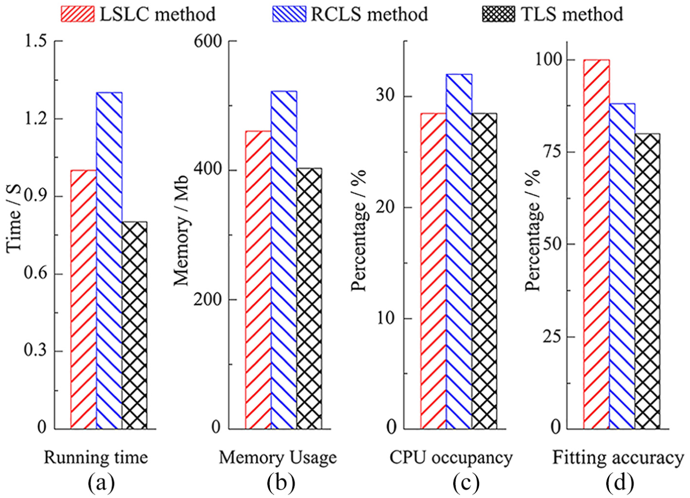
Performance comparison for the different fitting algorithms: (a) comparison of the running time, (b) comparison of memory usage, (c) comparison of CPU resource occupancy, and (d) comparison of fitting accuracy.

In terms of running time, the least-square method with a linear constraint passing through the center (LSLC) reduced the running time by 20% when compared to the RCLS method, but increased it by 15% when compared to the TLS method. In all cases, the running time was around 1 s. In terms of memory usage and CPU resource occupancy, the three fitting algorithms showed no significant difference. However, in terms of the accuracy of fitting, the least-square method with a linear constraint passing through the center was about 20% more accurate than the RCLS method. Most notably, it was about 30% more accurate than the TLS method, with an accuracy of over 99%.

Table 1 compares the typical fitting results for the LSLC, RCLS, and TLS methods. The TLS fitting results show two errors (third and ninth iterations). The RCLS fitting results show one error (seventh iteration), while the LSLC method produced no fitting errors in any of the 300 experiments.

Table 1.

Comparison of fitting results for RCLS, LSLC, and TLS.

Number of times	Algorithm	Mean value of fitting center coordinates/Pix	Mean value of fitting radius/Pix	Maximum deviation of fitting radius/Pix	Maximum deviation of fitting center/Pix	Is the fitting result correct?
1	RCLS	(278.71, 257.87)	201.77	−0.04	0.18	Yes
	LSLC	(278.77, 257.85)	201.73			Yes
	TLS	(278.64, 257.90)	201.81	+0.08	0.21	Yes
2	RCLS	(277.30, 253.41)	201.78	0.00	0.15	Yes
	LSLC	(277.86, 252.94)	201.78			Yes
	TLS	(277.86, 252.94)	202.79	+0.01	0.13	Yes
3	RCLS	(273.71, 251.32)	201.97	−0.08	0.15	Yes
	LSLC	(273.91, 251.59)	201.89			Yes
	TLS	(24, 170)	1.73	−202.03	263.89	No (Error)
4	RCLS	(275.79, 252.35)	201.93	−0.05	0.19	Yes
	LSLC	(275.82, 252.07)	201.88			Yes
	TLS	(275.84, 252.12)	201.95	+0.07	0.22	Yes
5	RCLS	(276.32, 252.92)	201.67	−0.01	0.11	Yes
	LSLC	(276.19, 252.02)	201.66			Yes
	TLS	(276.31, 252.13)	201.72	+0.06	0.19	Yes
6	RCLS	(276.32, 252.66)	201.81	+0.02	0.21	Yes
	LSLC	(276.45, 252.68)	201.83			Yes
	TLS	(276.51, 252.49)	201.89	+0.06	0.33	Yes
7	RCLS	(125.61, 90.88)	50.69	+150.7	214.05	No (Error)
	LSLC	(277.62, 251.88)	201.39			Yes
	TLS	(277.67, 251.99)	201.46	+0.07	0.15	Yes
8	RCLS	(277.51, 252.05)	201.18	+0.01	0.21	Yes
	LSLC	(277.31, 252.07)	201.19			Yes
	TLS	(277.43, 252.16)	201.27	+0.08	0.29	Yes
9	RCLS	(277.25, 251.24)	201.53	0.00	0.11	Yes
	LSLC	(277.41, 251.44)	201.53			Yes
	TLS	(3.1, 9.14)	2.13	200.41	369.01	No (Error)
10	RCLS	(277.56, 251.57)	201.56	0.00	0.26	Yes
	LSLC	(277.36, 251.72)	201.56			Yes
	TLS	(277.49, 251.75)	201.63	+0.07	0.14	Yes

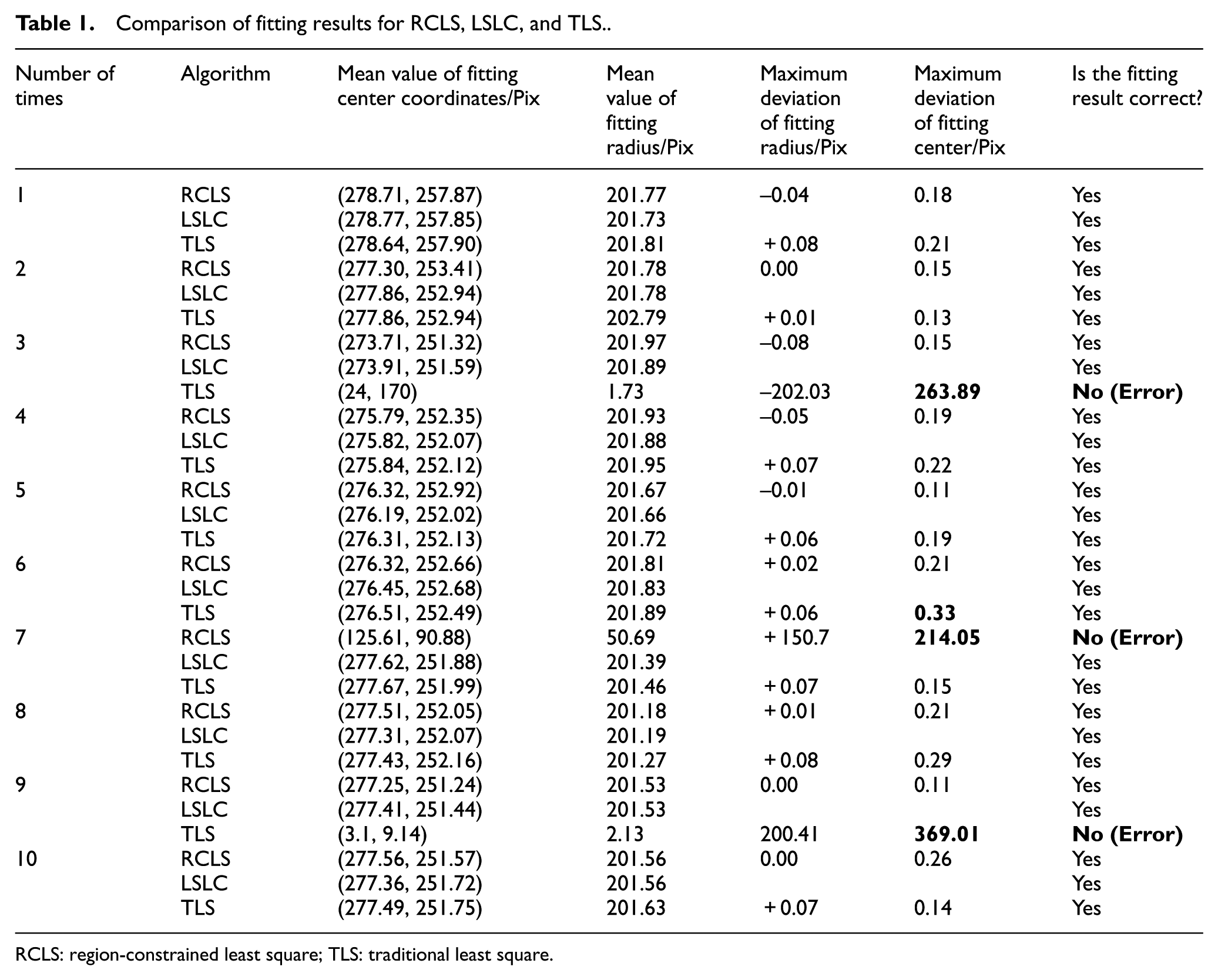
RCLS: region-constrained least square; TLS: traditional least square.

Figure 5(a) and (b) shows a comparison of the fitting results in terms of the radius and the center. The following conclusions can be drawn from Table 1 and Figure 5(a) and (b). (1) On the basis of the correct fitting results, the maximum deviation of the fitting radius was ±0.1 Pix (±0.5 µm) and the maximum deviation of the fitting center was ±0.33 Pix (±1.5 µm). Therefore, the least-square method with a linear constraint passing through the center and the RCLS method attained the same fitting precision as the TLS method. (2) The fitting results for the TLS method and the RCLS method sometimes produced an erroneous fitting. However, the fitting results for the least-square method with a linear constraint passing through the center were almost entirely correct, with an accuracy rate of over 99%.

Figure 5.

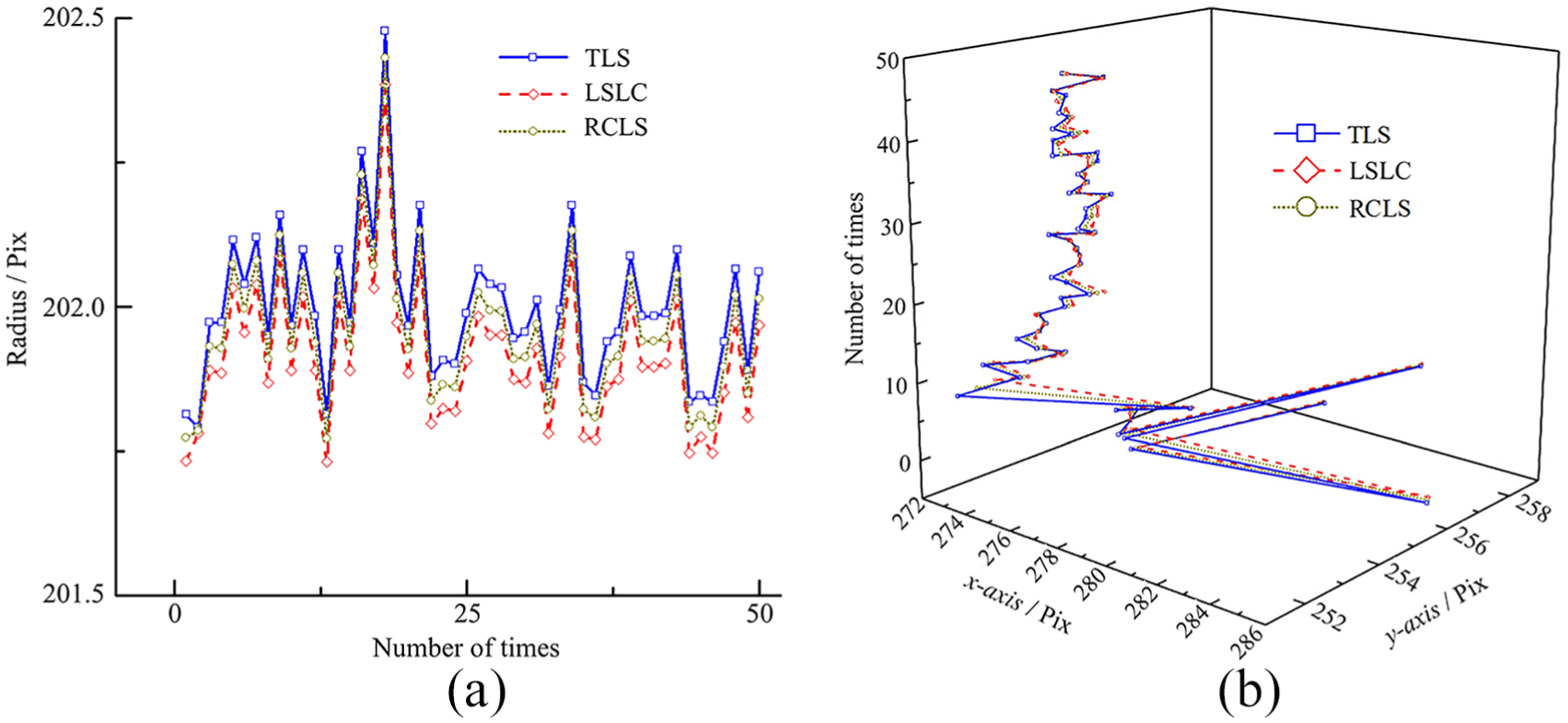
Comparison of fitting accuracy: (a) comparison of radius fittings (maximum deviation of fitting radius: ±0.1 Pix (±0.5 µm)) and (b) comparison of center points (maximum deviation of center from fitting center: ±0.33 Pix (±1.5 µm)).

The experimental results were also analyzed with regard to their algorithmic principles, bearing in mind that both the fitting method with a linear constraint passing through the center and the region-constrained method are directly derived from the TLS method. It can be seen, then, that the running time, processing complexity (i.e. memory usage, CPU occupancy), and fitting accuracy for the TLS method were poorer than the other two. However, the fitting precision of the three algorithms was basically the same. The region-constrained fitting method employs a chain-tracing structure by scanning the center region to constrain the position of the center. This helps to improve fitting accuracy to some extent. However, the big scanning region involves a large amount of computation, so the memory usage and CPU-occupancy rate are high and the process is more time-consuming. On top of this, the number of invalid cases cumulatively increases and the accuracy and performance quality drop off over time. The fitting method with a linear constraint passing through the center, however, by adopting a straight line through the center of the circle to be fitted as its constraint manages to improve the fitting accuracy while reducing the constrained region and computational burden. As a result, the memory usage, CPU-occupancy rate, and running time were all unexceptional in this case. We also found that all of our analysis results corresponded well with the experiments.

In conclusion, assuming the fitting results are correct, the fitting precision of the three algorithms is basically the same. However, when noise and burrs are present, the TLS method and the RCLS method may cause incorrect fitting results. As was seen in Figure 1(h), the electrode was mis-located during the secondary machining, which caused damage to the workpiece and the electrode. In this kind of case, the fitting algorithm for nested circles using the least-square method with a linear constraint passing through the center is the most optimal. On the premise that fitting precision and stability can be guaranteed, the accuracy can be greatly improved using this method. Thus far, then, the viability and validity of the algorithm has been verified.

Deburring process experiment

So far, we have seen that nested circle fitting using the least-square method with a linear constraint passing through the center can be applied to the centering process for micro-holes with a corresponding electrode. We now report on how an experimental study was carried out to explore its actual applicability to an electrochemical deburring process. The goal was to maintain the shape of the micro-hole and the dimensional precision and to assess whether the surface quality could be further improved. It also provided an opportunity to verify the feasibility of applying the method to an actual process.

Existing deburring methods are mainly mechanical and include abrasive grinding, thermal deburring, magnetic deburring, and electrochemical machining. ²⁴ Mechanical methods have the advantage of there being no residual stress on the deburred surface, no damage to the surface itself, and a low cost. However, these methods are not suitable for micro-holes with a diameter of between 0.1 and 1 mm. The abrasive grinding method generally wears the surface of the workpiece and enlarges the aperture. It is also difficult to wash the abraded fragments out of the micro-holes. Thermal deburring has a high machining cost. It can also cause secondary burrs and burns, and residual stress can be generated after the burrs have been removed. Magnetic deburring produces chamfers and counterbores. Electrochemical machining offers the highest deburring quality, a stable effect, high production efficiency, and a wide range of possible applications. This makes electrochemical machining the most effective approach for the deburring of metal alloy parts.

In order to ensure micro-hole shape precision and surface quality, we used the electrochemical machining method for our deburring process. As shown in Figure 6, the diameter D of the micro-hole was 0.5 mm. A hollow tube with an outer diameter Φ of 0.3 mm was selected as the electrode. The outer wall of the hollow electrode was covered with an insulating layer. The thickness of the insulating layer was 0.025 mm; h was defined as the distance between the insulating transparent baffle and the lower end of the hollow electrode (referred to as the machining gap).

Figure 6.

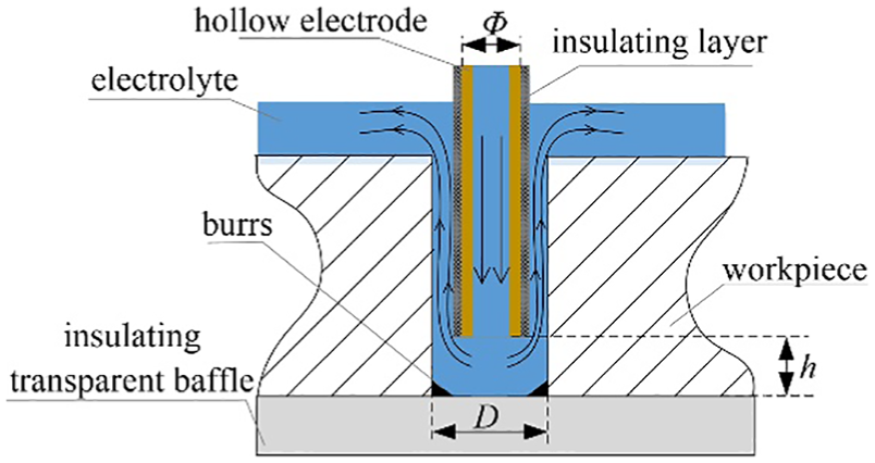
Electrolytic deburring process.

Considering the localization and efficiency together in micro-electrochemical machining, it is very important to select machining parameters. In our previous researches,^23,25 the multifactor and multivariate methods had been designed and validated, and the methods and machining parameters had been optimized by taking orthogonal experiments for differences in the process of machining. The results were as follows. First, for the sake of environmental considerations, a water-based neutral salt solution NaNO₃ was selected as the electrolyte for machining and then its concentrations were optimized. Second, the priorities of the other important parameters should be, first, machining voltage, and, second, pulse interval and pulse width, and feed speed and pressure have less effect on the method of electrochemical deburring in the given working condition.

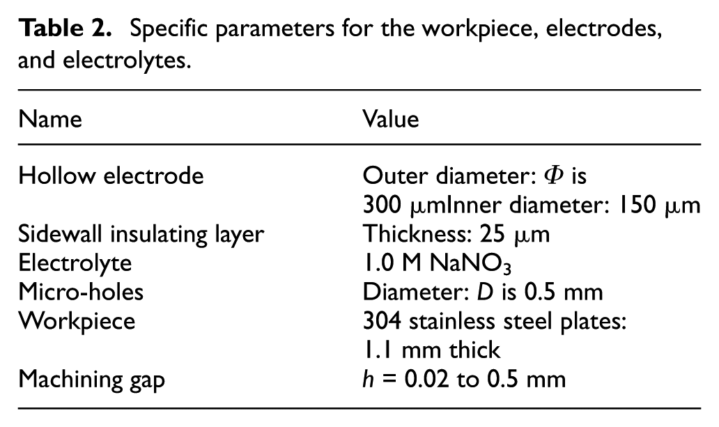
The workpiece material was a 304-stainless-steel flat plate with a thickness of 1.1 mm. Other specific parameters are shown in Table 2. Where there are constant electrode and machining gaps, optimal values can be determined for the machining parameters, such as the electrolyte concentration, the machining voltage, the pulse interval, and pulse width.

Table 2.

Specific parameters for the workpiece, electrodes, and electrolytes.

Name	Value
Hollow electrode	Outer diameter: Φ is 300 µmInner diameter: 150 µm
Sidewall insulating layer	Thickness: 25 µm
Electrolyte	1.0 M NaNO3
Micro-holes	Diameter: D is 0.5 mm
Workpiece	304 stainless steel plates: 1.1 mm thick
Machining gap	h = 0.02 to 0.5 mm

Electrolyte concentrations and machining voltage

Deburring effectiveness can be evaluated through the ratio of the amount of burr removal Δ to the enlargement of the micro-hole diameter Δϕ. This is called the removal-enlargement ratio and is denoted by K. It can be expressed as follows

$$K=\frac{\Delta }{\Delta \phi }$$

(5)

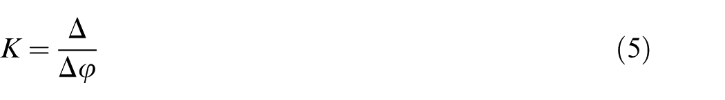
where the burr removal amount Δ denotes the average reduction in its radial length from the top of the burrs to the fitting edge of the machined micro-hole between before and after machining. It is better to have a larger burr removal amount Δ and a smaller enlargement size of micro-hole diameter Δϕ, which will thus increase the value of K. The deburring experiments reported here were carried out at concentrations of 0.5, 1.0, 1.5, 2.0, and 2.5 mol/L of the sodium nitrate electrolyte with a direct current (DC) voltage of 10 V. The effects of different machining currents and enlargement sizes of the micro-hole diameter are shown in Figure 7. Meanwhile, the value of the removal-enlargement ratio K was calculated and the results are shown in Figure 8. As the electrolyte concentration was increased, the machining current and enlargement size of the micro-hole diameter also increased. When the concentration was greater than 1.5 mol/L, the enlargement size of the micro-hole diameter was about 13 µm in 10 s of machining time, which is relatively large and does not meet the machining requirements (<10 µm). The overcut in the electrolytic deburring was greater; however, the burr removal amount Δ was basically unchanged. Therefore, the K value decreased with the increase of the concentration. It can be seen here that, when the concentration was between 0.5 and 1.5 mol/L, the value of K became quite large. When the concentration was 0.5 mol/L, the burr removal time became longer and the machining efficiency dropped, and the K value was also smaller after 10 s of machining time. When the concentration was about 1.0 mol/L, burrs were removed (the burr removal amount Δ was the maximum) and the enlargement size of the micro-hole diameter was about 8.5 µm in 10 s of machining time, which met the machining requirements (<10 µm) and the overcut in the electrolytic deburring was smaller. Therefore, the value of K value was at its largest (about 16.5) when the concentration was about 1.0 mol/L. This met the deburring efficiency requirement of a large amount of burr removal with a small enlargement in the size of the micro-hole diameter. All things considered, in that case, the most effective concentration of the electrolyte for deburring was selected to be at about 1.0 mol/L.

Figure 7.

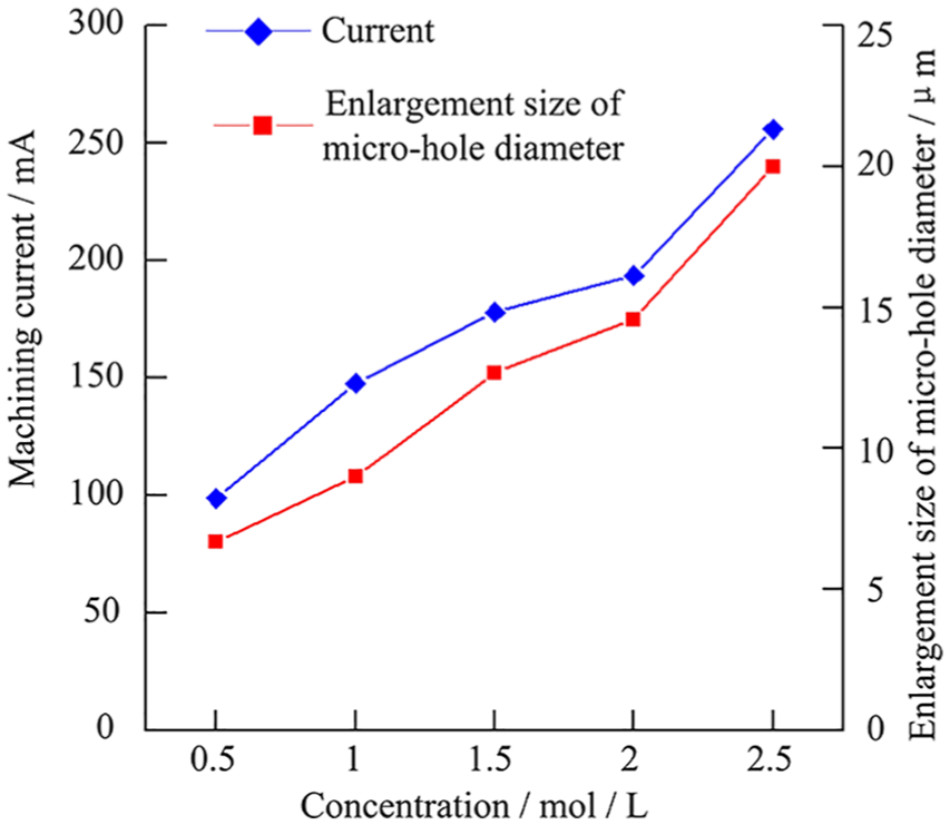
Machining current and hole enlargement size curves at electrolyte concentrations of 0.5, 1.0, 1.5, 2.0, and 2.5 mol/L with a machining voltage of DC 10 V and a machining time of10 s

Figure 8.

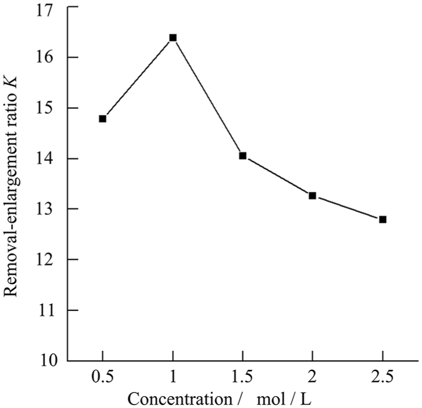
Removal-enlargement ratio K curve at concentrations of 0.5, 1.0, 1.5, 2.0, and 2.5 mol/L, with a machining voltage of DC 10 V and a machining time of 10 s.

Machining voltage is one of the key parameters. Once there is a specified electrolyte concentration, the machining voltage can be further optimized. We conducted deburring experiments at machining voltages of 5, 9, 13, and 15 V. The current and related enlargements of the micro-hole diameter at different voltages are shown in Figure 9. Machining was conducted at each voltage for a period of 10 s. It can be seen that the current increased gradually along with the increase in voltage. This means that the burr removal amount gradually increased as well. However, a large voltage also significantly increased the enlargement of the micro-hole diameter. At 5 and 9 V, the burrs left a large residue. However, while the burrs were completely removed at 15 V, the enlargement size was increased (to about 28 µm) and the edges of the burrs were found to be uneven. When the voltage was at 13 V, the removal-enlargement ratio K was approximately 15. At this point, the burr was basically removed, but the enlargement size was still relatively small (about 10 µm). This basically meets the machining requirements and can be further controlled through parameter optimization. The most effective machining voltage was therefore selected to be around 13 V.

Figure 9.

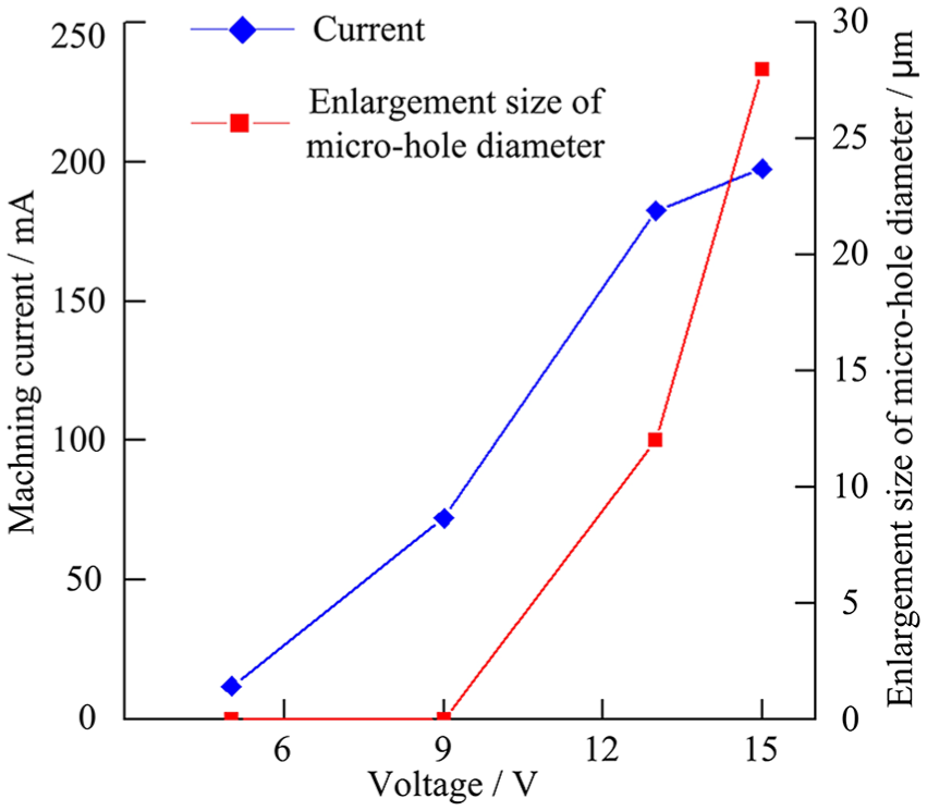
Changes in machining current and enlargement size of the micro-hole diameter at machining voltages of 5, 9, 13, and 15 V. In a 1.0 mol/L NaNO₃ electrolyte solution, when the machining voltage is 13 V, the burrs are basically removed and the hole enlargement size is about 10 µm, which meet machining requirements.

Pulse interval and pulse width

The shortest distance from the bottom burring in micro-holes to the electrode in the radial direction is about 20 ∼ 30 µm. Working on the basis of the principle of electrical double layering in electrochemistry ²⁶ and findings from previous experimental studies,^25,27,28 the overcut in the electrolytic deburring is controlled by the parameter of pulse interval and pulse width in this research. And the pulse interval and pulse width have an important effect on the localization in micro-electrochemical deburring. According to the above principles, the pulse interval was selected to be 100 µs and the pulse widths were selected to be 12, 25, 50, 75, and 100 µs. Burrs have an axial thickness of between 100 and 300 µm, and it is difficult to remove them completely with just a few seconds of machining. We therefore also designed a machining experiment that combined different pulse widths with different electrode positions (machining gap h). The pulse width T_on varied from 12 to 100 µs, and the machining gap h decreased from 0.2 to 0.1 mm. The experimental results are shown in Figure 10. Machining for 5 s at a machining gap h of 0.2 mm and a pulse width T_on = 75 µs, the removal-enlargement ratio K was as high as about 42. Large burrs were more or less removed and the hole enlargement size was small (<7 µm), which indicates a good burr removal effect. Machining for 5 s at a machining gap h of 0.1 mm with a pulse width T_on = 25 µs, the removal-enlargement ratio factor K was about 25 (which is still high) and small burrs were completely removed. The hole enlargement size was also small (<3 µm), and the end surface was smoother near the intersection line.

Figure 10.

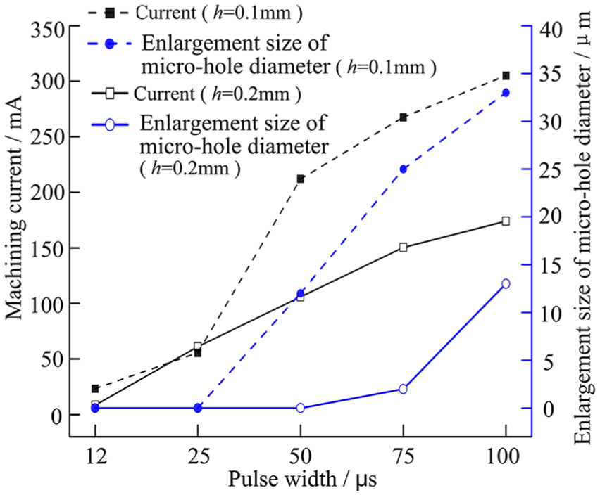
The relationship between the machining current and the hole enlargement size at different pulse widths (12, 25, 50, 75, and 100 µs).

When machining for a few seconds with a machining gap h of 0.2 mm and a large pulse width (75 µs), large burrs were basically removed and the hole was not enlarged (<3 µm). When processing for a few seconds with a small pulse width (25 µs) and a machining gap h of 0.1 mm, small burrs were removed and the hole was again not enlarged (<3 µm). In all of these experiments, the machining voltage was 13 V and the electrolyte was a 1.0 mol/L NaNO₃ aqueous solution.

Machining methods

With the overall goal of ensuring shape and dimensional precision, the deburring process was divided into two steps, rough and fine machining, which together sought to improve machining efficiency and surface quality. The specific steps were as follows.

1. Rough machining.

Here, the machining gap h was 0.2 mm and a large pulse width (75 µs) was used for the machining. This produced a large removal-enlargement ratio factor K of about 42 and large burrs were quickly removed, while the hole was not expanded and the expansion range remained less than 7 µm.

• 2. Fine machining.

Here, the machining gap h was 0.1 mm and a short pulse width (25 µs) was used for the machining. The removal-enlargement ratio value K was approximately 25, which was still high. Meanwhile, any residual burrs were completely removed. After the two machining operations, the enlargement size of the hole was still less than 10 µm overall.

The experimental results for the rough and fine deburring processes are shown in Figure 11. As can be seen in Figure 11(a), the maximum burr length before machining was 86 µm, and the micro-hole diameter was about 0.5 mm. After the rough machining, the large burr was more or less removed and the hole enlargement size was about 5 µm (see Figure 11(b)). After the fine machining (see Figure 11(c)), the burrs were completely removed. The enlargement size of the hole was approximately 3 µm. At this point, the shape of the hole was more rounded and the edges of the hole were clearer.

Figure 11.

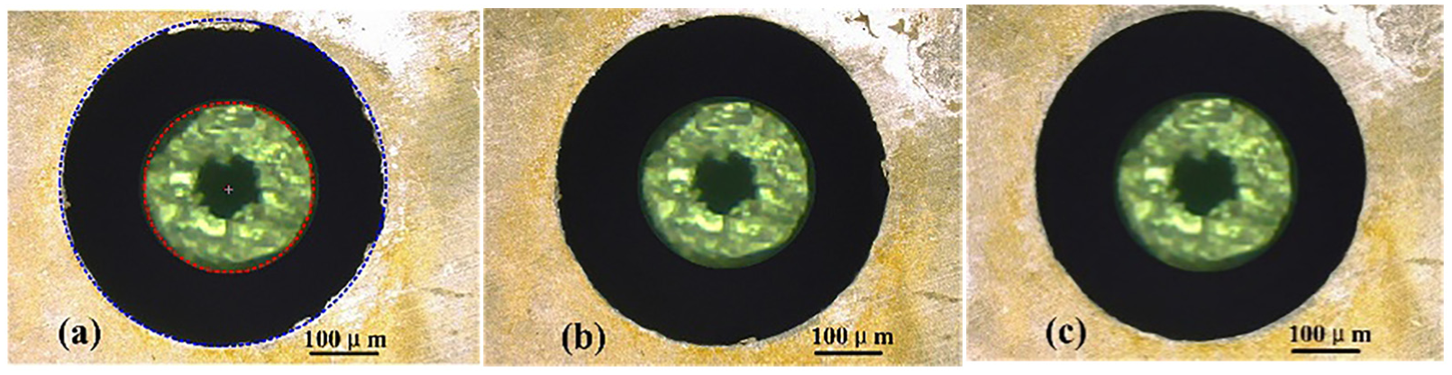
(a) The workpiece before deburring; (b) after rough machining, the large burrs have been basically removed and the hole diameter has increased by about 5 µm; and (c) after fine machining, the burrs have been completely removed and the hole enlargement size is about 3 µm.

After micro-EDM machining, the surface topography, roughness, and composition analysis were shown in Figure 12(a), (c), and (e). Figure 12(a) and (c) shows that the machined surface (the inner wall of the machined micro-hole) was covered with discharge pits; it was darker and there was a new white layer in some areas, and its surface topography poorer; and surface roughness, R_a, was about 1.2 µm. Figure 12(e) indicates that many tungsten (W) elements were present on the machined surface, except the main elements of the workpiece base material, such as ferrum (Fe), chrome (Cr), nickel (Ni), manganese (Mn), oxygen (O), and silicon (Si). This was because tungsten wire was used as the tool electrode for micro-EDM machining, so after the electrode had been dispersed through the spark discharge, many tungsten (W) elements remained in the recast layer on the machined surface.

Figure 12.

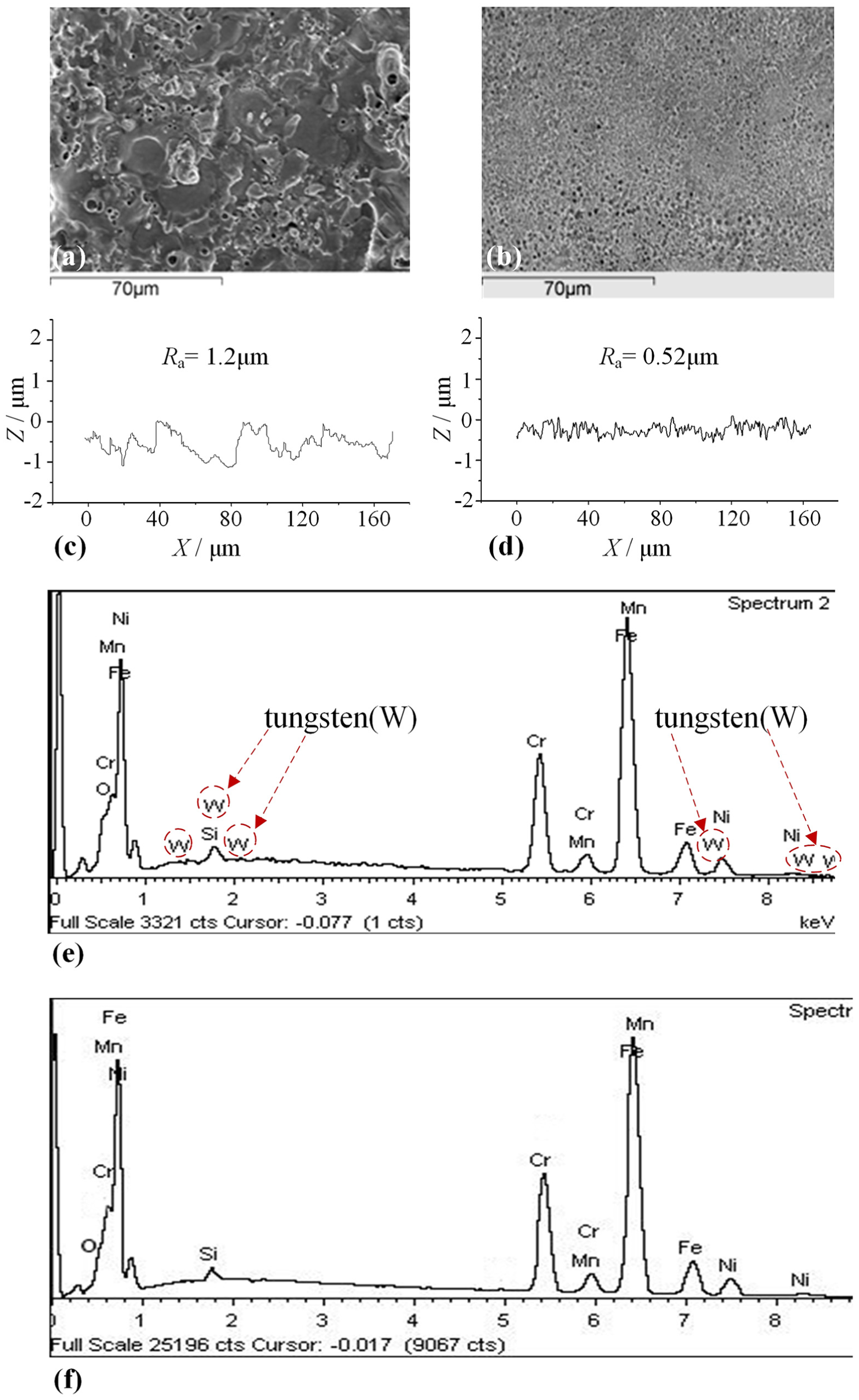
(a) After micro-EDM, the surface is covered with discharge pits; (c) the surface roughness R_a is about 1.2 µm; and (e) tungsten (W) is present on the machined surface. (b) After the electrochemical deburring process, the surface discharge pits are evidently smoother; (d) R_a is reduced to 0.52 µm; and (f) the tungsten (W) has been removed from the machined surface and the surface is back to being the workpiece base material, with the recast layer removed

The surface topography, roughness, and composition analysis after the secondary electrochemical deburring had taken place were shown in Figure 12(b), (d), and (f). Figure 12(b) and (d) shows that the surface discharge pits were evidently smoother, the white layer covered on the machined surface disappears, the machined surface became brighter, the surface topography better, and R_a was reduced to 0.52 µm. Figure 12(f) indicates that the tungsten (W) had been removed from the machined surface and the surface was back to being the workpiece base material, with the recast layer removed.

The above analysis of Figure 12 showed that, after the secondary electrochemical deburring process, the discharge pits on the machined surface were evidently smoother, the white layer disappeared, the surface became brighter, the roughness R_a had also reduced from 1.2 to 0.52 µm, and the surface had returned to the workpiece base material. Therefore, the affected recast layer had been removed. The two-step rough and fine machining method achieved full removal of burrs. So, in relation to the objective of ensuring shape and dimensional precision, the described process can be seen to improve both machining efficiency and surface quality.

Conclusion

To solve the problems (i.e. the accuracy rate and stability of the centering) of enabling secondary machining of micro-holes in metal alloy parts with a size of 0.1 ∼ 1 mm, a non-standard nested circle-fitting method based on the least-square method, with a linear constraint passing through the center, was developed and implemented in this article. The results showed that the proposed circle-fitting method attained the same fitting precision, compared to other existing approaches. At the same time, the accuracy rate was increased by at least 20%, delivering a result of more than 99%, so the accuracy of the fitting and the stability of the centering were significantly improved.

The above nested circle-fitting method was implemented in an experimental electrochemical deburring study. With the overall goal of ensuring centering, a rough-and-fine deburring process had been explored. The combined two-step deburring process ensured the precision of the shape and size, and effectively improved the machining efficiency and surface quality. In addition, the experiment provided concrete validation of the feasibility of the nested circle-fitting method we have proposed.