Sage Journals: Discover world-class research

Abstract

Because micro-line segments are the most widely used form of tool-paths for computer numerical control machining, the smoothness at the junction of two adjacent segments is still the bottleneck for the machining quality and efficiency. To reduce the time spent by the smoothing process and improve the smoothness at the junction, this article proposes a real-time and look-ahead interpolation algorithm with an axial jerk-smooth transition scheme. In one step, the algorithm finishes the transition scheme construction and velocity planning by using the trigonometric velocity planning method. This method can utilize the maximal acceleration and/or jerk capabilities of drive axis to achieve smooth axial kinematic profiles while satisfying the user-specified chord error. In addition, a real-time look-ahead method is developed to plan the global feedrate profile and adjust the transition schemes without intersections constantly. The simulation results demonstrate that the proposed algorithm could realize smooth axial velocity, acceleration and jerk control and improve the smoothing process efficiency and machining accuracy.

Keywords

Real-time look-ahead axial jerk-smooth transition scheme trigonometric velocity planning method computer numerical control micro-line segments

Introduction

For the computer numerical control (CNC) machining of complex curves and surfaces such as impellers, blades and aerospace components, short line segments or G01 codes are still the most widely used form of tool-paths. If linear paths are interpolated directly, discontinuities of velocities at junctions of adjacent segments will bring about large fluctuations of velocity, acceleration and jerk of drive axis,¹ which causes vibrations of the machine tool and reduces the machining efficiency and quality. Therefore, a significant amount of research has been conducted to obtain smooth trajectories, including the global smooth method (GSM) and local smooth method (LSM).

In the GSM method, tool-paths that comprise micro-line segments are transformed into one or several smooth spline curves by an approximation or interpolation approach. For example, FANUC and SIEMENS companies proposed the Smooth Tolerance⁺ Control function² and Advanced Surface and Top Surface function,³ respectively, which generate a smooth curve for a machining path specified with continuous small blocks. The methods used in these approaches are, however, not available in the published literature. Zhang et al.^4,5 adopted the cubic spline curve to interpolate tool-paths, which can pass exactly through all the data points. Zhang et al.⁶ extended the cubic spline curve to the quintic polynomial curve with the least-square method. Another method is based on the Akima spline curve,^7,8 in which the curve not only passes through all the data points exactly but also has the first-derivative continuity. However, these three kinds of spline curves are locally defined, therefore any change in one data point can significantly affect several adjacent points. Hence, many researchers have focused on the use of B spline curve.^9–11 Yang et al.¹² fitted polyline machining tool-paths into quadratic B spline curves with respect to time parameter. In order to reduce the number of control points and iterations, Zhao et al.¹³ found dominant points from discrete data points and approximated them into cubic B spline curves, but only the G0 continuity was achieved at the junction of adjacent curves. Zhao et al.¹⁴ constructed G2 continuous Bézier curves without iterations, but only the second-order Taylor expansion formula was used to estimate and control fitting errors. Wang and Yau¹⁵ developed a real-time NURBS interpolation methodology with a look-ahead function to recognize line segments which could be transformed into continuous NURBS blocks. Although the GSM could achieve very smooth trajectories that approximate the original curves closely, the method presents the following three shortcomings. First, the complex fitting conditions lead to heavy computation load with the required iterative algorithms. Second, it is difficult to calculate fitting errors accurately, and the process of adjusting the parametric curves is complicated. Third, inevitable errors caused by utilizing truncated Taylor series result in fluctuations in the feedrate.

For the LSM, tool-paths are blended by inserting curves, such as arcs or parametric curves, in junctions of adjacent short line segments to improve velocity profile while passing through the corners. Because these processes are local and contour errors can be easily controlled, many researchers have focused on this method. Lee and Hascoet,¹⁶ Zhang and Zhou¹⁷ and Lv et al.¹⁸ constructed a circular arc tangent to adjacent line sections at the corners. Zhang et al.¹⁹ adopted the quintic polynomial curve, and Ernesto and Farouki²⁰ utilized the rational quadratic Bézier curve. But these methods only provide velocity continuity or G1 continuity at the junctions, which would result in normal acceleration-induced vibration. Hence, Sencer et al.²¹ fitted quintic B spline curves to smooth the blocks, which ensures continuous curvatures or G2 continuity. Du et al.²² adopted the cubic Bézier curve, but the method needs a significant amount of calculation to estimate the proper transition lengths. Yutkowitz and Chester²³ realized corner-blending with two fourth-order polynomial curves at the cost of significant computational load. Zhao et al.²⁴ achieved curvature-continuous trajectories by inserting two symmetric cubic B Splines in the junction. In order to further improve the continuity, Fan et al.²⁵ generated curvature-smooth or G3 continuous tool-paths with two quartic Bézier curves, which is helpful to reduce vibration in machinery. However, even though the reviewed algorithms can obtain smooth trajectories and motion profiles, they still have the following three basic drawbacks. First, they need two computational steps. In the first step, the transition geometry is constructed by inserting parametric curves at the corners. In the second step, according to synthesized trajectories, the motion profiles are scheduled. This method is therefore not very efficient. Second, it is difficult to calculate the curve lengths accurately. Third, by only considering tangential kinematic limits, fluctuations are caused in the velocity, acceleration and/or jerk in the drive axis direction. Recently, the one-step LSM, in which the transition curve construction and velocity planning are conducted in one step, has attracted the interest of researchers. Sencer et al.²⁶ and Biagiotti and Melchiorri²⁷ adopted finite impulse filters to smooth linear paths, but the method causes unavoidable delay and large contour errors. Zhang et al.²⁸ utilized the quadratic Bézier curve in the time domain and axial linear acceleration and deceleration approach to achieve optimal interpolation, but the method does not guarantee chord error and axial jerk bounds.

Tsai and Huang²⁹ incorporated servo dynamics into transition curve generation to improve dynamic contour accuracy. Duan and Okwudire³⁰ used optimal control to generate time-optimal kinematic trajectories. However, these one-step algorithms only consider axial acceleration limit. Tajima and Sencer³¹ developed a kinematic corner smoothing algorithm based on a jerk-limited acceleration profile to achieve optimal-time feed motion. The method, however, assumes that G01 blocks are long enough so that corners could be blended without interfering with adjacent transition curves. In addition, changes in jerk can occur at the corners since a jerk-limited acceleration method is used.

In this article, a real-time and look-ahead interpolation algorithm with an axial jerk-smooth transition scheme is proposed for CNC machining of micro-line segments, which would improve the efficiency of the smoothing process and the resulting smoothness. In section “Transition scheme,” the proposed algorithm is used to construct transition curves and conduct velocity scheduling in one step using the trigonometric velocity planning method (TVPM). TVPM can utilize the maximal acceleration and/or jerk capabilities of the drive axis to achieve smooth axial kinematic profiles while satisfying the user-specified chord error. In section “Real-time interpolation with look-ahead function,” a real-time look-ahead model is developed for planning the global feedrate profile to guarantee attainment of two corner velocities on every block. In section “Simulation validations,” simulation results validating the proposed approach are presented. Concluding remarks are provided in section “Conclusion and discussions.”

Transition scheme

Transition curves are constructed by planning motion profiles of the axes, which is different from the traditional LSM, in which parametric curve fitting is followed by tangential feedrate scheduling. In this section, a scheme is presented for synthesizing the transition under chord error and axial kinematic constraints to achieve axial jerk-smooth motion profiles.

Trigonometric velocity planning method

In contrast to jerk-limited velocity planning methods, TVPM can achieve a jerk-smooth profile without exhibiting sudden changes in jerk at the corners. Supposed that the initial and terminal acceleration and jerk are zero and that the velocity increases from v_s to v_e during the period T. The trigonometric displacement function can then be described as follows

s (t) = a + bt + c t^{2} + d \cos (et)

(1)

where t denotes the time, $t \in [0, T]$ ; a, b, c, d and e are constant coefficients.

Taking the first, second and third derivatives of equation (1) with respect to the time, the velocity, acceleration and jerk functions are obtained as follows

v (t) = b + 2 ct - de \sin (et)

(2)

a (t) = 2 c - d e^{2} \cos (et)

(3)

j (t) = d e^{3} \sin (et)

(4)

Figure 1 shows the jerk-smooth motion profiles. Here, for the given initial and terminal conditions, the following relationships are derived for the time t = 0 and t = T

s (0) = a + d = 0

(5)

v (0) = b = v_{s}

(6)

a (0) = 2 c - d e^{2} = 0

(7)

a (T) = 2 c - d e^{2} \cos (eT) = 0

(8)

j (0) = 0 = 0

(9)

j (T) = d e^{3} \sin (eT) = 0

(10)

Figure 1.

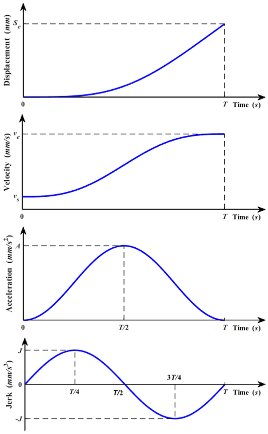
Jerk-smooth motion profiles.

Let J and –J indicate the maximum and minimum jerk, respectively, and the maximum acceleration be A. Then as shown in Figure 1, the acceleration curve reaches its maximum at the time t = T/2. Then from equation (3)

a (T / 2) = 2 c - d e^{2} \cos (eT / 2) = A

(11)

And the jerk curve achieves the maximum and minimum at the times t = T/4 and t = 3T/4, respectively, as follows

j (T / 4) = d e^{3} \sin (eT / 4) = J

(12)

j (3 T / 4) = d e^{3} \sin (3 eT / 4) = - J

(13)

To simplify coefficient calculations, let

eT = 2 π

(14)

Then, from equations (5) to (14), the coefficients are calculated as follows

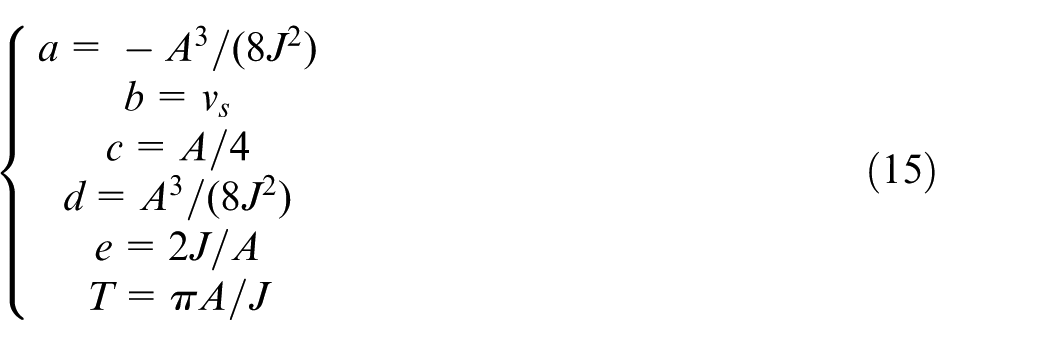
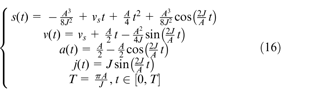
{\begin{matrix} a = - A^{3} / (8 J^{2}) \\ b = v_{s} \\ c = A / 4 \\ d = A^{3} / (8 J^{2}) \\ e = 2 J / A \\ T = π A / J \end{matrix}

(15)

Finally, the jerk-smooth kinematic functions are obtained as given in equation (16) by substituting the coefficient equation (15) into equations (1)–(4)

{\begin{matrix} s (t) = - \frac{A^{3}}{8 J^{2}} + v_{s} t + \frac{A}{4} t^{2} + \frac{A^{3}}{8 J^{2}} \cos (\frac{2 J}{A} t) \\ v (t) = v_{s} + \frac{A}{2} t - \frac{A^{2}}{4 J} \sin (\frac{2 J}{A} t) \\ a (t) = \frac{A}{2} - \frac{A}{2} \cos (\frac{2 J}{A} t) \\ j (t) = J \sin (\frac{2 J}{A} t) \\ T = \frac{π A}{J}, t \in [0, T] \end{matrix}

(16)

Transition construction scheme with prescribed chord error and axial jerk-smooth motion profiles

The proposed transition scheme is illustrated in Figure 2. The point P_s,i is chosen as the origin to establish the x–y coordinate system. The corner consists of two line segments P_i_–1P_i and P_iP_i₊₁ with lengths l_i and l_i₊₁, respectively. The curve with dotted line from the point P_s,i to the point P_e,i is the synthesized transition curve with the corner length L_c,i for the line segments P_s,iP_i and P_iP_e,i. In order to reduce the transition construction complexity, we let the lines P_s,iP_i and P_iP_e,i to be equal in length and assume that the corner motion has equal initial and terminal tangent velocity v_c,i, acceleration a_c,i = 0 and jerk j_c,i = 0. Hence, the objective of this section is to determine the maximum corner velocity v_c,i and length L_c,i based on a prescribed chord error $ε$ and axial TVPM.

Figure 2.

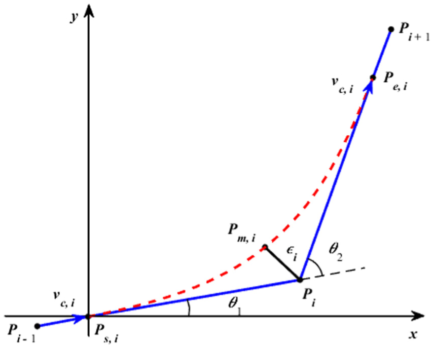
Transition construction scheme.

To find the maximum corner velocity v_c,i, at least one of the axis acceleration or jerk limit must be saturated. Hence, v_c,i should be determined by the axis experiencing the largest velocity change at the corner, namely, the limiting axis.

As an example, let the x-axis be the limiting axis, and let A_x and J_x indicate the acceleration and jerk of the x-axis; A_x_max and J_x_max indicate their limits, respectively; and F indicates the programmed feedrate. In this example, three constraints, namely, the peak acceleration and jerk in the x-axis are limited to A_x_max and J_x_max, respectively, and the contour error ε_i, Figure 2, is bounded.

First, the boundary velocities should be bounded. From Figure 2, the start and end velocities of x-axis are defined as follows

v_{sx, i} = v_{c, i} \cos θ_{1}

(17)

v_{ex, i} = v_{c, i} \cos (θ_{1} + θ_{2})

(18)

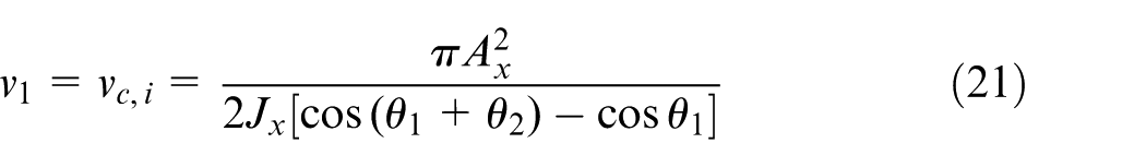
where θ₁ is the angle between the vector P _i–1 P _i and the positive x-axis and θ₂ is the angle between the vectors P _i–1 P _i and P _i P _i+1.

From equation (16) at the time t = T, we get the end velocity as follows

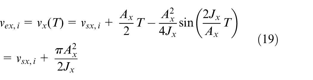
\begin{matrix} v_{ex, i} = v_{x} (T) = v_{sx, i} + \frac{A_{x}}{2} T - \frac{A_{x}^{2}}{4 J_{x}} \sin (\frac{2 J_{x}}{A_{x}} T) \\ = v_{sx, i} + \frac{π A_{x}^{2}}{2 J_{x}} \end{matrix}

(19)

Substituting equations (17) and (18) into equation (19), we can get

v_{c, i} \cos (θ_{1} + θ_{2}) = v_{c, i} \cos θ_{1} + \frac{π A_{x}^{2}}{2 J_{x}}

(20)

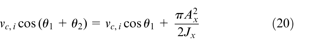
Then by adjusting equation (20), the corner velocity v₁ is achieved as follows

v_{1} = v_{c, i} = \frac{π A_{x}^{2}}{2 J_{x} [\cos (θ_{1} + θ_{2}) - \cos θ_{1}]}

(21)

Second, to avoid intersection of adjacent transition curves, the corner motion length L_c,i is constrained to

L_{c, i} = min (l_{i} - L_{c, i - 1}, l_{i + 1} / 2)

(22)

where L_c,i–1 is the corner length of the previous corner $∠ P_{i - 2} P_{i - 1} P_{i}$ .

The x-axis displacement s_cx,i is calculated based on the corner geometry as follows

s_{cx, i} = L_{c, i} \cos θ_{1} + L_{c, i} \cos (θ_{1} + θ_{2})

(23)

From equation (16) at the time t = T, we can also get the displacement s_cx,i as follows

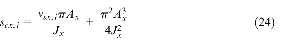
s_{cx, i} = \frac{v_{sx, i} π A_{x}}{J_{x}} + \frac{π^{2} A_{x}^{3}}{4 J_{x}^{2}}

(24)

Then from the equations (17) and (22)–(24), the corner velocity v₂ becomes

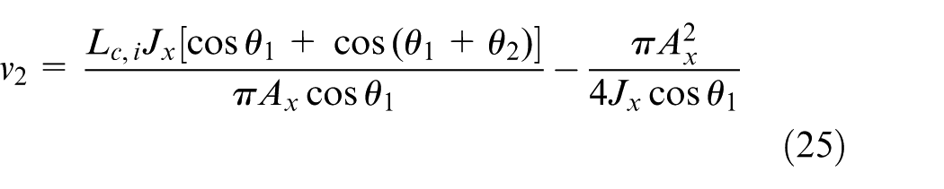
v_{2} = \frac{L_{c, i} J_{x} [\cos θ_{1} + \cos (θ_{1} + θ_{2})]}{π A_{x} \cos θ_{1}} - \frac{π A_{x}^{2}}{4 J_{x} \cos θ_{1}}

(25)

Third, the chord error is also considered to be bounded. As can be seen in Figure 2, P_m,i is the mid-point of the transition curve. Since the initial and terminal tangent velocities, accelerations and jerks of the corner motion are the same, the transition curve is symmetric about the bisector of the angle $∠ P_{i - 1} P_{i} P_{i + 1}$ , and the maximum contour error ε_i is the distance between the points P_i and P_m,i.

The x-coordinate of the point P_i is seen in Figure 2 to be

x_{i} = L_{c, i} \cos θ_{1}

(26)

The projection of corner error ε_i on the x-axis is also seen to be

ε_{x, i} = ε_{i} \cos (\frac{π}{2} + θ_{1} + \frac{θ_{2}}{2})

(27)

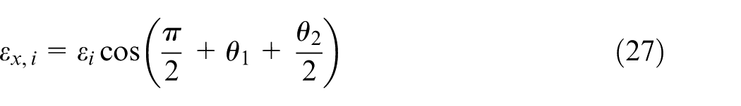
From equation (16), the x coordinate of the point at the time t = T/2 is as follows

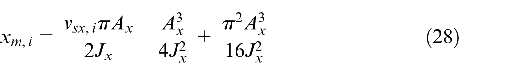
x_{m, i} = \frac{v_{sx, i} π A_{x}}{2 J_{x}} - \frac{A_{x}^{3}}{4 J_{x}^{2}} + \frac{π^{2} A_{x}^{3}}{16 J_{x}^{2}}

(28)

Now let x_m,i – x_i =ε_x,i and ε_i = ε. Then the corner velocity v₃ is calculated from equations (17) and (26)–(28) as follows

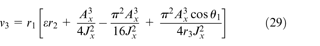
v_{3} = r_{1} [ε r_{2} + \frac{A_{x}^{3}}{4 J_{x}^{2}} - \frac{π^{2} A_{x}^{3}}{16 J_{x}^{2}} + \frac{π^{2} A_{x}^{3} \cos θ_{1}}{4 r_{3} J_{x}^{2}}]

(29)

where

\begin{matrix} r_{1} = \frac{2 r_{3} J_{x}}{π A_{x} \cos θ_{1} [\cos (θ_{1} + θ_{2}) - \cos θ_{1}]} \\ r_{2} = \cos (\frac{π}{2} + θ_{1} + \frac{θ_{2}}{2}) \\ r_{3} = \cos θ_{1} + \cos (θ_{1} + θ_{2}) \end{matrix}

Finally, the maximum corner velocity v_c,i is determined by the programmed limitation on the feedrate and bounds on the velocity, corner length and chord error, that is

v_{c, i} = min (F, v_{1}, v_{2}, v_{3})

(30)

Now the initial and terminal velocities v_sx,i and v_ex,i are given by equations (17) and (18), respectively. A_x is computed by substituting v_c,i and J_x =J_x_max into equation (21). And L_c,i is achieved from equation (25) with v₂ = v_c,i, A_x and J_x. We can then determine the desired jerk-smooth trajectory for the x-axis by substituting the calculated values into equation (16). Then, let the y-axis be the limiting axis, and the jerk-smooth trajectory for y-axis is synthesized using the same process with similarly applicable operational limitations for the axis.

If T_y > T_x, y is the real limiting axis. In order to synchronize the corner motion, we need to adjust A_x, J_x according to equations (16) and (19) with the motion period of y-axis T_y for re-synthesizing the jerk-smooth trajectory of x-axis; Otherwise, x is the real limiting axis. Similarly, the jerk-smooth trajectory of y-axis is re-created with T_x, recalculated A_y and J_y.

Real-time interpolation with look-ahead function

Figure 3 illustrates the flow chart of the present real-time interpolation scheme with the look-ahead characteristic feature. It can be seen that the look-ahead scheme process involves two modules: the initialization module, which is used to construct smooth trajectories and axial motion profiles without the intersection of adjacent transition curves and the backward scanning module, which guarantees the global feedrate profile and accessibility of corner velocities. These two modules are described in the following sections.

Figure 3.

Flow chart of real-time interpolation with look-ahead function.

Look-ahead initialization

A look-ahead buffer with N units is used to store the kinematic information of line segments and transition curves as shown in Figure 4. Before machining, the N line segment data loaded into the buffer and the transition schemes are constructed as was described in section “Transition scheme.” Then, trajectories comprising line segments and transition curves are obtained as shown in Figure 5. L_i and L_i₊₁ are corner lengths of joint points P_i and P_i₊₁, and v_c,i and v_c,i+1 are their corner velocities, respectively. l_i₊₁ is the length of the i + 1th line segment, and d_i₊₁ is its interpolation length.

Figure 4.

Look-ahead buffer.

Figure 5.

Synthesized trajectories.

Backward scanning

To guarantee that on every line segment the tangential velocity can change from v_c,i to v_c,i+1 within the length d_i₊₁ and that the global velocity profile can be achieved, the following five steps are needed to be executed in this module:

Step 1. Let the start velocity of the first segment v_c,0 and the end velocity of the Nth segment v_c,N be equal to zero in the buffer, and let j = N – 1, p = 0.

Step 2. Use the TVPM to plan motion profiles from v_c,j+1 to v_c,j along the interpolation length d_j₊₁.

If the planning succeeds, the terminal condition is satisfied. Otherwise, perform the following process to reduce the velocity v_c,j or v_c,j+1:

If v_c,j < v_c,j+1, calculate the maximum reachable velocity $v'_{c, j + 1}$ , from which the speed decelerates to v_c,j, let $v_{c, j + 1} = v'_{c, j + 1}$ and j = j + 1 and reconstruct the transition scheme. Then return to Step 2. Otherwise, compute the maximum $v'_{c, j}$ , to which the speed accelerates from v_c,j+1.

Step 3. The backward scanning process is finished only when one of the following two conditions is satisfied:

j ≤ 0.

p = 1 and the terminal condition is satisfied.

Otherwise, let $v_{c, j} = v'_{c, j}$ and reconstruct the transition scheme. Then, set j = j – 1 and return to Step 2.

Step 4. Real-time interpolation: Take the first segment to machine. When finished, delete it from the buffer. If p equals to zero, set p = 1.

Step 5. Add a new line segment at the end of the buffer, set its end velocity equal to zero and construct the transition scheme. Then let j = N – 1 and go to Step 2 to do the backward scanning process again.

Simulation validations

In this section, the results of simulations that are performed to validate the feasibility, effectiveness and performance of the proposed real-time look-ahead interpolation algorithm with axial smooth transition scheme are presented.

Case 1

In this simulation, the proposed algorithms are implemented with VS2013, and the software used for plotting is MATLAB 2015. For the hardware, Intel Atom N450 CPU 1.66GHz is used. As shown in Figure 6(a), the lightning-shaped tool-paths with two obtuse angles is utilized. The machining direction starts from point B and ends at point E. The tangential federate F is set to 50 mm/s, the acceleration and jerk limits for both axes are considered to be A_x_max =A_y_max = 2000 mm/s² and, J_x_max =J_y_max = 250,000 mm/s³, respectively. The sample time and chord error limit are considered to be T = 0.002 s and ε = 0.1 mm, respectively.

Figure 6.

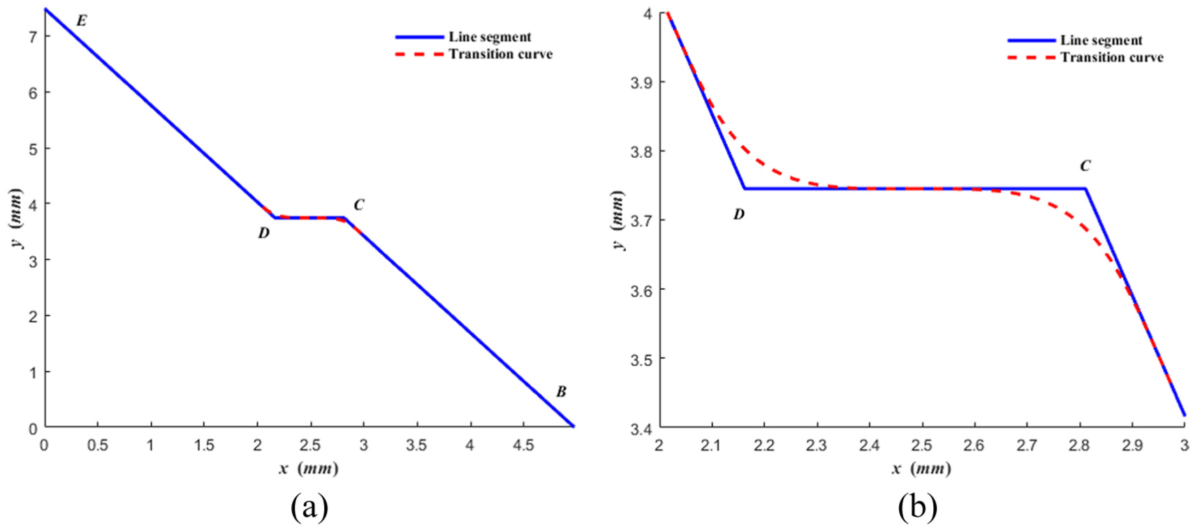
Tool-paths of case “1”: (a) synthesized trajectories and (b) enlarged profile of corners C and D.

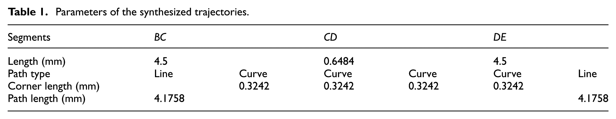
After applying the smoothing algorithm, the synthesized trajectories comprising line blocks and curves are presented in Figure 6(a). To illustrate the transition scheme clearly, profiles of the corners C and D are enlarged, as shown in Figure 6(b). From Figure 6(b), we can see that these two curves do not overlap. In Table 1, corner lengths of angles $∠ BCD$ and $∠ CDE$ are both 0.3242 mm, which is half the length of segment CD. Therefore, the proposed algorithm can avoid the intersection of adjacent transition curves.

Table 1.

Parameters of the synthesized trajectories.

Segments	BC		CD		DE
Length (mm)	4.5		0.6484		4.5
Path type	Line	Curve	Curve	Curve	Curve	Line
Corner length (mm)		0.3242	0.3242	0.3242	0.3242
Path length (mm)	4.1758					4.1758

The simulation results are shown in Figure 7. Figure 7(c) shows the resulting jerk profiles for the x-axis and y-axis jerk curves. It can be seen that the jerks do not exceed the specified limits amounts and that they are both smooth and without sudden changes at corners. The acceleration and velocity profiles are shown in Figure 7(a) and (b), respectively. The contour error curve is shown in Figure 7(d) and is seen to stay within the specified limit of ε. It is therefore concluded that the proposed algorithm would yield trajectories that satisfy the specified requirements and drive constraints for machining accuracy

Figure 7.

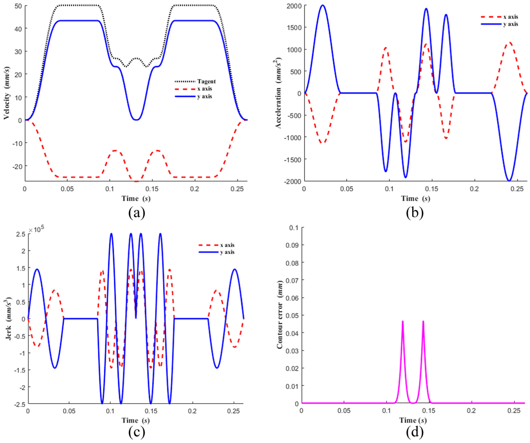
Simulation results of the case “1”: (a) velocity, (b) acceleration, (c) jerk and (d) contour error profiles.

Case 2

To evaluate the proposed algorithm, the following two algorithms were also implemented as the basis for comparison: a jerk-limited algorithm³¹ and a polynomial algorithm.¹⁹ The jerk-limited algorithm³¹ achieves the transition curve and axial jerk-limited motion profiles in time domain in one step. The polynomial algorithm¹⁹ uses the quintic polynomial to construct the transition curve in arc length domain and then uses a trigonometric velocity planning method to schedule the blended tool-paths.

The proposed algorithm obtains the transition curve and axial jerk-smooth motion profiles in time domain in one step as described in section “Real-time interpolation with look-ahead function.”

The jerk-limited algorithm³¹ is selected as one of the comparison algorithms since this algorithm can obtain axial jerk-limited profiles, while other one-step algorithms^26–30 only consider the axial acceleration limits. In addition, the jerk-limited and the proposed algorithms both use velocity planning to synthesize transition curves. Meanwhile, to show the difference between one-step and two-step methods, the quintic polynomial algorithm¹⁹ is used as the comparison algorithm. In this method, the transition curve construction and the kinematic scheduling are separately implemented, and the conventional trigonometric velocity planning method is employed to schedule the blended toolpath.

To validate the effectiveness of the proposed method, the smoothness and the required computing times of the synthesized motion trajectories are utilized as the evaluation indexes.

In this case, the following typical settings are considered: a tangential feedrate of F = 100 mm/s, acceleration limit of the drive axes A_x_max=A_y_max=2000 mm/s², jerk limit of the drive axes J_x_max=J_y_max=100,000mm/s³, a sample time of T = 0.002 s and a chord error limit of ε = 0.1 mm.

The trident-shaped pattern, Figure 8, is employed as the tool-paths. It consists of two acute angles, one right angle and two obtuse angles. After the smoothing processing of the three algorithms, the synthesized trajectories and enlarged corner transition curves are shown in Figure 8.

Figure 8.

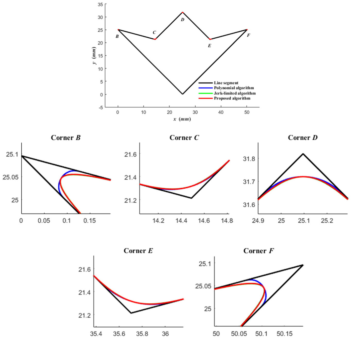
Trident-shaped trajectories and enlarged transition corner curves.

As shown in Figure 9(a), tangential velocities of the three algorithms are all smooth and below the specified federate F. In addition, as can be seen in Figure 9(b) and (c), the x-axis and y-axis velocities of the polynomial algorithm are not smooth at corners, while those of the jerk-limited algorithm are smooth. The axial acceleration and jerk profiles of these two comparison algorithms are also seen in Figure 9(d)–(g) to be significantly inferior as compared to the proposed algorithm. In Figure 9(d)–(g), the axial accelerations and jerks produced by the polynomial algorithm fluctuate frequently and exceed the specified limitations at corners due to the use of tangential kinematic constraints alone. And since the jerk-limited algorithm only guarantees the jerk-limited motion profiles under the axial kinematic limits, its axial accelerations are not smooth, and its axial jerks exhibits sudden changes at the corners. It can therefore be concluded that the synthesized motion profiles with the two comparison algorithms are more prone to causing vibration in the machine tool with the resulting surface quality issues. The proposed algorithm, on the other hand, has smooth axial velocity, acceleration and jerk profiles. The proposed algorithm should therefore achieve significantly better machining flexibility and machining quality.

Figure 9.

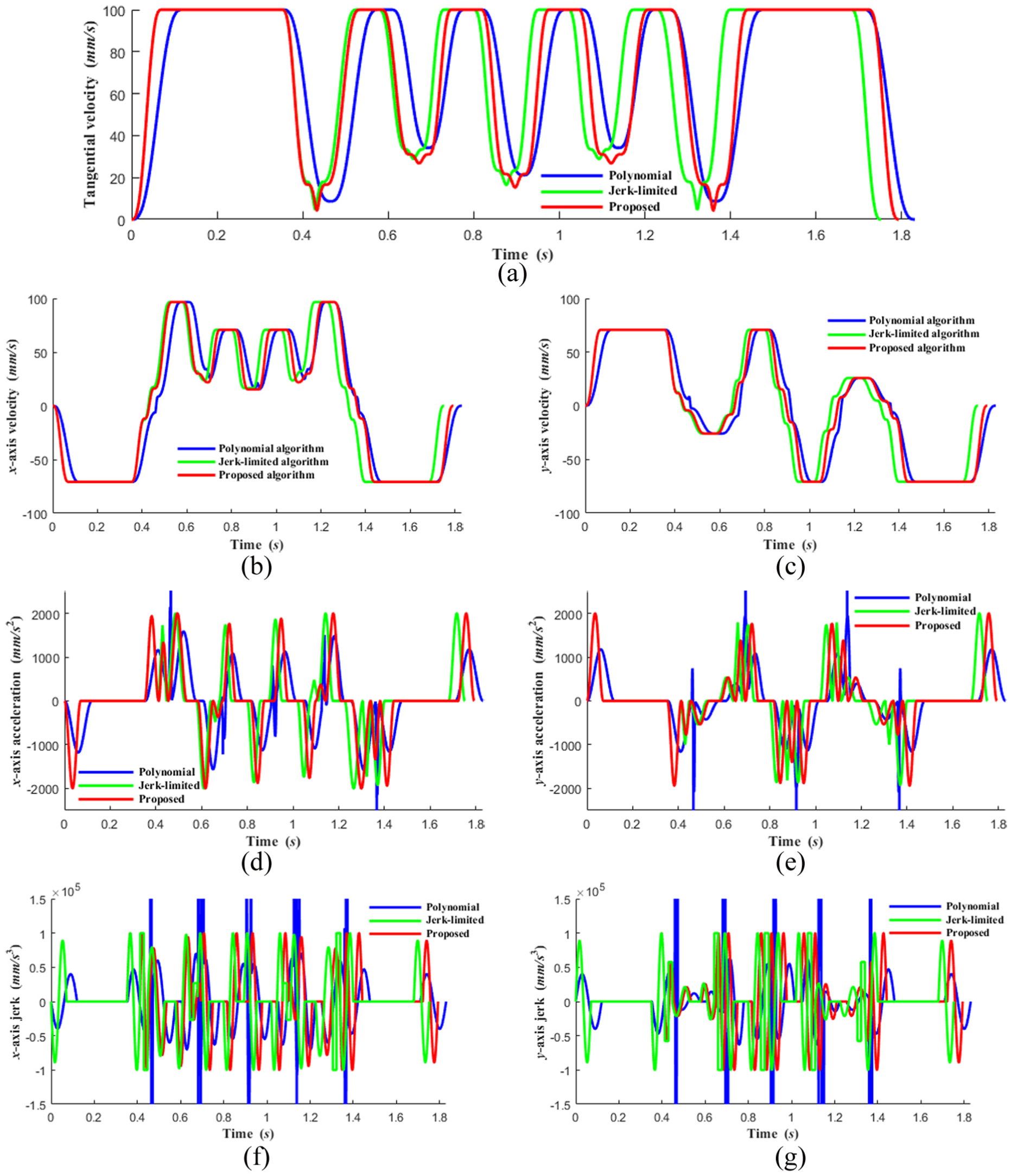
Comparison of the kinematic profiles for the Case 2: (a) tangential velocity profiles, (b) x-axis velocity profiles, (c) y-axis velocity profiles, (d) x-axis acceleration profiles, (e) y-axis acceleration profiles, (f) x-axis jerk profiles and (g) y-axis jerk profiles.

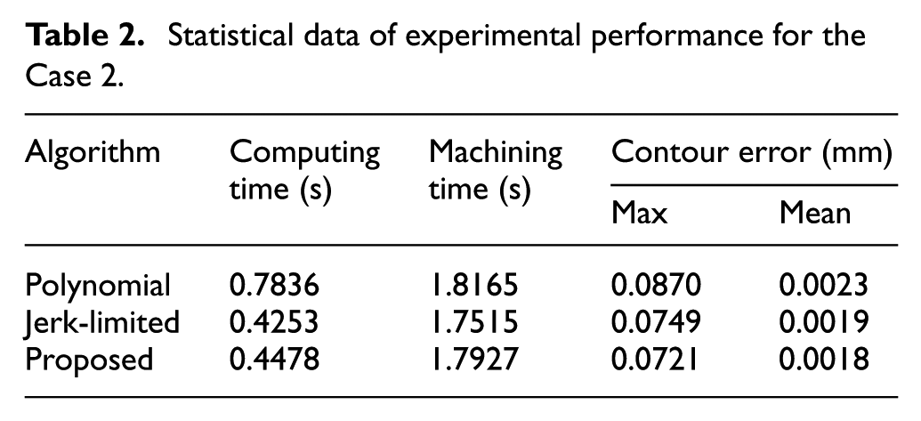
In Table 2, we can see that the machining time of the polynomial algorithm is the slowest at 1.8165 s, which is 1.3% and 3.7% slower than the proposed (1.7927 s) and jerk-limited (1.7515 s) algorithms, respectively. The computing time of the polynomial algorithm is 1.75 and 1.84 times longer than the proposed and jerk-limited algorithms, respectively. The reason for longer machining and computing time of the polynomial algorithm is due to separate tasks of constructing the transition curve and velocity planning, in which only the tangential kinematic limits are considered. Figure 10 shows the contour errors. As can be seen, large contour errors happen at the corners, but none of the three algorithms exceed the specified contour error ε.

Table 2.

Statistical data of experimental performance for the Case 2.

Algorithm	Computingtime (s)	Machiningtime (s)	Contour error (mm)
Algorithm	Computingtime (s)	Machiningtime (s)	Max	Mean
Polynomial	0.7836	1.8165	0.0870	0.0023
Jerk-limited	0.4253	1.7515	0.0749	0.0019
Proposed	0.4478	1.7927	0.0721	0.0018

Figure 10.

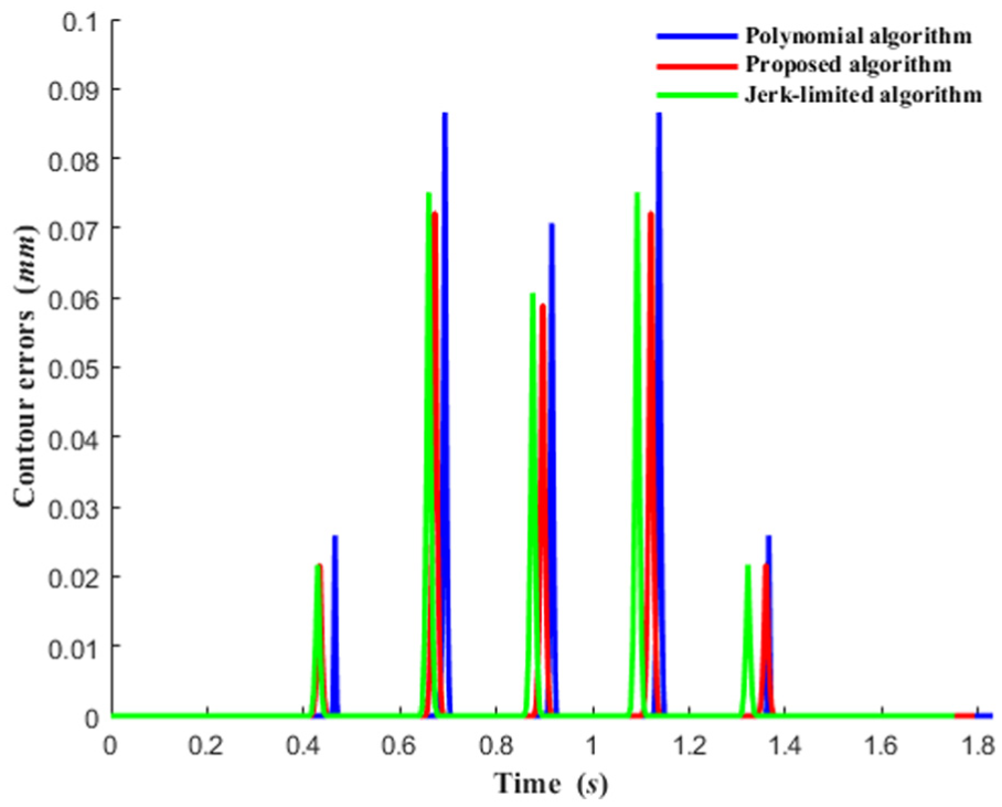
Contour errors for the Case 2.

As can be seen in Table 2, the maximum contour error of the proposed algorithm is 0.0721 mm, which is 17% and 3.7% less than the polynomial and jerk-limited algorithms, respectively. The mean contour errors of the proposed, polynomial and jerk-limited algorithms are 0.0018, 0.0023 and 0.0019 mm, respectively. So, the proposed real-time look-ahead interpolation algorithm with axial smooth transition scheme can also satisfy the requirement of machining accuracy and efficiency.

Case 3

In this case, a more complex pattern shown in Figure 11 is used for comparison of the performance of each of the above three algorithms. The pattern is closed and comprises 15 corners. The simulation conditions are the same as those of case 2. Similarly, the two-step quintic polynomial algorithm with the trigonometric velocity planning method¹⁹ and the axial jerk-limited transition algorithm³¹ are used for comparison and are referred to as the “polynomial algorithm” and “jerk-limited algorithm,” respectively.

Figure 11.

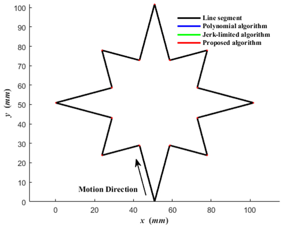
Star-shaped trajectories and synthesized transition curves.

The comparison of the simulation results is shown in Figures 12 and 13. From Figures 12(a) and 13, we can see that the tangential velocity curves of the three methods are smooth and below the programmed feedrate F, and that all the chord error curves are restricted to ε.

Figure 12.

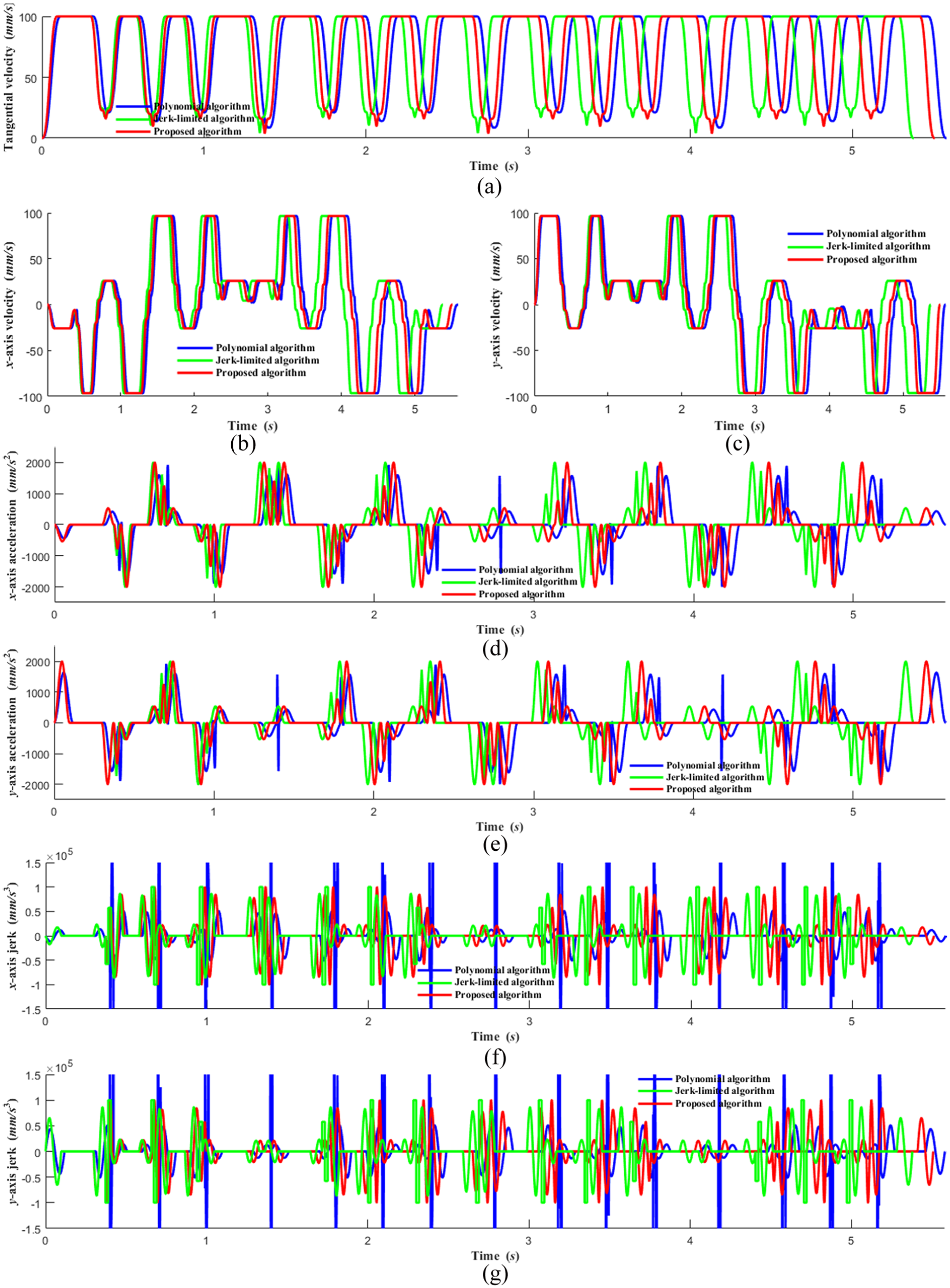
Comparison of the kinematic profiles for the Case 3: (a) tangential velocity profiles, (b) x-axis velocity profiles, (c) y-axis velocity profiles, (d) x-axis acceleration profiles, (e) y-axis acceleration profiles, (f) x-axis jerk profiles and (g) y-axis jerk profiles.

Figure 13.

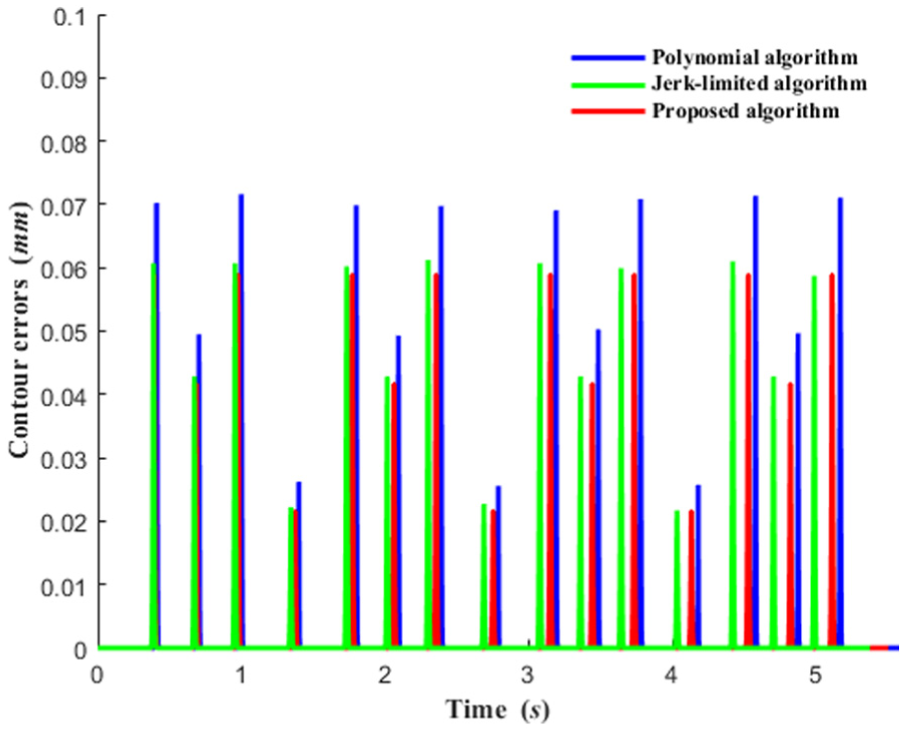
Contour errors for the Case 3.

However, in Figure 12(b) and (c), the axial velocity profiles of the polynomial algorithm are seen not to be smooth at the corners. In addition, Figure 12(d)–(g) shows that the polynomial algorithm axial accelerations and jerks fluctuate frequently and exceed the specified limitations at corners since the method only uses tangential velocity planning.

For the case of jerk-limited algorithm, its axial acceleration profiles are not smooth and its axial jerk curves change abruptly at the beginnings and ends of accelerating or decelerating periods at the corners.

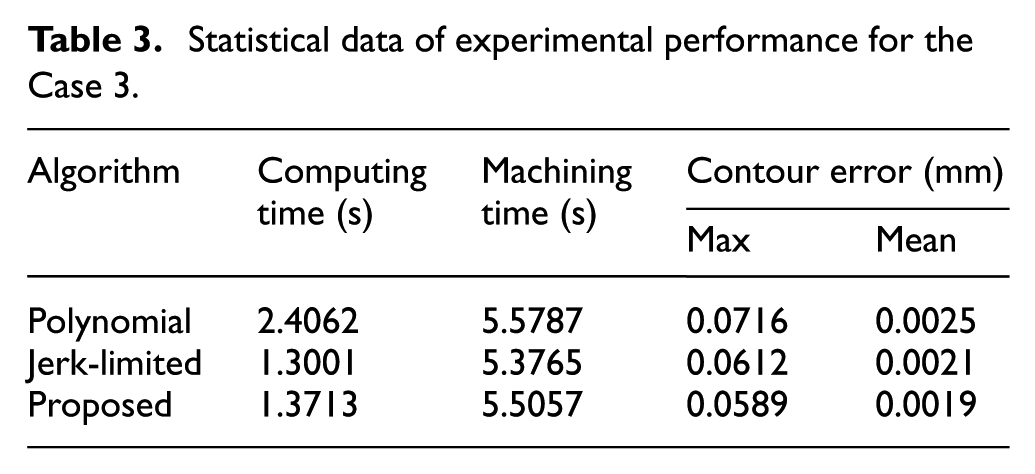
The proposed algorithm, however, is shown to provide smooth axial velocity, acceleration and jerk profiles during the entire motion, as can be seen in Figure 12. In Table 3, we can see that the polynomial algorithm requires close to twice the computing time of the proposed and jerk-limited algorithms. The machining time of the proposed algorithm is shown in Table 3 to be 5.5057 s, which is 2.4% slower than the jerk-limited algorithm (5.3765 s). However, it has a significantly reduced corner errors and should reduce machine tool vibration. It is therefore concluded that the proposed real-time look-ahead interpolation algorithm with axial smooth transition scheme can satisfy the requirements of machining efficiency and achieve a significantly better machining flexibility and machining quality.

Table 3.

Statistical data of experimental performance for the Case 3.

Algorithm	Computingtime (s)	Machiningtime (s)	Contour error (mm)
Algorithm	Computingtime (s)	Machiningtime (s)	Max	Mean
Polynomial	2.4062	5.5787	0.0716	0.0025
Jerk-limited	1.3001	5.3765	0.0612	0.0021
Proposed	1.3713	5.5057	0.0589	0.0019

Conclusion and discussions

In this article, a real-time and look-ahead interpolation algorithm with axial jerk-smooth transition scheme for CNC machining of micro-line segments is proposed. Transition curves and axial motion profiles are constructed in time domain simultaneously using the TVPM and look-ahead functions.

Compared to previous published work, the proposed algorithm has the following advantages. (1) The one-step process to obtain the transition curve and motion profiles improves the efficiency of the trajectory smoothing. The intersection of adjacent transition curves can also be avoided. (2) TVPM makes the calculation of kinematic functions easier and realizes the smooth axial velocity, acceleration and jerk control under chord error and drive axes constraints, noting that for high-speed machining, smooth axial motion profiles are more important than the tangential ones. (3) The look-ahead function guarantees the global feedrate profile and attainment of two corner velocities on every segment. In addition, due to the use of terminal condition, the look-ahead process can be terminated without scanning all the buffer units, which improves the efficiency of the look-ahead process.

The simulations are conducted to validate the feasibility and effectiveness of the proposed algorithm. The results show that the developed real-time and look-ahead interpolation algorithm with axial jerk-smooth transition scheme can achieve smooth trajectories and axial motion profiles and improve the smoothing process efficiency and achieve machining accuracy.

Future work will focus on two aspects. First, we are in the process of implementing the proposed algorithm on an open-source CNC 3-axis system and plan to publish the results shortly after. Second, more servo dynamics, such as jounce, is to be considered in the proposed algorithm.

Footnotes

Declaration of conflicting interests

The author(s) declared no potential conflicts of interest with respect to the research, authorship and/or publication of this article.

Funding

The author(s) disclosed receipt of the following financial support for the research, authorship, and/or publication of this article: This work was supported by the National Science and Technology Major Project of China (Grant No. 2017ZX04001001) and the China Scholarship Council (Grant No. 201704910554).

ORCID iD

Hao Li

References

Huang

Zhu

LM.

Feedrate scheduling for interpolation of parametric tool path using the sine series representation of jerk profile. Proc IMechE, Part B: J Engineering Manufacture 2017; 231(13): 2359–2371.

FANUC Corporation. FANUC series 30i/31i/32i/35i—Model B, https://www.fanuc.co.jp/en/product/catalog/pdf/cnc/FS30i-B(E)-09.pdf (2016, accessed 2 February 2018).

Siemens. Milling with SINUMERIK: mold making with 3 to 5-axis simultaneous milling, http://support.industry.siemens.com/cs/attachments/109740349/SIN_WF5_EN.pdf (2016, accessed 2 February 2018).

Zhang

Hong

et al . Research on smooth compression interpolation algorithm in CNC machining. J Mech Eng 2011; 47(5): 156–162.

Zhang

Guo

Gao

XS.

Cubic spline trajectory generation with axis jerk and tracking error constraints. Int J Precis Eng Manuf 2013; 14(7): 1141–1146.

Zhang

Song

TT.

Correcting and compressing interpolation algorithm for free-form surface machining. Int J Adv Manuf Techn 2012; 62(9–12): 1179–1189.

Bica

AM.

Optimizing at the end-points the Akima’s interpolation method of smooth curve fitting. Comput Aided Geom Des 2014; 31(5): 245–257.

Wang

Yang

Liu

YZ.

A real-time look-ahead interpolation algorithm based on Akima curve fitting. Int J Mach Tool Manuf 2014; 85(5): 122–130.

Zhang

et al . Fast parametric curve interpolation with minimal feedrate fluctuation by cubic B-spline. Proc IMechE, Part B: J Engineering Manufacture 2016; 232(9): 1624–1652.

10.

Wang

Liu

et al . Research of the real-time interpolation based on piecewise power basis functions. Proc IMechE, Part B: J Engineering Manufacture 2019; 233(3): 889–899.

11.

Liu

Jia

et al . Interpolation using non-uniform rational B-spline for the smooth milling of ruled-surface impeller blades. Proc IMechE, Part B: J Engineering Manufacture 2015; 229(7): 1118–1130.

12.

Yang

Shen

Yuan

et al . Curve fitting and optimal interpolation for CNC machining under confined error using quadratic B-splines. Comput Aided Des 2015; 66(C): 62–72.

13.

Zhao

Zhu

et al . Look-ahead interpolation of short line segments using B-spline curve fitting of dominant points. Proc IMechE, Part B: J Engineering Manufacture 2014; 229(7): 1131–1143.

14.

Zhao

Wang

et al . A data compression algorithm based on G2 continuous Bézier curves for tool paths. J Shanghai Jiaotong Univ 2014; 48(5): 629–635.

15.

Wang

Yau

HT.

Real-time NURBS interpolator: application to short linear segments. Int J Adv Manuf Techn 2009; 41(11–12): 1169–1185.

16.

Lee

Hascoet

JY.

Smooth circular arc interpolation for planar free curves with tolerance control. Proc IMechE, Part B: J Engineering Manufacture 1999; 213(6): 629–634.

17.

Zhang

Zhou

LS.

Adaptive algorithm for feedrate smoothing of high speed machining. Acta Aeronaut Astronaut Sin 2006; 27(1): 125–130.

18.

Zhang

Yang

et al . Study on the method of increasing turning velocity during CNC continuous machining. Manuf Technol Mach Tool 2008; 7: 79–83.

19.

Zhang

Yang

et al . Corner curve transition interpolation algorithm for high speed machining of micro-line segment. J Mech Eng 2010; 46(19): 183–191.

20.

Ernesto

Farouki

RT.

High-speed cornering by CNC machines under prescribed bounds on axis accelerations and toolpath contour error. Int J Adv Manuf Techn 2012; 58(1–4): 327–338.

21.

Sencer

Ishizaki

Shamoto

A curvature optimal sharp corner smoothing algorithm for high-speed feed motion generation of NC systems along linear tool paths. Int J Adv Manuf Techn 2015; 76(9–12): 1977–1992.

22.

Huang

Zhu

LM.

A locally optimal transition method with analytical calculation of transition length for computer numerical control machining of short line segments. Proc IMechE, Part B: J Engineering Manufacture 2017; 232: 2409–2419.

23.

Yutkowitz

Chester

Apparatus and method for smooth cornering in a motion control system. Patent 6922606, USA, 2005

24.

Zhao

Zhu

Ding

A real-time look-ahead interpolation methodology with curvature-continuous B-spline transition scheme for CNC machining of short line segments. Int J Mach Tool Manuf 2013; 65(2): 88–98.

25.

Fan

Lee

Chen

JH.

A realtime curvature-smooth interpolation scheme and motion planning for CNC machining of short line segments. Int J Mach Tool Manuf 2015; 96: 27–46.

26.

Sencer

Ishizaki

Shamoto

High speed cornering strategy with confined contour error and vibration suppression for CNC machine tools. CIRP Ann Manuf Tech 2015; 64(1): 369–372.

27.

Biagiotti

Melchiorri

FIR filters for online trajectory planning with time- and frequency-domain specifications. Control Eng Pract 2012; 20(12): 1385–1399.

28.

Zhang

Sun

Gao

et al . High speed interpolation for micro-line trajectory and adaptive real-time look-ahead scheme in CNC machining. Sci China Technol Sci 2011; 54(6): 1481–1495.

29.

Tsai

Huang

YC.

A novel integrated dynamic acceleration/deceleration interpolation algorithm for a CNC controller. Int J Adv Manuf Techn 2016; 87(1–4): 279–292.

30.

Duan

Okwudire

Minimum-time cornering for CNC machines using an optimal control method with NURBS parameterization. Int J Adv Manuf Techn 2016; 85(5–8): 1405–1418.

31.

Tajima

Sencer

Kinematic corner smoothing for high speed machine tools. Int J Mach Tool Manuf 2016; 108: 27–43.

A real-time and look-ahead interpolation algorithm with axial jerk-smooth transition scheme for computer numerical control machining of micro-line segments

Abstract

Keywords

Introduction

Transition scheme

Trigonometric velocity planning method

Transition construction scheme with prescribed chord error and axial jerk-smooth motion profiles

Real-time interpolation with look-ahead function

Look-ahead initialization

Backward scanning

Simulation validations

Case 1

Case 2

Case 3

Conclusion and discussions

Footnotes

Declaration of conflicting interests

Funding

ORCID iD

References