
Abstract
Single-point incremental forming is a novel and flexible method for producing three-dimensional parts from metal sheets. Although single-point incremental forming is a suitable method for rapid prototyping of sheet metal components, there are limitations and challenges facing the commercialization of this process. Dimensional accuracy, surface quality, and production time are of vital importance in any manufacturing process. The present study is aimed at selecting proper forming parameters to produce sheet metal parts which possess dimensional accuracy and good surface quality at the shortest time. Four parameters (i.e. tool diameter, tool step depth, sheet thickness, and feed rate) are chosen as design variables. These parameters are used for the modeling of the process using Group Method of Data Handing(GMDH) artificial neural networks. The data necessary for establishing empirical models are obtained from single-point incremental forming experiments carried out on a computer numerical control milling machine using central composite design. After the evaluation of the model accuracy, single- and multi-objective optimization are performed via genetic algorithm. The performance of the design variables of a tradeoff point corresponding to one of the experiments shows the efficiency and accuracy of the models and the optimization process. Considering the priorities of objective functions, a designer will be able to set proper process parameters.
Keywords
Introduction
Single-point incremental forming (SPIF) is an innovative and flexible method for making symmetrical and asymmetrical parts from metal sheets at the shortest time and lowest cost. This method is completely different from conventional methods, and the equipment it requires includes a smooth semi-spherical headed tool and a frame for sheet clamping. The final geometry of the part is gradually obtained from the interface between the semi-spherical headed tool and the sheet along a spiral path consisting of different sections of the part. A computer numerical control (CNC) milling machine creates the movement of the tool and its path. SPIF is a flexible process, and its formability is higher than that of conventional methods. 1 Although this method has many advantages, its application in the industry faces with limitations and challenges. Not only is it time-consuming, but the dimensional and geometrical accuracy of produced parts is insufficient. In fact, the simplicity of the equipment and the mechanics of the process decrease dimensional accuracy. 2 Figure 1 shows three types of geometrical errors in a final part, including unwanted plastic deformation, spring-back, and pillow effect. Since the largest section of the sheet is not clamped during forming, the final geometry may be different from the Computer Aided Design (CAD) model in many ways. 3 This is as a result of the elastic spring-back and unwanted rigid movement of the sections of the sheet due to the nature of this process which has no die and can create problems in cases where a high level of accuracy is required. 4 The following methods have been used to reduce geometrical error in SPIF:
Setting proper values or optimization of the pertinent parameters (e.g. tool diameter, step depth, and feed rate);2,5,6
Adopting multistage rather than single-stage forming strategies;4,7–9
Choosing different strategies of tool paths such as reforming from the reverse side of the part or forming in the tool’s clockwise path first and the tool’s counter-clockwise path next;8,9
Locally heating the forming zone; 13
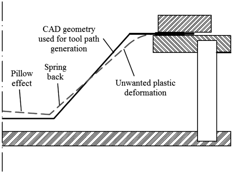
Types of geometrical errors during single-point incremental forming.
Each of the methods mentioned above has been effective in reducing error, but further research is required to achieve acceptable dimensional accuracy for the parts manufactured via traditional methods of sheet forming.
In order to keep the main feature of tooling simplicity, the best way to reduce the geometrical error and thus increase the part accuracy is to modify the tool paths different from the one produced by the CAD model able to take into account both spring-back effects and stiffness reduction due to specific clamping equipment. 17 This is not readily possible because material behavior is not linear and depends on different parameters. 2 Furthermore, despite the fact that the deformation caused by the SPIF tool is local, its after-facts are not localized. 18 No matter the method used for increasing dimensional accuracy, efficiency is enhanced if proper forming parameters are set.
Studies have shown that selection of design variables for improving geometrical accuracy increases processing time and reduces surface quality. The surface roughness of the part is one of the most important quality indices in manufacturing. This parameter is very significant in incremental forming, particularly in medical applications, automobile industry and in cases where the appearance of components is an issue. Despite the importance of the surface quality of the parts manufactured in SPIF, little research has been conducted on the effect of process parameters on surface quality. Hagan and Jeswiet 19 studied the impact of step depth and spindle speed on mean surface roughness and mean peak-to-valley height and concluded that spindle speed has little effect on surface roughness. Moreover, they presented an analytical model for estimating the mean peak-to-valley height of incrementally formed parts. Bhattacharya et al. 20 investigated the effect of process parameters on obtaining the maximum formable wall angle and the best surface quality. They developed an empirical model for estimating mean surface roughness and maximum formable wall angle as functions of process parameters. Mugendiran et al. 21 studied the influence of the three parameters: spindle speed, feed rate, and step depth on the surface roughness and wall thickness of the components made from aluminum 5052. They optimized parameters via response surface methodology (RSM) such that the manufactured parts had maximum wall thickness and minimum roughness. Shanmuganatan and Senthil Kumar 22 studied the impact of tool diameter, step depth, feed rate, and spindle speed on three output parameters: maximum formable wall angle, mean wall thickness, and surface roughness. They defined output parameters as a function of input parameters by developing a mathematical model. Durante et al. 23 presented an analytical equation for the three roughness parameters: RSM, Ra, and Rz as functions of step depth, wall angle, and tool diameter, respectively. Kurra et al. 24 modeled surface roughness using artificial neural network (ANN), support vector regression (SVR), and genetic programming (GP). These approaches considered tool diameter, step depth, wall angle, feed rate, and lubricant type as input variables. Moreover, mean surface roughness (Ra) and mean maximum peak-to-valley height (Rz) were considered as response variables. They found that the SVR model yields better results as compared to the other models in predicting Ra and Rz. Furthermore, the model developed through GP was employed with the aim of minimizing surface roughness.
Another limitation of this process is that incremental forming is time-consuming.17,25 Given the simple mechanism required by incremental forming, the only factor that contributes to manufacturing cost is the time required for forming. Forming time (FT) is very important, especially when the dimensions of the part are considered. However, FT has not been studied in the literature as a key manufacturing criterion, and this triggered the present study. Preliminary experiments revealed that reducing the values of some process parameters such as step depth and feed rate reduces surface roughness but significantly increases FT. In addition, increasing tool diameter improves surface quality but reduces dimensional accuracy. This confuses the designer when selecting the parameters.
Considering the contradictory effects of some input parameters on dimensional accuracy, surface roughness, and FT, the present study first proposes a mathematical model for estimating geometrical error, surface roughness, and the time required for forming as functions of process parameters using the Group Method of Data Handing (GMDH) method. The input parameters are step depth, feed rate, tool diameter, and sheet thickness. The motivation behind the inclusion of sheet thickness as a parameter is that its effect on surface roughness has not been studied before. Then, genetic algorithm (GA) is used for both single and multi-objective optimization of the objective functions. A tradeoff point is then selected from the Pareto front such that maximum dimensional accuracy and surface quality are obtained at the shortest time. The data required for empirical models are prepared in a series of experiments via central composite design (CCD).
Methodology
Materials and forming equipment
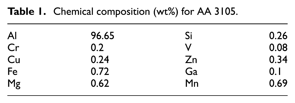
AA3105 aluminum alloy blanks with a size of 180 × 180 mm and a thickness of 0.5, 1, and 1.5 mm were prepared and then annealed to ensure uniformity of mechanical structure. The chemical structure of this alloy is shown in Table 1. The initial arithmetic mean surface roughness value (Ra) of each blank is 0.31 µm.
Chemical composition (wt%) for AA 3105.
To carry out the experiments, a CNC milling machine (model VMC850 with a Siemens controller) was used. The maximum spindle speed of the machine is 8000 r/min, and its electromotor power is 12 kW. This machine has a maximum table travel of 800 × 500 × 600 mm in X, Y, and Z directions, respectively. Each blank was formed in a single stage with the movement of the tool center along a spiral path generated by a CAD/CAM software program. Vertical step depth was between 0.2 and 1 mm, and feed rate was between 600 and 1400 mm/min. Hydraulic oil was used as a lubricant during forming. To make sure the forming conditions are constant, the rolling direction of the sheet was kept along the y-axis of the CNC machine. In addition, to ensure the parts are measured under identical conditions, the rolling direction of the sheet was kept along the y-axis of the coordinate measuring machine (CMM). As shown in Figure 2, the geometry under study is a frustum with a square base of 140 × 140 mm and a height of 50 mm. A main source of error is unwanted plastic deformation due to high stress levels in areas adjacent to the contact region of the tool. This deformation is seen particularly in the vicinity of steep slopes. 26 To study unwanted plastic deformation, a size of 160 × 160 mm is considered for the internal space of the backing plate. This means that a strip with a width of 10 mm is without support. The use of tools with larger diameters reduces formability. 27 In addition, tools with smaller diameters increase dimensional accuracy at wider wall angles. 5
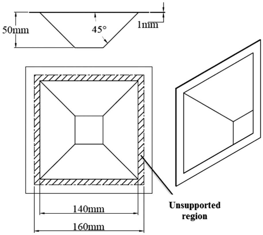
The tested pyramid dimensions and unsupported region.
Most studies usually adopt a tool diameter of between 4 and 12 mm. For the purpose of the present study, semi-spherical headed tools with diameters of 5, 9, and 13 mm were made from SPK steel following the 1.2080 standard. A clamping mechanism with a workspace of 250 × 250 mm was designed. To keep the total temperature of the part constant, a cooling liquid spray was directed at the back of the blank during the forming process. This was performed because in the absence of cooling, the total temperature of the part would increase and upon completion of the process, the part would contract because its temperature is equal to the ambient temperature, thereby severely reducing dimensional accuracy. Figure 3 shows the equipment used in the experiments.
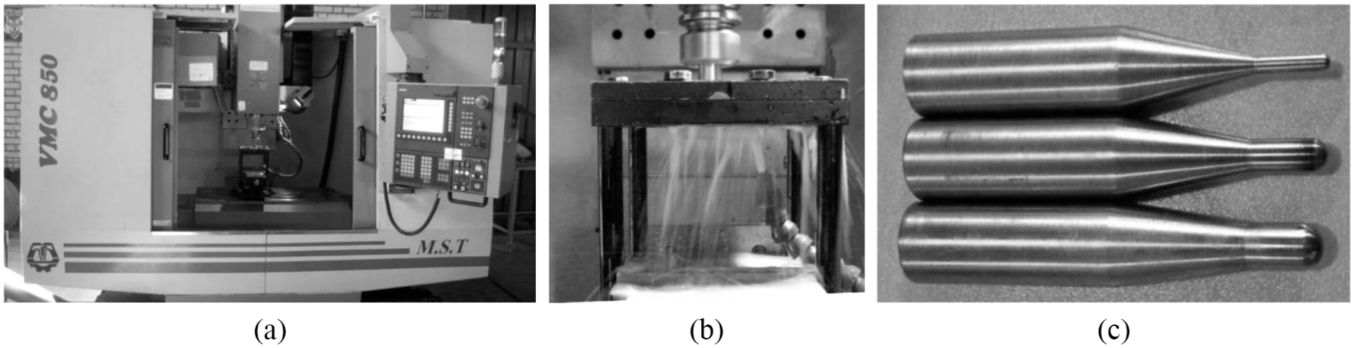
(a) Three-axis CNC milling for incremental forming, (b) spraying a cooling liquid on the back of the plate to keep the overall temperature of the part constant, and (c) semi-spherical headed tools with diameters of 5, 9, and 13 mm.
Measurement of dimensional error, surface roughness, and FT
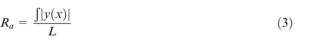
After forming, the height of the manufactured parts was measured using a CMM along a vertical plane that is perpendicular to the direction of sheet rolling and crossed the center of the part. The measurement was performed at 26 equally spaced points over the entire profile, except the bottom. The clamping mechanism was retained at the time of measuring the part on the CMM (Figure 4). At each point, the height of the manufactured part was compared with the corresponding point of the designed profile, and the discrepancy between the two was expressed as mean error using equation (1)
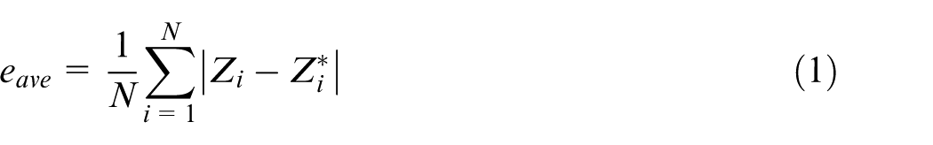
where
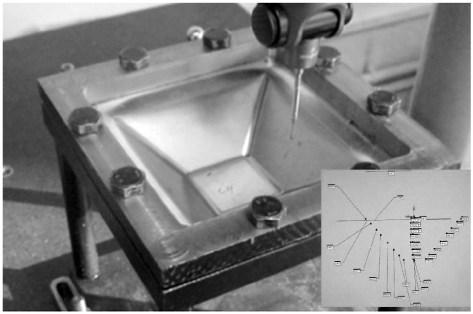
Measuring the formed part using coordinate measuring machine.
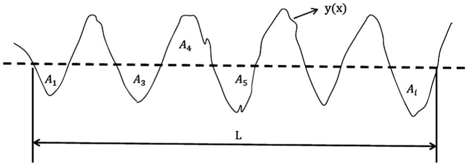
The schematic representation of roughness profile.
Considering Figure 5,
The surface roughness of the formed parts was measured using a roughness tester (Mitutoyo model SJ301) (Figure 6). To increase accuracy, each part was measured three times, and the average value was adopted as the surface roughness of the manufactured part. FT was calculated using the CAD/CAM software.
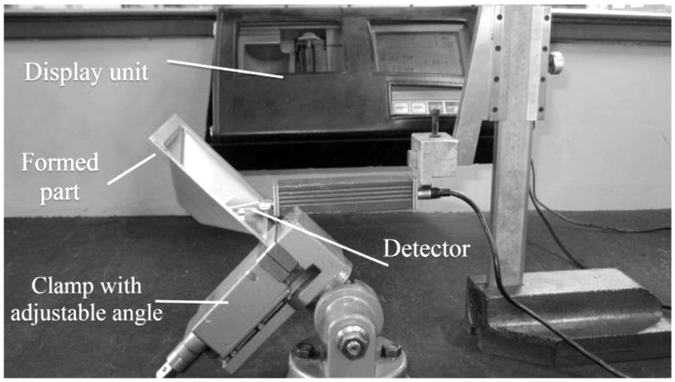
Experimental setup for surface roughness measurement.
Design of experiments
Design of experiment (DOE) methods are employed in order to select the optimum number of experiments used to study the effect of process parameters on the output. DOE techniques significantly affect the accuracy and cost of experiments. These techniques make it possible to study the individual effects of each variable and also their collective effects. 28
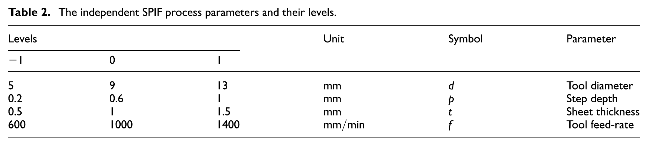
Tool diameter, step depth, wall angle, spindle speed, feed rate, and lubricant type have effect on surface roughness.21,23,24 Dimensional accuracy is affected by sheet thickness, tool diameter, wall angle, final part depth, and step depth.2,5 Tool diameter (d), step depth (p), sheet thickness (t), and feed rate
The independent SPIF process parameters and their levels.
Design of 30 experiments according to the CCD method and the corresponding results.
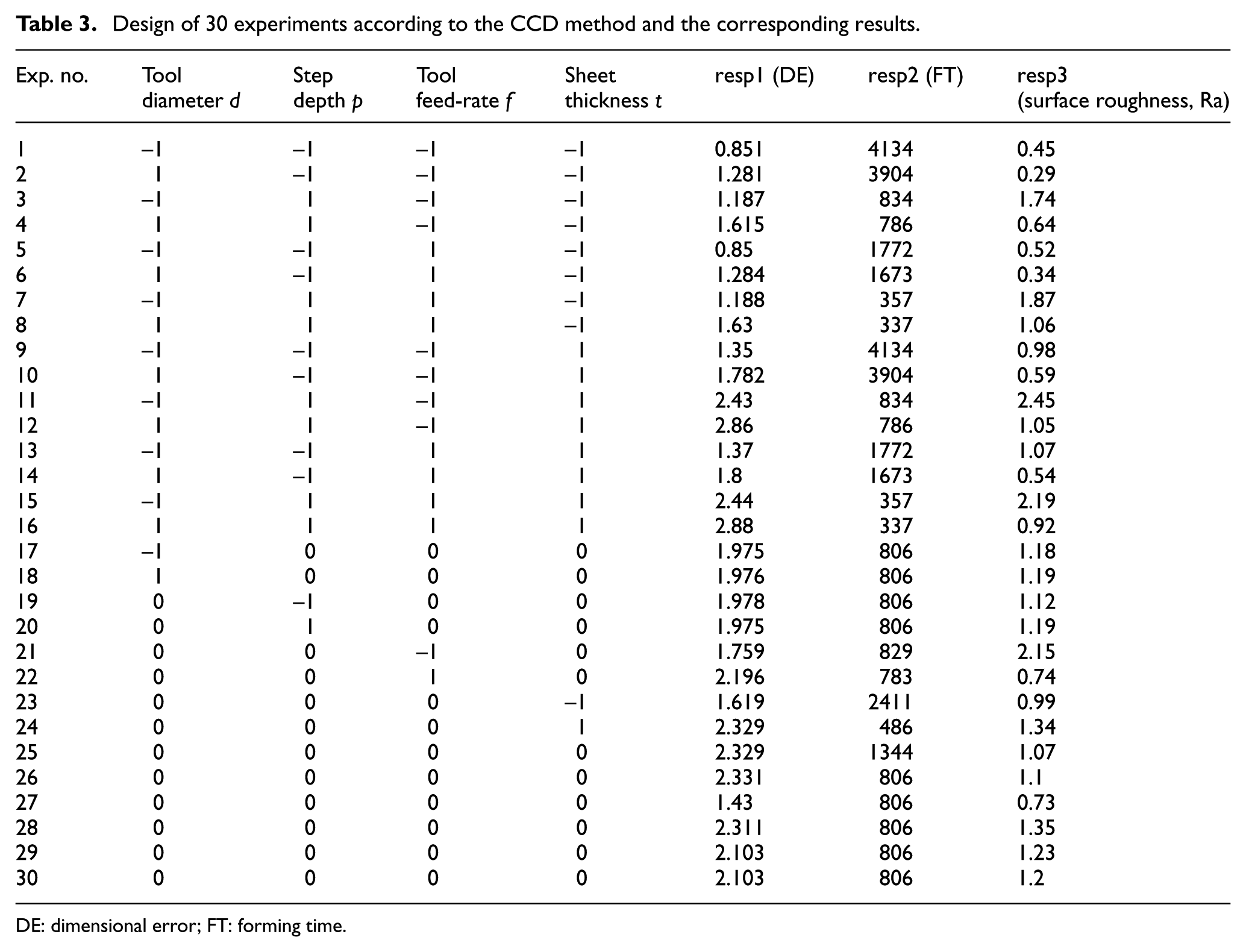
DE: dimensional error; FT: forming time.
The effect of forming parameters on SPIF
Effect of the four parameters: tool diameter, sheet thickness, tool feed-rate, and step depth, on dimensional accuracy, surface roughness and FT without considering the middle levels, are shown in Figure 7. Figure 7(a) reveals that sheet thickness, whose effect on surface roughness has not been examined in any research, is a key parameter such that when it increases, the surface roughness also increases. This effect is more intense with a smaller tool diameter. The increase in tool diameter causes greater overlap between the successive contours which lead to better surface finish. 29 Figure 7(b) shows that increasing step depth and tool feed-rate leads to an increase in surface roughness. The effect of tool feed-rate is not significant, but that of step depth is significant. Geometrically, tool feed-rate has no effect on surface roughness. Experiments show that increased surface roughness caused by increased tool feed-rate is associated with tool run-out. Figure 7(c) demonstrates that tool feed-rate does not affect the DE. However, when sheet thickness is increased, DE also increases. Figure 7(d) illustrates that reducing both tool diameter and step depth improve profile accuracy. As expected, FT is not affected by sheet thickness. Tool diameter has little effect on FT, and FT is strongly influenced by step depth and tool feed-rate (Figure 7(e) and (f)). Step depth has the greatest impact on FT, which is due to great reduction in the number of contours as a result of increase in step depth and a corresponding decrease in the total length of the tool path. 29
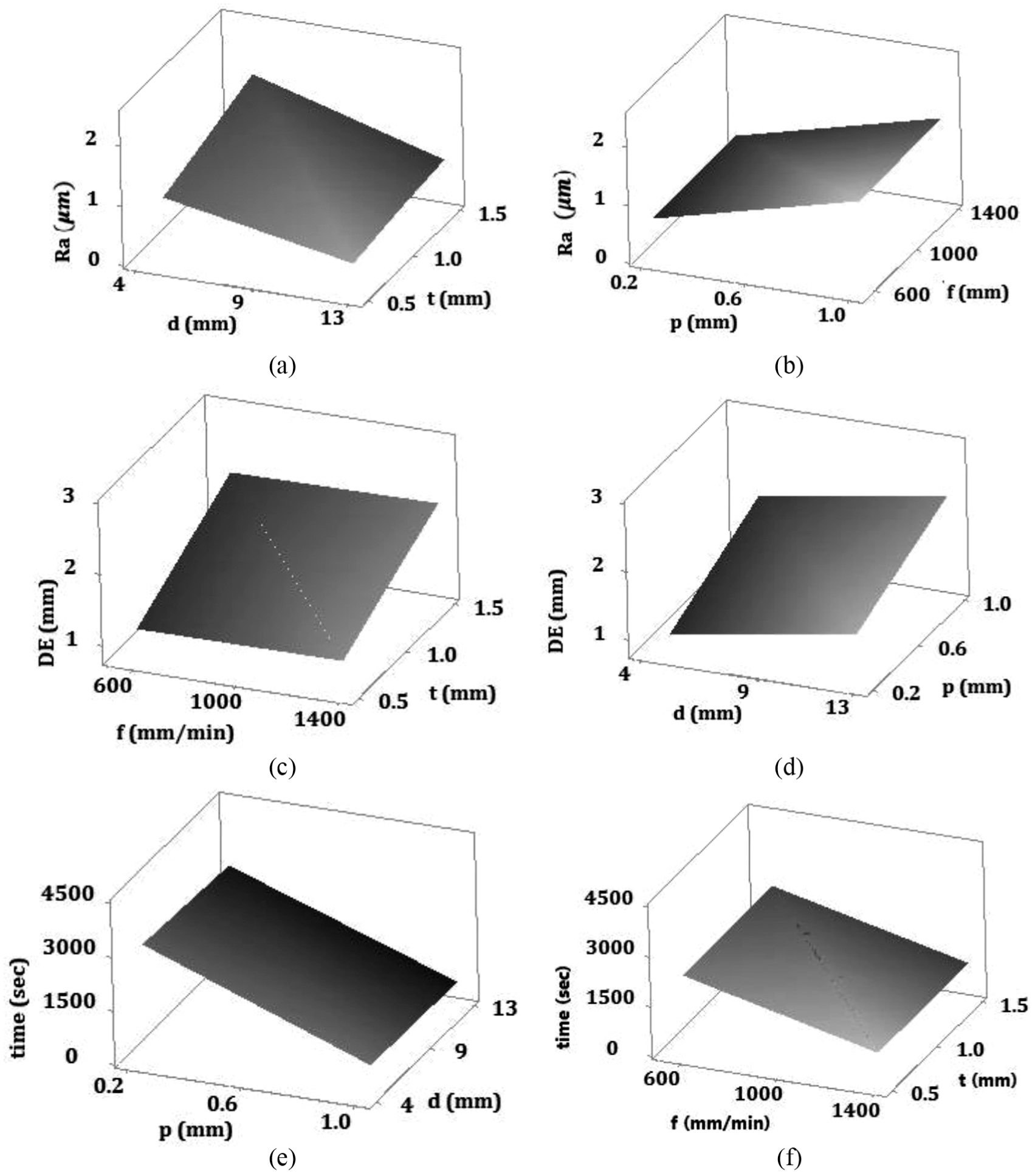
The plots of the effect of the study parameters on SPIF (a) The effect of the sheet thickness and tool diameter on surface roughness. (b) The effect of step depth and tool feed-rate on surface roughness. (c) The effect of sheet thickness and tool feed-rate on dimensional error. (d) The effect of step depth and tool diameter on dimensional error. (e) The effect of tool diameter and step depth on forming time. (f) The effect of sheet thickness and tool feed-rate on forming time.
Table 4 shows the generally contradictory behavior of output parameters in reaction to an increase in the values of input parameters.
The behavior exhibited by output parameters in reaction to the increase in the values of input parameters.
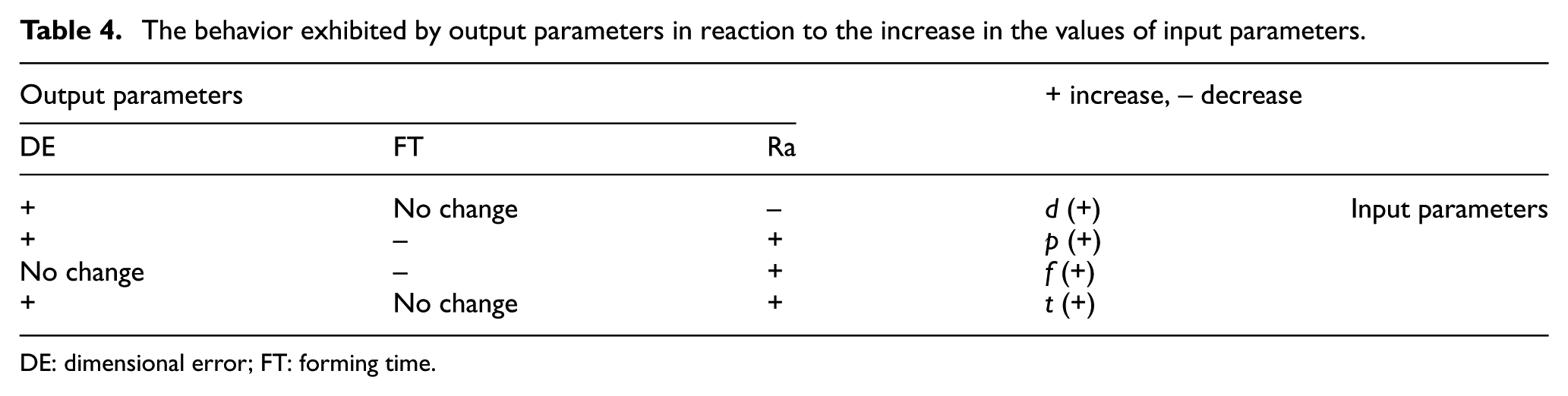
DE: dimensional error; FT: forming time.
Modeling using GMDH-type neural networks
Using the GMDH algorithm, a model can be developed as a set of neurons where different pairs are connected in each layer through a quadratic polynomial and therefore produce new neurons in the next layer. Such representation can be employed in modeling in an attempt to map inputs onto outputs. The formal definition of the identification problem is to find a function

we can now train a GMDH-type neural network to predict the output values

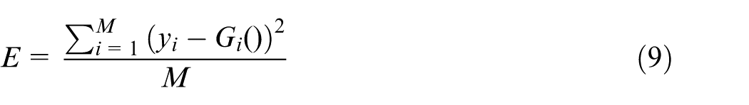
The problem now is to determine a GMDH-type neural network so that the square of the differences between the actual and predicted output can be brought to a minimum. That is to say
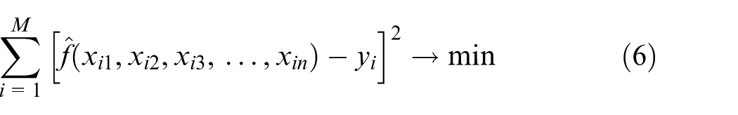
The general relationship between inputs and output variables can be indicated via a complicated discrete form of
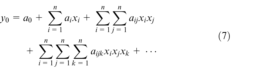
which is referred to as the Kolmogorov–Gabor polynomial. 29 This full form of mathematical expression can be presented through the use of a system of partial quadratic polynomials consisting of only two variables (neurons) in the form of
Thus, such partial quadratic description is recursively used in a network of connected neurons to establish the general mathematical relation between the input and output variables given in equation (7). The coefficients
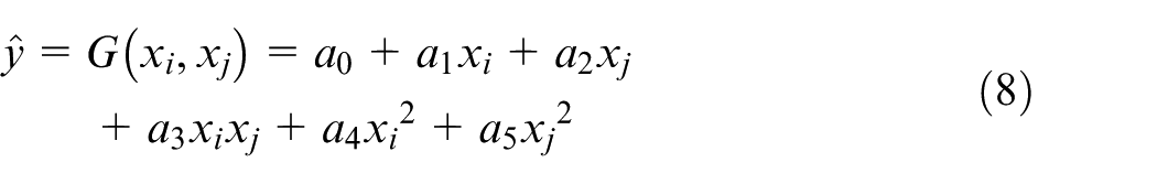
In the basic form of the GMDH algorithm, it is taken into account that all the possibilities of two independent variables out of the total n input variables in an effort to construct the regression polynomial in the form of equation (8) that best fits the dependent observations
GMDH-type meta-model for DE
Figure 8(a) depicts the structure of the evolved two-hidden layer GMDH-type neural network of DE. The corresponding recursive polynomial representation of the model for DE is given in equation (10)
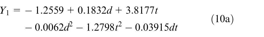
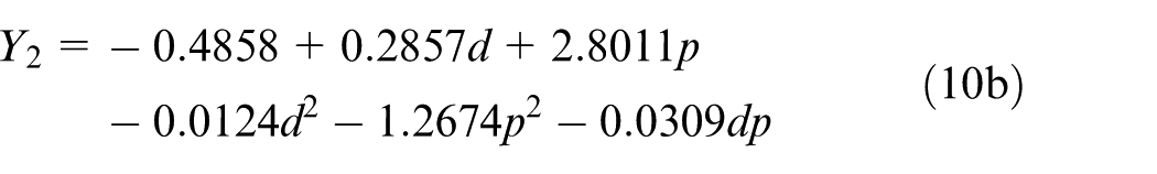
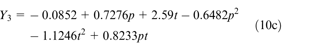
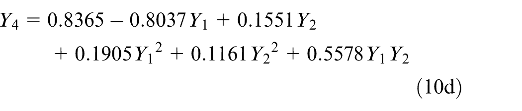
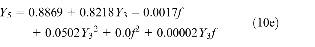
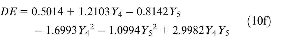
(a) The structure of the evolved two-hidden layer GMDH-type neural network of DE and (b) scatter diagram of the experimental values versus estimated values of DE.
In order to show the favorable precision of the constructed meta-model, the scatter diagram of experimental values versus estimated values is given in Figure 8(b). Also presented is a statistical measure based on R2 as the absolute fraction of variance. It is obvious from Figure 8(b) that the constructed GMDH-type neural network is well trained and also has good prediction ability.
GMDH-type meta-model for FT
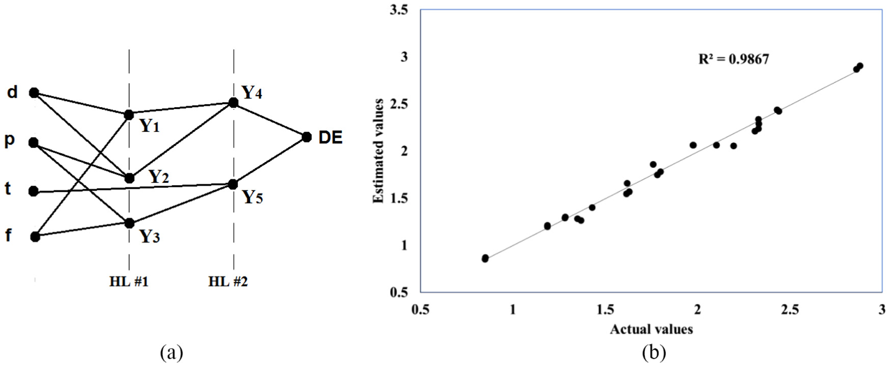
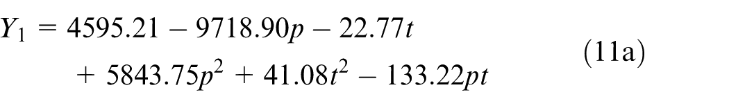
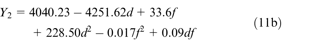
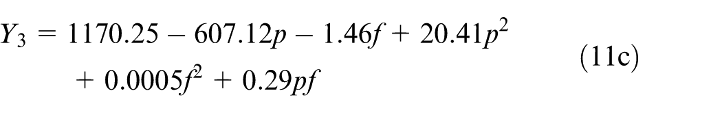
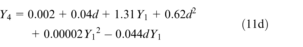
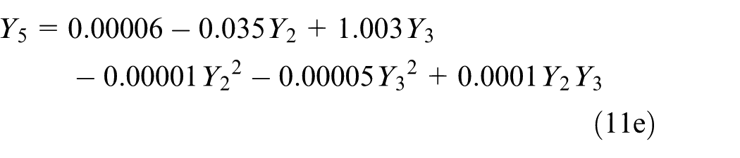
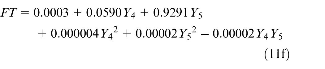
Figure 9(a) illustrates the structure of the two-hidden layer GMDH-type neural network of FT. The recursive polynomial representation of the model for FT is given in equation (11). Figure 9(b) is the scatter diagram of the experimental values versus estimated values of FT
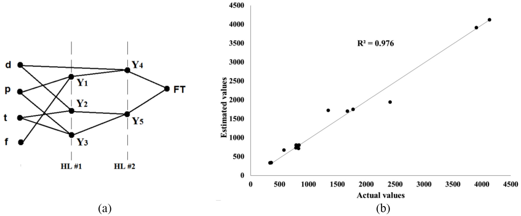
(a) The structure of the two-hidden layer GMDH-type neural network of FT and (b) scatter diagram of the experimental values versus estimated values of FT.
GMDH-type meta-model for Ra
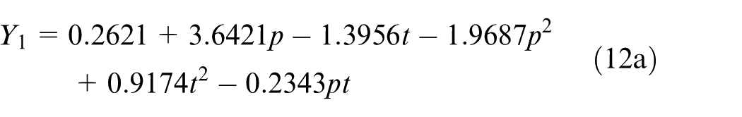
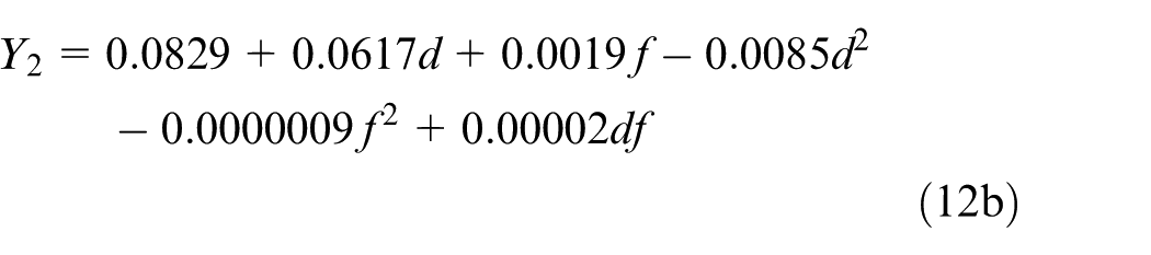
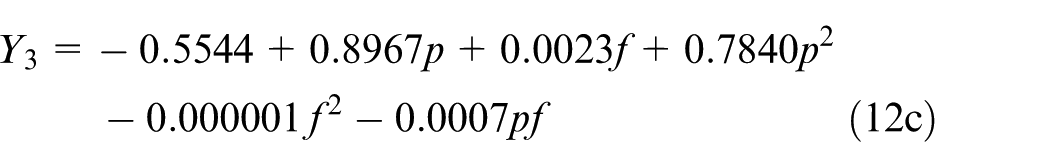
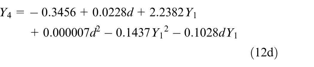
The structure of the two-hidden layer GMDH-type neural network of Ra is presented in Figure 10(a). The corresponding recursive polynomial representation of this model is given in equation (12). Moreover, the scatter diagram of the experimental values versus estimated values of Ra is given in Figure 10(b)
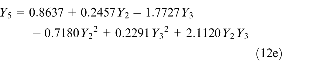
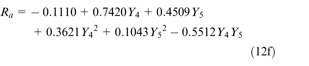
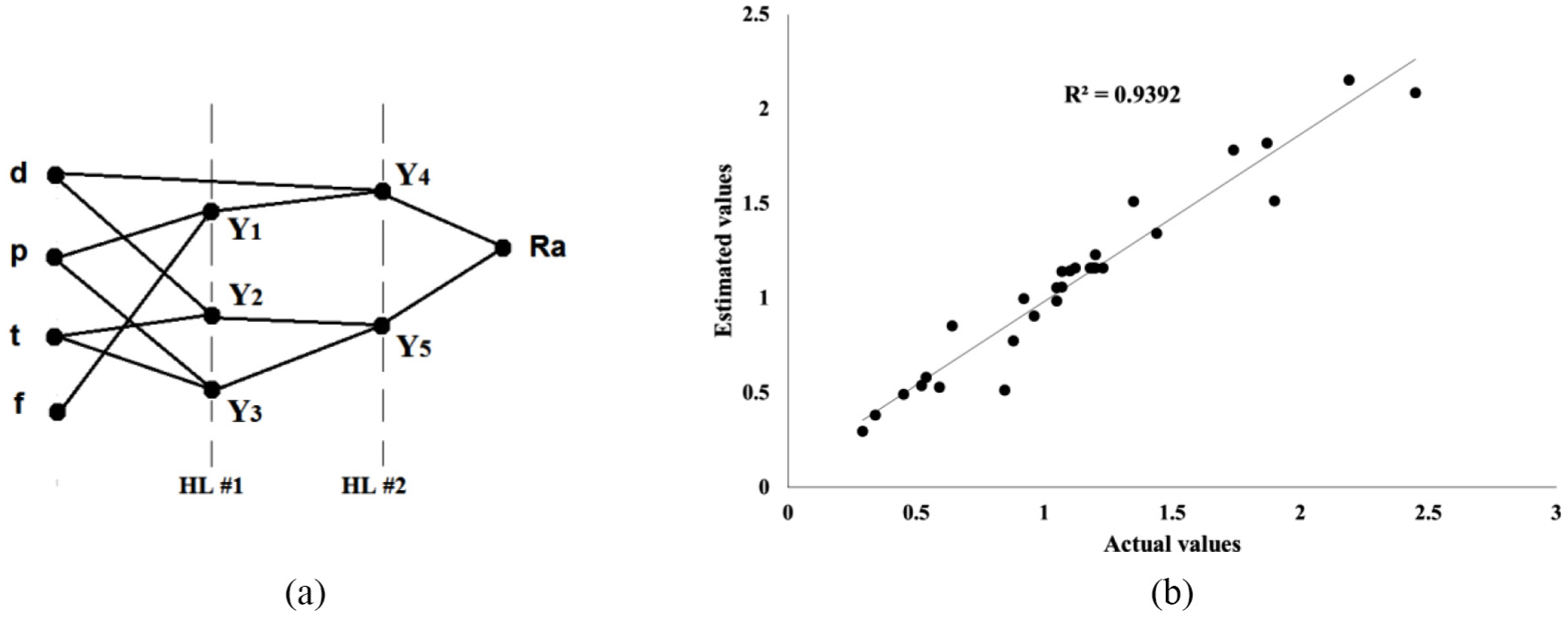
(a) The structure of the two-hidden layer GMDH-type neural network of Ra and (b) scatter diagram of the experimental values versus estimated values of Ra.
Single- and multi-objective optimization
Generally, a set of the design variables are determined in the optimization of SPIF processes such that objective functions have a favorable value of optimality. The objective functions are formable angle, wall thickness, surface roughness, and dimensional accuracy. In the present study, heuristic models were developed on the basis of the GMDH-type ANNs for the objective functions of FT, DE, and Ra using some experimental data. These models are used as objective functions in the process of single- and multi-objective optimization. In this way, the upper and lower bounds of the design variables are given below. For the purposes of GA, initial population, number of iterations, mutation probability, and linkage probability were assumed as 80, 250, 0.03, and 0.9, respectively


To show some contradictory effects of the design variables on objective functions, both two- and three-objective optimizations were performed in addition to single-objective optimization. The optimization process was programmed using GA on the MATLAB software.
Single-objective optimization
Single-objective optimization aims to minimize an objective function when FT, DE, and Ra are in separate optimization process. Table 5 shows the optimal values of the objective functions and their SPIF parameters. Evidently, single-objective minimization of each objective function results in non-favorable values for the other objective functions. For example, adjustment of the design variables for the purpose of minimizing the DE increases FT.
Optimization results of GA.
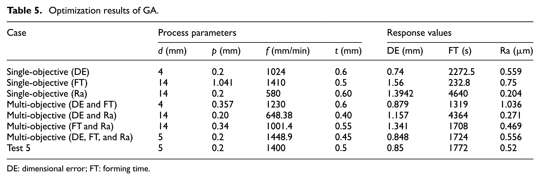
DE: dimensional error; FT: forming time.
Also, adjustment of the design variables with the aim of reducing FT significantly increases surface roughness and DE. In addition, a study on single-objective optimizations of surface roughness shows that the best surface quality can be obtained at the lowest sheet thickness.
Multi-objective optimization
In fact, single-objective optimization does not lead to the simultaneous optimization of DE, FT, and surface roughness, which can be attributed to the contradictory behavior of these objective functions. Some non-dominated solutions exist as optimal solutions which can be used to find some tradeoff points. 35 Such Pareto-based method was employed for multi-objective optimization of this process. In this way, these objective functions were optimized two at a time. Then, the three objective functions were optimized simultaneously.
Two-objective optimization
Table 5 shows the results obtained from Pareto-based two-objective optimization. Among the Pareto points, one was selected as the tradeoff point (Figures 11–13). As shown in Table 5, the optimal values of DE and FT are 0.88 mm and 1319 s, respectively. By substituting optimal design variables in equation (6), a predicted value of 1.036 µm was obtained for surface roughness. It is evident from Table 5 that this value significantly differs from the one obtained in single-objective minimization (0.2 µm), exhibiting reduced surface quality as compared to that of the single-objective optimization of surface roughness. Furthermore, simultaneous optimization of DE and surface roughness yielded optimal values of 1.158 mm and 0.27 µm, respectively. This in turn increased the FT to 4363 s. Finally, two-objective optimization of FT and surface roughness gave optimal values of 1708 s and 0.47 µm, respectively. In this setting, DE increased to 1.361 mm.
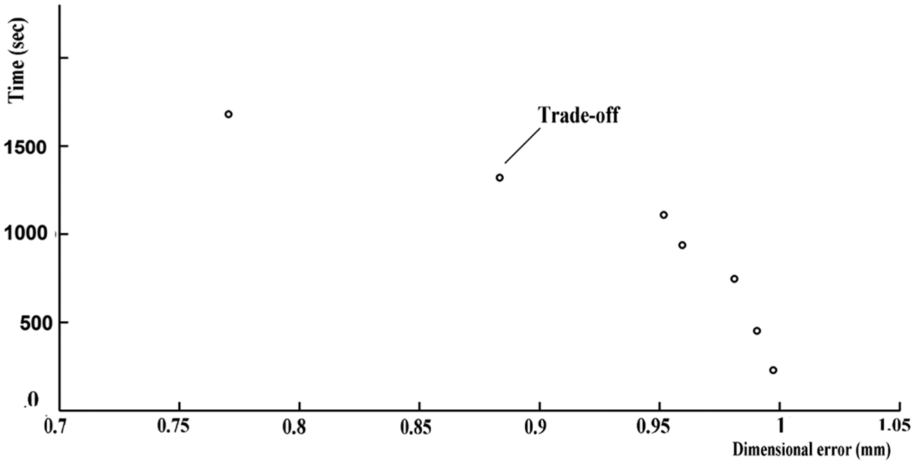
Optimal Pareto front of DE versus FT.
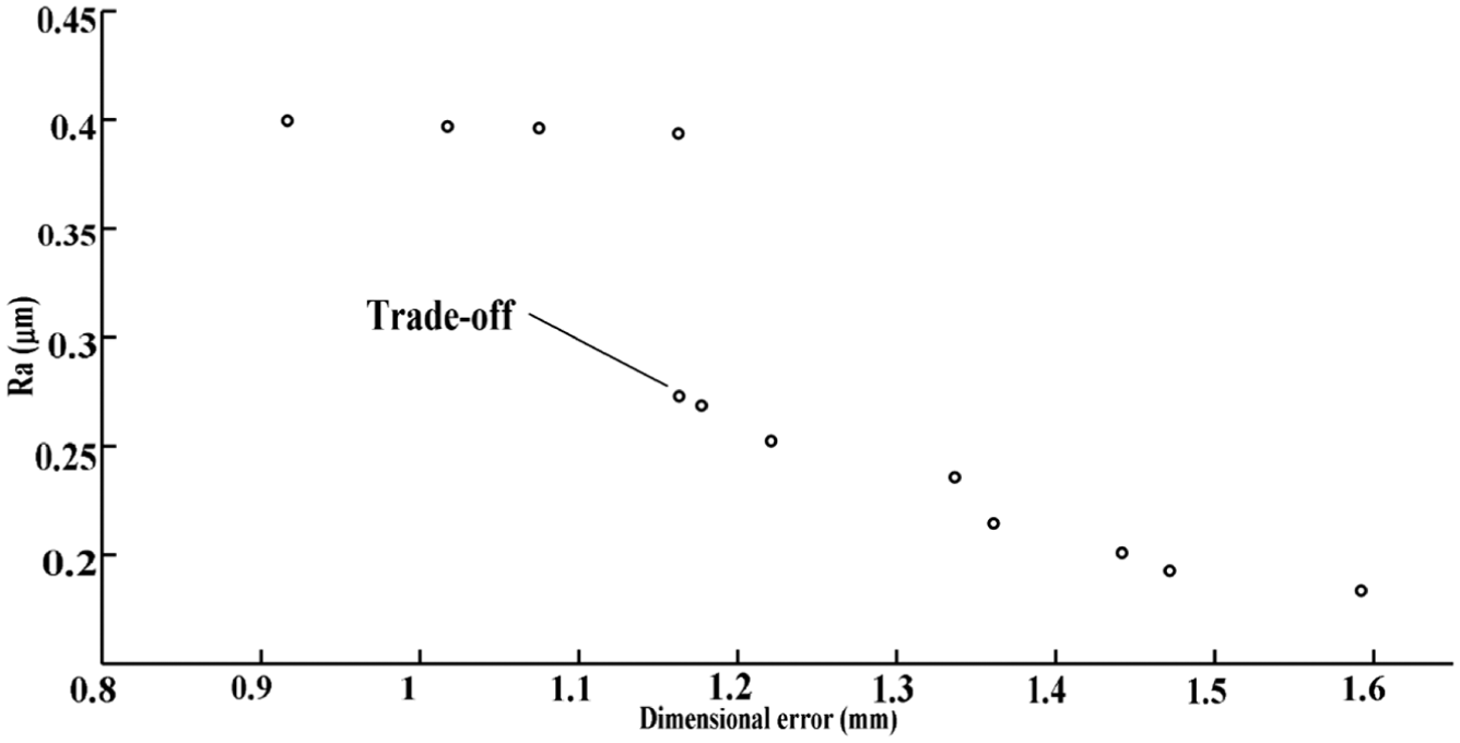
Optimal Pareto front of DE versus Ra.
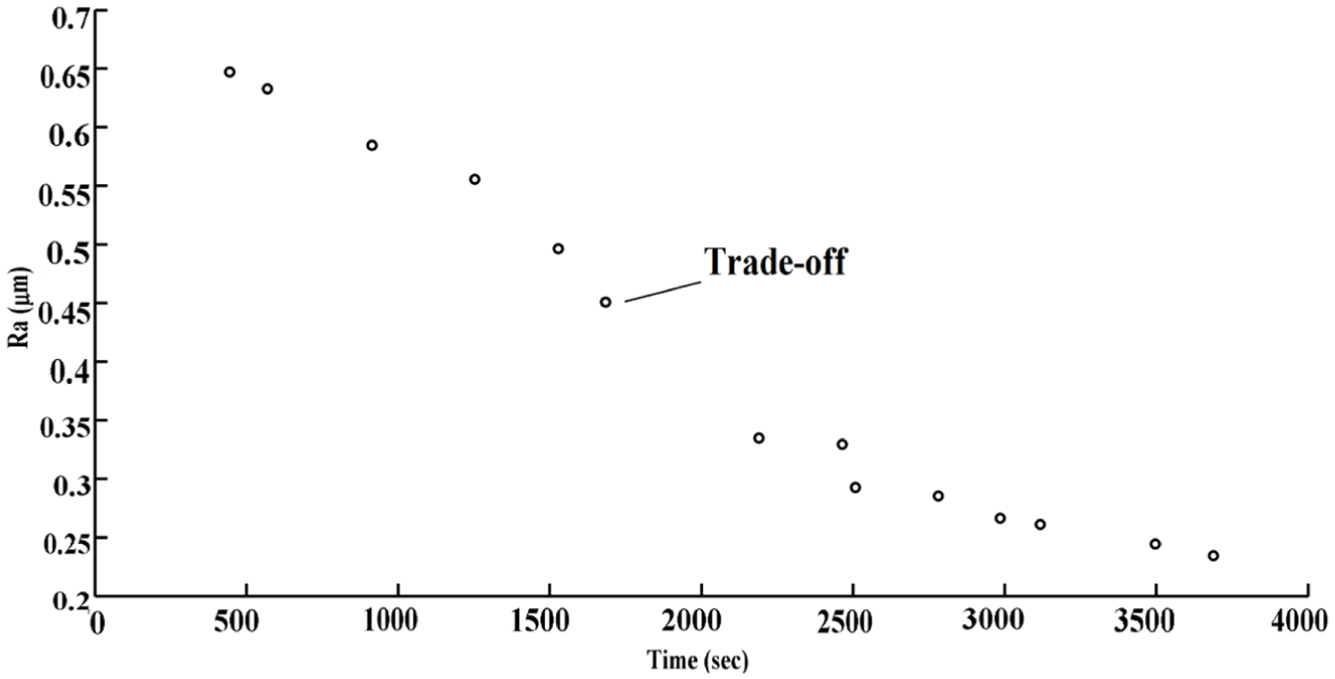
Optimal Pareto front of FT versus Ra.
Three-objective optimization
It can be concluded from the previous section that the optimization of each pair of objective functions leads to non-optimality of the third objective function. This section deals with the concurrent optimization of all the objective functions using the Multi objective uniform diversity genetic algorithm (MUGA). Figure 14 shows the Pareto front obtained from three-objective optimization in the space of the objective functions of DE, FT and surface quality. To select the tradeoff point, all the points were mapped in the (0-1) normal space. Then, the point with the shortest distance from the origin was considered the tradeoff point. Figures 15–17 show the Pareto points in the two-by-two space of the objective functions. Additionally, Table 5 gives the design variables and the corresponding optimal values of the objective functions of that tradeoff point.Table 6 shows the minimum, maximum, and optimal values of the objective functions based on the data in Tables 3 and 5.
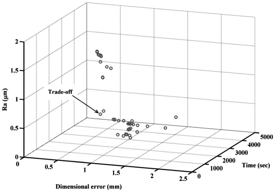
Pareto front obtained from three-objective optimization.
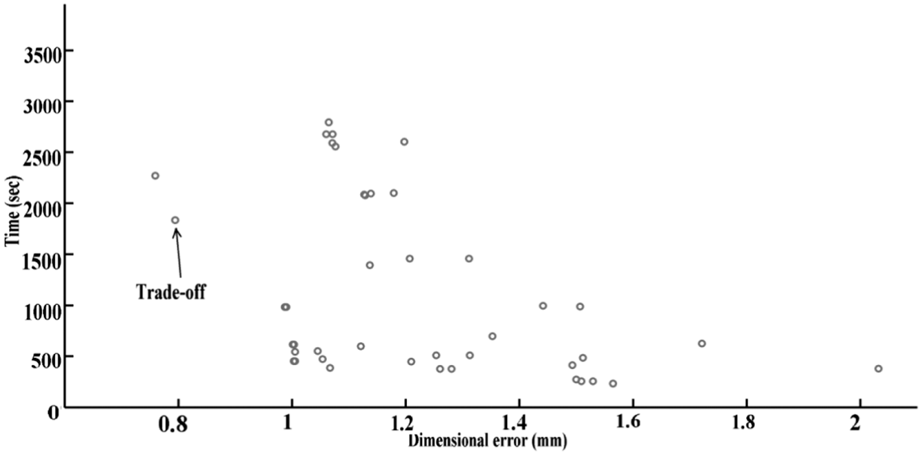
Pareto front of optimum design points on the plane of DE and FT.
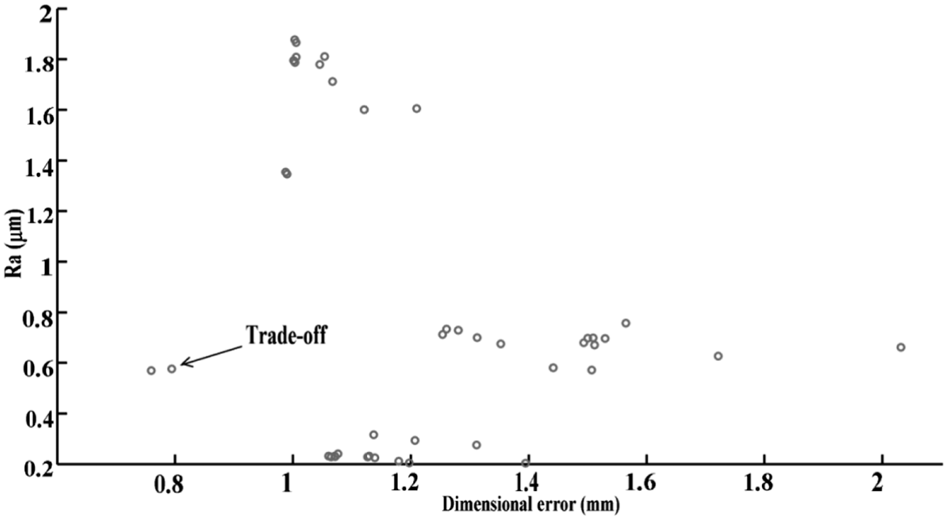
Pareto front of optimum design points on the plane of DE and Ra.
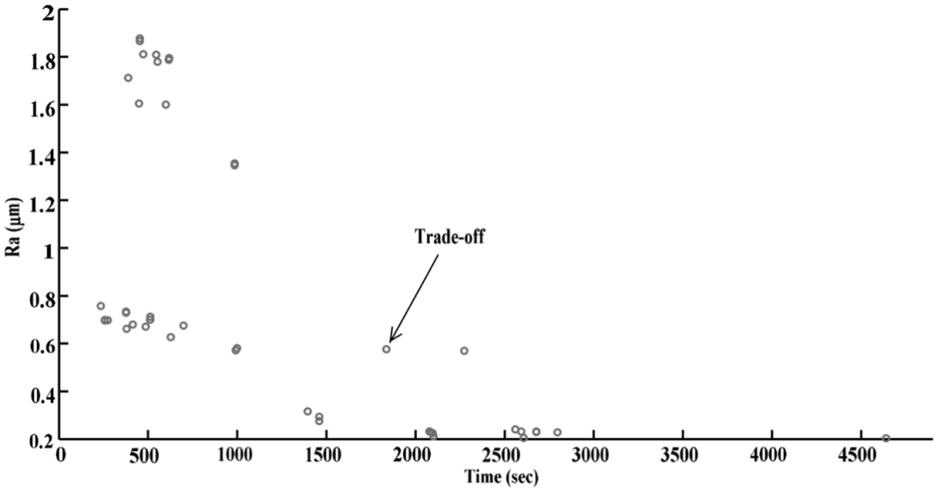
Pareto front of optimum design points on the plane of FT and Ra.
Minimum, maximum, and optimal values of the objective functions.
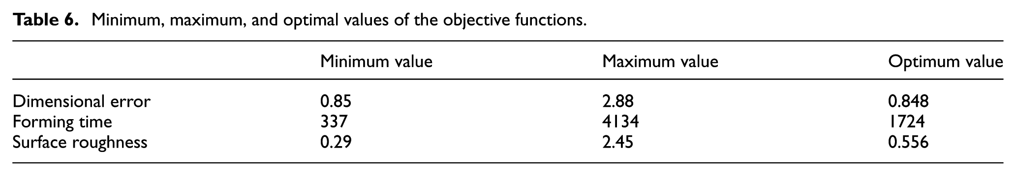
It is evident from Table 6 that the optimal value of DE is 0.848 mm, which is very close to the minimum DE (0.85 mm) observed in the experiments. In addition, the optimal value of 1724 s was obtained for FT in optimization which is acceptable when compared with the maximum FT (4134 s). Finally, the optimal value of roughness was 0.56 µm, indicating a favorable surface quality.
It is worth noting that the design variables pertinent to the tradeoff point approximately coincided with the data obtained from Experiment No. 5. This confirms the accuracy of both proposed models and the optimization process. As shown in Table 5, the tradeoff point of the objective functions under study is relatively superior to the results obtained from both single- and two-objective optimizations.
Conclusion
The manufacture of parts with high dimensional accuracy and proper quality surface at the shortest time is an important consideration in the commercialization of the SPIF process. Thus, the present study proposed a method for appropriately selecting forming parameters to minimize both DE and surface roughness at the shortest possible manufacturing time. This was accomplished by conducting experiments, developing predictive models, and performing multi-objective optimization. First, the CCD was used to study the effect of forming parameters (i.e. tool diameter, step depth, sheet thickness, and feed rate) on responses (namely, DE, FT, and surface roughness). Then, the GMDH and data obtained from DOE methods were employed to develop predictive mathematical models of the design variables.
After model accuracy evaluation by studying R2 values, single- and multi-objective optimizations were performed using the GA. The results of single-objective optimization evidently show the contradictory effects of design variables on objective functions. For instance, the lowest surface roughness occurred when the tool had the largest diameter, while the lowest level of DE occurred at the smallest tool diameter. In addition, the shortest FT was observed at the highest step depth and the highest values of feeding rate, whereas such an arrangement caused the highest degree of surface roughness. Also, simultaneous optimization of pairs of objective functions led to the degradation of the third objective function. Therefore, three-objective optimization was conducted to simultaneously optimize all the three objective functions, and the Pareto optimal front was obtained. The results indicate that the design variables of the tradeoff point correspond to the values obtained from Experiment No. 5, showing efficiency and accuracy of the models and the optimization process. In that arrangement, geometrical error was 0.79 mm, surface roughness was 0.57 µm, and FT was 1836 s, which are relatively better than those obtained from single- and two-objective optimizations. Considering the priorities of the objective functions, it is however possible for the designer to set appropriate process parameters from the results of this study.
Footnotes
Declaration of conflicting interests
The author(s) declared no potential conflicts of interest with respect to the research, authorship, and/or publication of this article.
Funding
The author(s) received no financial support for the research, authorship, and/or publication of this article.