Modified weighted standard deviation index for adequately interpreting a supplier’s lognormal process capability

Abstract

The process capability index has become an efficient tool for measuring a supplier’s process performance. $C_{\mathrm{pk}}(\mathrm{WSD})$ is one popularly used index for assessing non-normal process capability when the process violates the normality assumption. Unfortunately, this index cannot accurately reflect the process yield, so it may produce a serious result if the practitioner compares the calculated $C_{\mathrm{pk}}(\mathrm{WSD})$ value with the capability requirement to determine whether the process meets that requirement. Hence, this study modifies $C_{\mathrm{pk}}(\mathrm{WSD})$ to provide an adequate measure of lognormal process capability. In addition, an estimator of this modified index is also provided. Simulations show that the bias of this estimator is slight, and the coverage probability of capability testing is close to the nominal confidence. This means that our proposed method is adaptable for use.

Introduction

Today, increasing numbers of enterprises outsource the procurement of services or products from an outside supplier in order to cut costs. ¹ One of the biggest reasons why both small businesses and larger companies outsource is that outsourcing cuts the cost of hiring and training employees while still fulfilling labor needs. In this manner, a business allocates tasks to its outsourcing partner, which shares the workload of the employees of their own businesses. This can allow the businesses to develop their internal task force and use them more efficiently.

In short, firms utilize outsourcing as a strategic tool to leverage globally dispersed resources in order to focus on their core competencies and improve efficiency in this increasingly competitive business environment. ² However, it must be noted that the more the firms rely on outsourcing, the more they depend on their suppliers, and the more important it is to manage and develop suppliers in order to achieve and maximize the benefits of outsourcing. ² Hence, a business’ success is highly dependent on its interactions with suppliers. As noted by Wu et al., ³ a suitable supplier can substantially decrease production lead time, reduce purchasing costs, strengthen corporate competitiveness, and increase customer satisfaction. Obviously, an effective method for solving the supplier selection problem is essential to a business. An important consideration for a manufacturer is how to select, evaluate, observe, and finally create a cooperative relationship with existing or new suppliers. ⁴ Supplier selection has increasingly been regarded as one of the most important strategies in the globalization era. ⁵

In past years, various criteria for selecting better suppliers have been investigated. Dickson ⁶ concluded that quality and delivery are two of the most demanded items for component manufacturers. Moreover, Weber et al. ⁷ considered quality as having “extreme importance” and delivery as having “considerable importance” to the manufacturers. Furthermore, Pearson and Ellram ⁸ surveyed 210 members of the National Association of Purchasing Management and indicated that quality is the most important criterion for selecting a supplier. Recently, Olhager and Selldin ⁹ investigated 128 samples of Swedish manufacturing firms and concluded that many aspects are important when companies choose supply chain partners but quality is the most important criterion. In summary, quality is regarded as the most fundamental factor for supplier selection.

However, the basic step for processing supplier selection is accurately evaluating the supplier’s performance to enable a determination of the list of qualified suppliers. The principal purpose of supplier evaluation is to ensure that a portfolio of best-in-class suppliers is available for use. ¹⁰ Supplier evaluation is a process applied to current suppliers in order to measure and monitor their performance for the purposes of mitigating risk, reducing costs, and driving continuous improvement. ¹¹

Since accurately evaluating a supplier’s performance is important, the principal purpose of this study is to build a practical procedure to measure accurately a supplier’s process performance in terms of quality, the primary criterion for supplier selection. Among various quality assurance activities, process capability indices (PCIs) are widely used to interpret process capability because it is straightforward and easy to use. Using PCIs, a quality engineer can trace and improve a poor process, and a downstream manufacturer can efficiently assess his supplier’s process performance to ensure reliable decision-making on whether to purchase goods from his supplier.

The book by Kotz and Lovelace ¹² provided a complete illustration of the developing history of PCIs. Kotz and Johnson ¹³ reviewed approximately 170 important studies of PCI and conducted a clear and penetrating analysis of them. Spiring et al. ¹⁴ reviewed related papers published in 1992–2002 and categorized them systematically. Wu et al. ¹⁵ discussed the relationships of quality assurance and some major PCIs in relation to four aspects, namely, process consistency, process relative departures, process yield, and expected relative loss. In addition to the review paper above, see literature^16–22 for more discussion of PCIs.

Among various PCIs, the index $C_{\mathrm{pk}}$ ²³ remains the most widely used because it can provide bounds on process yield for normally distributed processes; ²⁴ that is, 2Φ (3 C_pk) − 1 ≤ yield% < Φ (3 C_pk), ²⁵ where $\Phi (.)$ is the cumulative distribution function of the standard normal distribution. However, processes are often non-normal in real-world applications. For non-normal processes, considerable evidence has indicated that $C_{\mathrm{pk}}$ will mislead managers into making incorrect decisions.

Because applying $C_{\mathrm{pk}}$ to assess non-normal process capability can lead to inappropriate decisions, approaches for assisting the use of PCIs for non-normal populations have been developed rapidly in past years. ²⁴ One popularly used method was proposed by Chang et al. ²⁶ They provide an index, $C_{\mathrm{pk}}(\mathrm{WSD})$ , that adjusts $C_{\mathrm{pk}}$ in accordance with the degree of skewness of the underlying population using different factors in computing the deviations above and below the process mean. ²⁶

The index $C_{\mathrm{pk}}(\mathrm{WSD})$ provides a calculation for non-normal process capability, but this calculated value can result in a serious bias relative to actual yield. To overcome this drawback, this study modifies $C_{\mathrm{pk}}(\mathrm{WSD})$ to obtain a suitable evaluation of non-normal process capability. The lognormal distribution is considered as the process distribution, and similar to Liao et al., ²⁴ the curve fitting approach is used as the major technique for achieving our goal. The reasons for which we select index $C_{\mathrm{pk}}(\mathrm{WSD})$ as an object for modification are as follows: (1) index $C_{\mathrm{pk}}(\mathrm{WSD})$ is one of the well-known indices for assessing non-normal process capability and (2) the study of Chang et al. ²⁶ showed that $C_{\mathrm{pk}}(\mathrm{WSD})$ performs better than another index $C_{\mathrm{pk}}(\mathrm{WV})$ ²⁷ in assessing lognormal process capability. In addition, the study of Wu and Swain ²⁷ showed that $C_{\mathrm{pk}}(\mathrm{WV})$ performs better than the other well-known index, $C_{\mathrm{jkp}}$ , ²⁸ and Clements’ method, ²⁹ a method designed for assessing non-normal process capability, in assessing lognormal process capability. Since index $C_{\mathrm{pk}}(\mathrm{WSD})$ has better performance than several well-known indices, we choose it for modification.

The remainder of this article is organized as follows. Section “Weighted standard deviation index” introduces $C_{\mathrm{pk}}(\mathrm{WSD})$ . Section “Modified weighted standard deviation index” illustrates how to apply curve fitting techniques to obtain a correction factor $b\prime$ for $C_{\mathrm{pk}}(\mathrm{WSD})$ for lognormal distributed processes. In this manner, the modified index $C_{\mathrm{pk}}^{\prime }(\mathrm{WSD})$ can interpret lognormal process capability more suitably than $C_{\mathrm{pk}}(\mathrm{WSD})$ . Section “Point estimator for the modified index” provides an estimator ${\tilde{C}}_{\mathrm{pk}}^{\prime }(\mathrm{WSD})$ for estimating $C_{\mathrm{pk}}^{\prime }(\mathrm{WSD})$ . For capability testing purposes, section “Confidence interval for testing capability” proposes a procedure based on standard bootstrapping to derive the lower confidence interval bound for $C_{\mathrm{pk}}^{\prime }(\mathrm{WSD})$ . Section “An example” is an example for examining the applicability of our approach. Some conclusions are drawn in section “Conclusion.”

Weighted standard deviation index

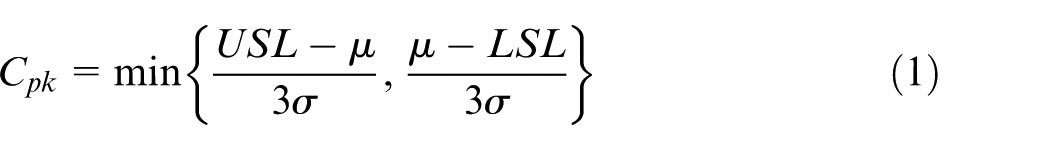
For normally distributed processes, the most widely used index $C_{\mathrm{pk}}$ is defined explicitly as follows

$$C_{\mathrm{pk}}=\min \{\frac{\mathrm{USL}-\mu }{3\sigma },\frac{\mu -\mathrm{LSL}}{3\sigma }\}$$

(1)

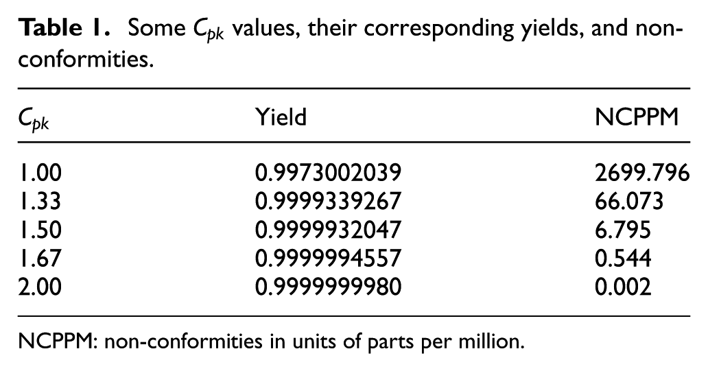
where $\mu$ is the process mean, $\sigma$ is the process standard deviation, and $\mathrm{USL}$ and $\mathrm{LSL}$ are the upper specification and lower specification limits, respectively. Table 1 lists five $C_{\mathrm{pk}}$ values, their corresponding yields, and non-conformities in units of parts per million (NCPPM), according to the following formula: 2Φ (3 C_pk) − 1 = yield%. A quality engineer can obtain the process yield or NCPPM based on a given $C_{\mathrm{pk}}$ value.

Table 1.

Some $C_{\mathrm{pk}}$ values, their corresponding yields, and non-conformities.

$C_{\mathrm{pk}}$	Yield	NCPPM
1.00	0.9973002039	2699.796
1.33	0.9999339267	66.073
1.50	0.9999932047	6.795
1.67	0.9999994557	0.544
2.00	0.9999999980	0.002

NCPPM: non-conformities in units of parts per million.

However, many process distributions violate the normality assumption. In the past, many approaches had been developed for assessing the capabilities of non-normal populations. Chang et al. ²⁶ classified these approaches. As mentioned in the works by Chang et al. ²⁶ and Pearn and Kotz, ³⁰ the first category involves the use of data transformation techniques. The second category involves the replacement of the unknown process distribution by an empirical distribution or by a known three- or four-parameter distribution. The third category involves a modification of the standard definition of PCIs in order to increase their robustness. The fourth category involves the use of heuristic arguments to develop new indices.

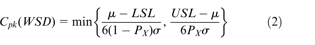
Among the methods mentioned above, a heuristic index of $C_{\mathrm{pk}}$ , namely, $C_{\mathrm{pk}}(\mathrm{WSD})$ , is the most well-known for assessing non-normal process capabilities. Suppose that $X$ is the quality characteristic. Chang et al. ²⁶ used the weighted standard deviation (WSD) method to adjust $C_{\mathrm{pk}}$ to be $C_{\mathrm{pk}}(\mathrm{WSD})$ , defined as follows

$$C_{\mathrm{pk}}(\mathrm{WSD})=\min \{\frac{\mu -\mathrm{LSL}}{6(1-P_X)\sigma },\frac{\mathrm{USL}-\mu }{6P_X\sigma }\}$$

(2)

where $P_X=P(X<\mu )$ . If the population is symmetric, then $P_X$ is equal to $1-P_X$ , and $C_{\mathrm{pk}}(\mathrm{WSD})$ reduces to $C_{\mathrm{pk}}$ . ²⁶

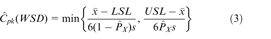
Generally, we cannot obtain overall observations of quality characteristics; therefore, we need to drop samples from a stable process to estimate $C_{\mathrm{pk}}(\mathrm{WSD})$ . Suppose that the sample observations are $\{x_1,x_2,\dots ,x_n\}$ , where $n$ is the sample size. Chang et al. ²⁶ proposed the following estimator

$${\hat{C}}_{\mathrm{pk}}(\mathrm{WSD})=\min \{\frac{\overline{x}-\mathrm{LSL}}{6(1-{\hat{P}}_X)s},\frac{\mathrm{USL}-\overline{x}}{6{\hat{P}}_{X}s}\}$$

(3)

where $\overline{x}=\sum _{i=1}^n{x}_i/n$ , $s=[\sum _{i=1}^n{(x_i-\overline{x})}^2/(n-1){]}^{1/2}$ , ${\hat{P}}_X=\sum _{i=1}^{n}I(\overline{x}-x_i)/n$ , $I(\overline{x}-x_i)=1$ , if $\overline{x}\ge x_i$ , and $I(\overline{x}-x_i)=0$ , if $\overline{x}<x_i$ .

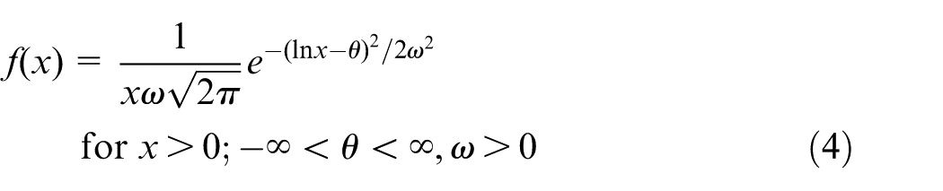
This study considers a lognormal process distribution. As noted by Limpert et al., ³¹ many measurements show a more or less skewed distribution. Skewed distributions are particularly common when mean values are low, variances are large, and values cannot be negative. Such skewed distributions often fit the lognormal distribution closely. ³¹ Moreover, Huang et al. ³² indicated that observed quality data often follow a positive skewed distribution, such as the lognormal distribution, in many real-world applications. Therefore, it is worthwhile to discuss lognormal process capability assessment in this study. If $X$ follows a lognormal distribution, the probability density function (PDF) of $X$ can be expressed as follows

$$f(x)=\frac{1}{x\omega \sqrt{2\pi }}{e}^{-{(\ln x-\theta )}^2/2{\omega }^2}\mathrm{for}x>0;-\infty <\theta <\infty ,\omega >0$$

(4)

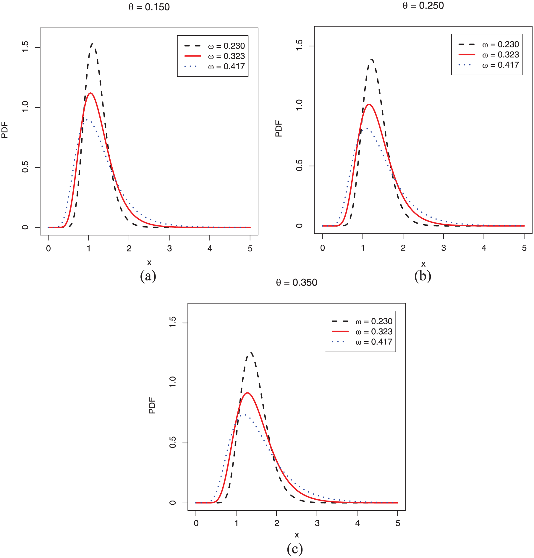
where $\theta$ is the location parameter and $\omega$ is the scale parameter. Figure 1(a)–(c) shows plots of the PDFs of the lognormal distribution for θ = 0.15, 0.25, and 0.35 with ω = 0.230, 0.323, and 0.417. These figures show that if $\omega$ increases, then the plot of the PDF becomes more skew.

Figure 1.

Plots of the PDF of lognormal distributions with (a) θ = 0.150 and various ω, (b) θ = 0.250 and various ω, and (c) θ = 0.350 and various ω.

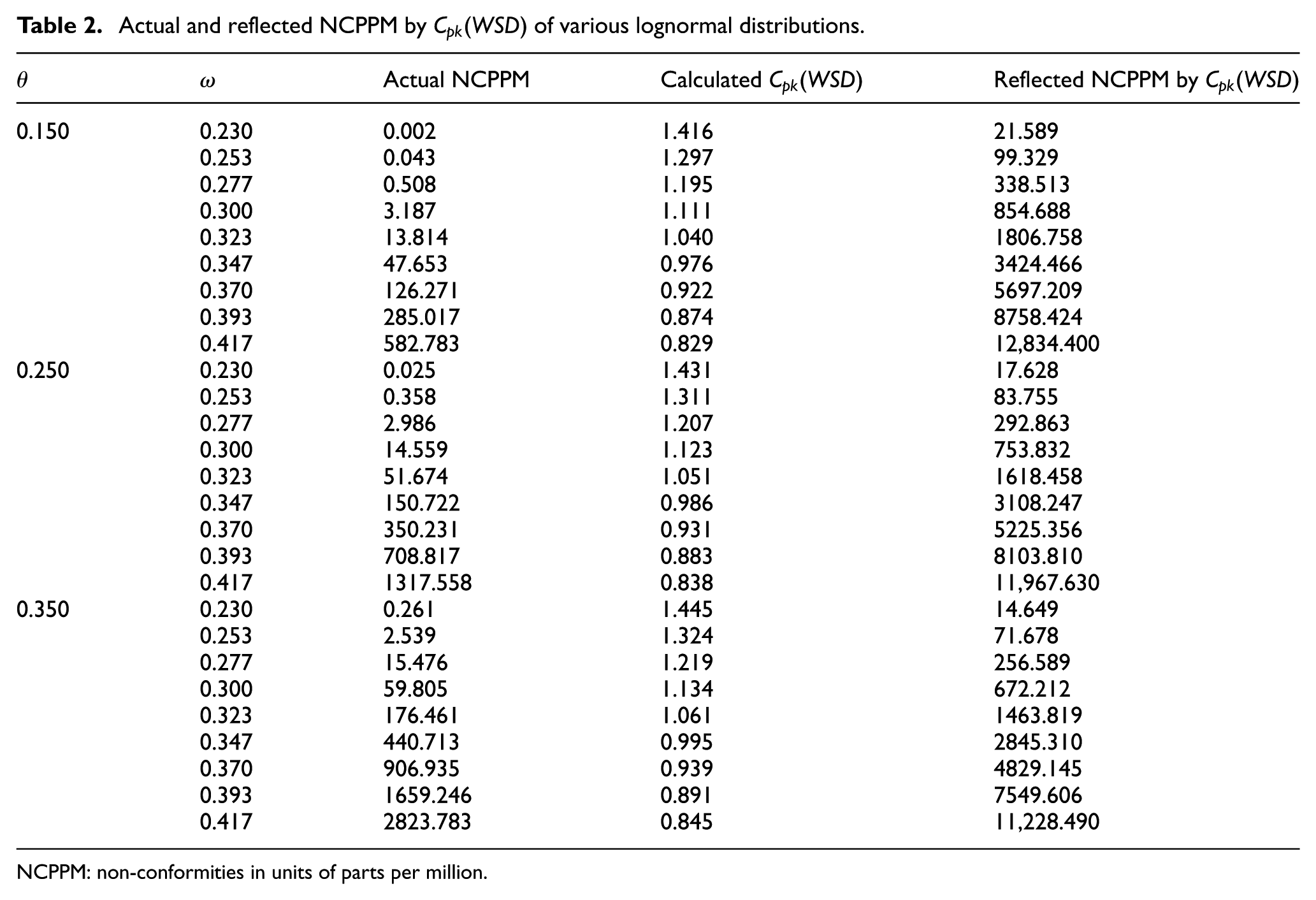
To show that $C_{\mathrm{pk}}(\mathrm{WSD})$ results in a serious bias relative to actual yield, we set θ = 0.15, 0.25, and 0.35 and ω = 0.230, 0.253, 0.277, 0.300, 0.323, 0.347, 0.370, 0.393, and 0.417 to calculate the actual values of NCPPM with the given specification limits LSL = 0.12 and USL = 4.5. Notably, the parameters, $\theta$ and $\omega$ , that we consider here can limit the actual NCPPM to be within 0.001 and 3.000 because the NCPPM values of processes for capability analysis are often in this scope (see Table 1). Therefore, a large NCPPM condition and an extremely small NCPPM condition are both excluded in our discussion. On the basis of these distributions, we also calculate the values of $C_{\mathrm{pk}}(\mathrm{WSD})$ via equation (2) and derive the corresponding NCPPMs of these values. All the results are summarized in Table 2. Notably, the “reflected NCPPM by $C_{\mathrm{pk}}(\mathrm{WSD})$ ” is obtained by ${10}^6\times (2-2\Phi )(3C_{\mathrm{pk}}(\mathrm{WSD}))$ .

Table 2.

Actual and reflected NCPPM by $C_{\mathrm{pk}}(\mathrm{WSD})$ of various lognormal distributions.

$\theta$	$\omega$	Actual NCPPM	Calculated $C_{\mathrm{pk}}(\mathrm{WSD})$	Reflected NCPPM by $C_{\mathrm{pk}}(\mathrm{WSD})$
0.150	0.230	0.002	1.416	21.589
	0.253	0.043	1.297	99.329
	0.277	0.508	1.195	338.513
	0.300	3.187	1.111	854.688
	0.323	13.814	1.040	1806.758
	0.347	47.653	0.976	3424.466
	0.370	126.271	0.922	5697.209
	0.393	285.017	0.874	8758.424
	0.417	582.783	0.829	12,834.400
0.250	0.230	0.025	1.431	17.628
	0.253	0.358	1.311	83.755
	0.277	2.986	1.207	292.863
	0.300	14.559	1.123	753.832
	0.323	51.674	1.051	1618.458
	0.347	150.722	0.986	3108.247
	0.370	350.231	0.931	5225.356
	0.393	708.817	0.883	8103.810
	0.417	1317.558	0.838	11,967.630
0.350	0.230	0.261	1.445	14.649
	0.253	2.539	1.324	71.678
	0.277	15.476	1.219	256.589
	0.300	59.805	1.134	672.212
	0.323	176.461	1.061	1463.819
	0.347	440.713	0.995	2845.310
	0.370	906.935	0.939	4829.145
	0.393	1659.246	0.891	7549.606
	0.417	2823.783	0.845	11,228.490

NCPPM: non-conformities in units of parts per million.

Table 2 indicates that $C_{\mathrm{pk}}(\mathrm{WSD})$ results in serious bias in reflecting the actual NCPPM. This underestimates the process performance. In current practice, a process is termed “Inadequate” if $C_{\mathrm{pk}}<1.00$ , “Marginally Capable” if $1.00\le C_{\mathrm{pk}}<1.33$ , “Satisfactory” if $1.33\le C_{\mathrm{pk}}<1.50$ , “Excellent” if $1.50\le C_{\mathrm{pk}}<2.00$ , and “Super” if $C_{\mathrm{pk}}\ge 2.00$ . ³³ If a process satisfies the normality assumption, then the process can be graded by its $C_{\mathrm{pk}}$ value. For instance, if the $C_{\mathrm{pk}}$ value is 1.40, then the process is categorized as Satisfactory. However, the process is often non-normal, and then, we can just use $C_{\mathrm{pk}}(\mathrm{WSD})$ instead of $C_{\mathrm{pk}}$ to assess the process capability. In current use, the decision rule for determining the process performance based on $C_{\mathrm{pk}}(\mathrm{WSD})$ is the same as that based on $C_{\mathrm{pk}}$ . For instance, if the calculated $C_{\mathrm{pk}}(\mathrm{WSD})$ value is also 1.40, then the process is also categorized as Satisfactory.

Therefore, we consider the case in which θ = 0.150 and ω = 0.300 to explain why $C_{\mathrm{pk}}(\mathrm{WSD})$ underestimates the process performance. On the basis of the preset $\theta$ and $\omega$ parameters, we can determine that the proportion outside the specification limits (USL = 4.50 and LSL = 0.12) is $3.187\times {10}^{-6}$ . This means that the NCPPM is 3.187. If a process’ NCPPM is 3.187, then the process, according to Table 1, can be categorized as Excellent. However, by the definition of $C_{\mathrm{pk}}(\mathrm{WSD})$ , we determine that the $C_{\mathrm{pk}}(\mathrm{WSD})$ value is 1.111. Thus, the process, according to the decision rule for determining the process performance, must be categorized as Marginally Capable. Therefore, we can find that $C_{\mathrm{pk}}(\mathrm{WSD})$ underestimates the process performance as well as the process yield.

Modified weighted standard deviation index

Since $C_{\mathrm{pk}}(\mathrm{WSD})$ can significantly underestimate the process yield, this section modifies $C_{\mathrm{pk}}(\mathrm{WSD})$ by multiplying it by a correction factor $b_j$ . This reduces the bias of yield estimation and increases the reliability of decision-making in capability analysis.

Suppose that our modified WSD index $C_{\mathrm{pk}}^{\prime }(\mathrm{WSD})$ is defined as follows

$$C_{\mathrm{pk}}^{\prime }(\mathrm{WSD})=b\prime \times C_{\mathrm{pk}}(\mathrm{WSD})$$

(5)

To derive the correction factor $b_j$ , we attempt to make our modified index $C_{\mathrm{pk}}^{\prime }(\mathrm{WSD})$ as well as $C_{\mathrm{pk}}$ reflect the actual NCPPM. That is, $b\prime$ is defined such that the ratio $C_{\mathrm{pk}}^{\prime }(\mathrm{WSD})/C_{\mathrm{pk}}=(b\prime \times C_{\mathrm{pk}}(\mathrm{WSD}))/C_{\mathrm{pk}}$ is approximately unity but does not exceed 1. To achieve this goal, we calculate the values $\rho \prime =C_{\mathrm{pk}}/C_{\mathrm{pk}}(\mathrm{WSD})$ for parameters θ = 0.150, 0.175, 0.200, 0.225, 0.250, 0.275, 0.300, 0.325, and 0.350 and ω = 0.230, 0.253, 0.277, 0.300, 0.323, 0.347, 0.370, 0.393, and 0.417. As a result, a total of 81 $\rho \prime$ values are obtained.

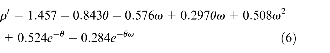
Since $\rho \prime$ is a function of $\theta$ and $\omega$ , we let $\rho \prime$ be a dependent variable, with $\theta$ and $\omega$ as the independent variables. By curve fitting

$$\rho \prime =1.457-0.843\theta -0.576\omega +0.297\theta \omega +0.508{\omega }^2+0.524e^{-\theta }-0.284e^{-\theta \omega }$$

(6)

The coefficient of determination of this model is R ²  = 99.99%; therefore, we conclude that this model is sufficient to fit those $\rho \prime$ values. Since our goal is to make $C_{\mathrm{pk}}^{\prime }(\mathrm{WSD})/C_{\mathrm{pk}}$ equal to 1, $b\prime$ is equal to $\rho \prime$ in equation (6).

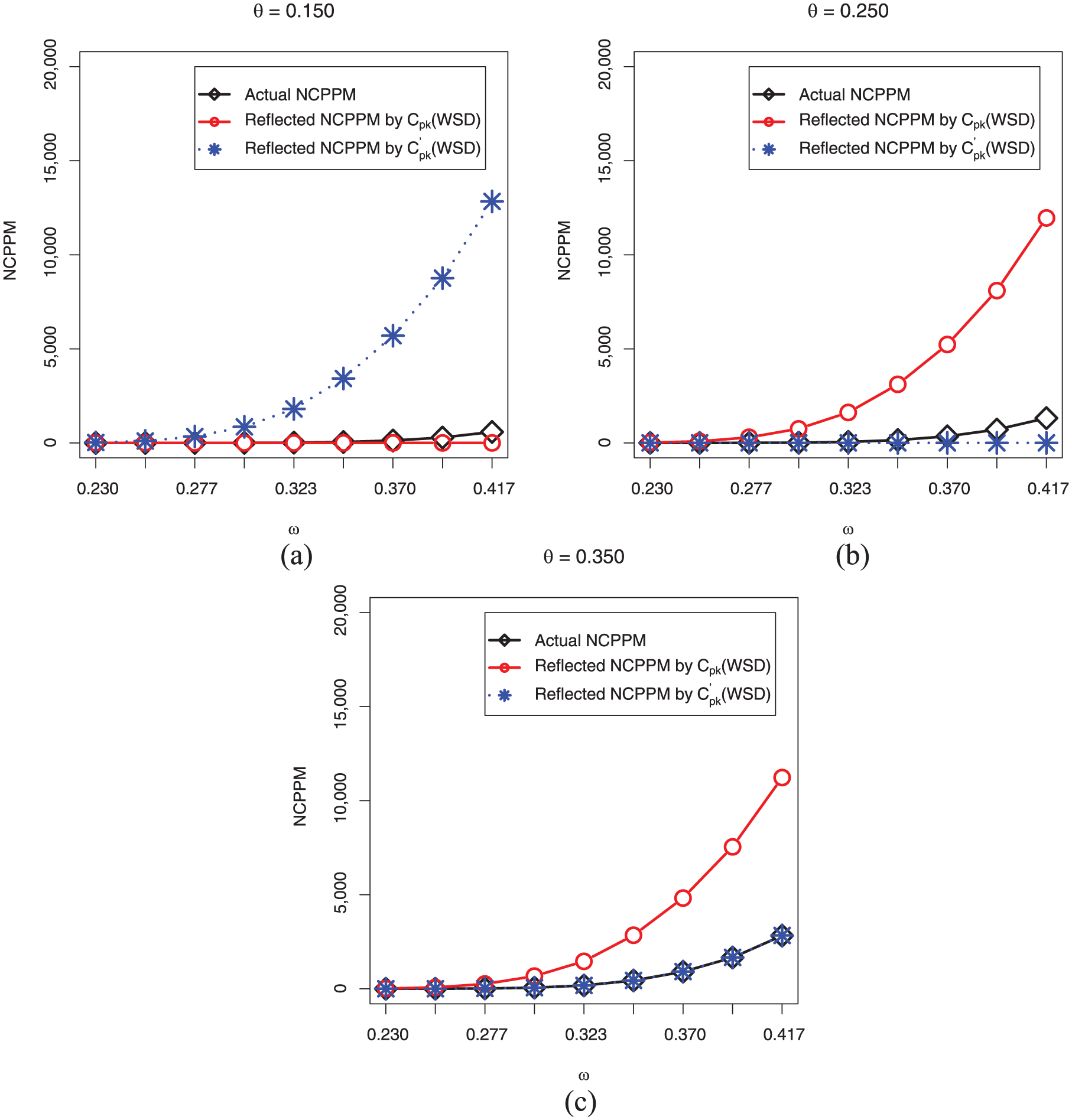
Figure 2(a)–(c) shows plots of the NCPPM and reflected NCPPM calculated using $C_{\mathrm{pk}}(\mathrm{WSD})$ and $C_{\mathrm{pk}}^{\prime }(\mathrm{WSD})$ with respect to $\omega$ for θ = 1.50, 2.50, and 3.50, separately. All figures indicate that the calculated NCPPM values derived from $C_{\mathrm{pk}}^{\prime }(\mathrm{WSD})$ are much closer to the NCPPM than those derived from $C_{\mathrm{pk}}(\mathrm{WSD})$ . Therefore, our modified index $C_{\mathrm{pk}}^{\prime }(\mathrm{WSD})$ can provide a more suitable interpretation for process capability.

Figure 2.

Actual and reflected NCPPM calculated by $C_{\mathrm{pk}}(\mathrm{WSD})$ and $C_{\mathrm{pk}}^{\prime }(\mathrm{WSD})$ for (a) θ = 0.150 and various $\omega$ , (b) θ = 0.250 and various $\omega$ , and (c) θ = 0.350 and various $\omega$ .

Point estimator for the modified index

Intuitively, we will substitute the sampling observations $\{x_1,x_2,\dots ,x_n\}$ into the formula $\hat{C}{\prime }_{\mathrm{pk}}(\mathrm{WSD})=\hat{b}\prime \times {\hat{C}}_{\mathrm{pk}}(\mathrm{WSD})$ to estimate $C_{\mathrm{pk}}^{\prime }(\mathrm{WSD})$ , where $\hat{b}\prime$ is an estimator of $b\prime$ . However, this estimator $\hat{C}{\prime }_{\mathrm{pk}}(\mathrm{WSD})$ is not an unbiased estimator of $C_{\mathrm{pk}}^{\prime }(\mathrm{WSD})$ . Therefore, this section also uses curve fitting to modify this estimator.

To show the relative bias of $\hat{C}{\prime }_{\mathrm{pk}}(\mathrm{WSD})$ , we calculate the $\hat{C}{\prime }_{\mathrm{pk}}(\mathrm{WSD})$ values for the various sample sizes n = 10(10)200 and lognormal distributions that we considered in section “Modified weighted standard deviation index”; therefore, a total of $9\times 9\times 20=1620$ combinations are considered here for discussion. Since the sampling distribution of $\hat{C}{\prime }_{\mathrm{pk}}(\mathrm{WSD})$ is complex and mathematically intractable, we calculate the $\hat{C}{\prime }_{\mathrm{pk}}(\mathrm{WSD})$ values with N = 10,000 on each combination. Then, the relative bias of each combination can be estimated by $[\mathrm{AVG}(\hat{b}\prime \times {\hat{C}}_{\mathrm{pk}}(\mathrm{WSD}))-C_{\mathrm{pk}}^{\prime }(\mathrm{WSD})]/\mathrm{AVG}(\hat{b}\prime \times {\hat{C}}_{\mathrm{pk}}(\mathrm{WSD}))=[\mathrm{AVG}(\hat{C}{\prime }_{\mathrm{pk}}(\mathrm{WSD}))-C_{\mathrm{pk}}^{\prime }(\mathrm{WSD})]/\mathrm{AVG}(\hat{C}{\prime }_{\mathrm{pk}}(\mathrm{WSD}))$ , where $AVG({{\widehat{C}}^{\prime }}_{pk}(WSD))=\sum _{i=1}^N{{\widehat{C}}^{\prime }}_{pki}(WSD)/N$ . Notably, $\hat{\theta }=2\ln (\overline{x})-(1/2)\ln ({\overline{x}}^2+s^2)$ and $\hat{\omega }=\sqrt{\ln (1+s^2/{\overline{x}}^2)}$ are used to estimate the parameters $\theta$ and $\omega$ . According to the results, the relative bias of $\hat{C}{\prime }_{\mathrm{pk}}(\mathrm{WSD})$ is somewhat significant; hence, we modify the estimator ${\hat{C}}_{\mathrm{pk}}(\mathrm{WSD})$ in the following.

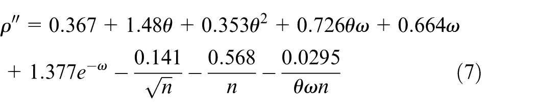
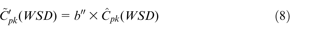
Letting $\rho ″=C_{\mathrm{pk}}^{\prime }(\mathrm{WSD})/\mathrm{AVG}({\hat{C}}_{\mathrm{pk}}(\mathrm{WSD}))$ , we can obtain a total of 1620 $\rho ″$ values for the parameters $\theta$ , $\omega$ , and $n$ . Since $\rho ″$ is a function of $\theta$ , $\omega$ , and $n$ , we let $\rho ″$ be a dependent variable, with $\theta$ , $\omega$ , and $\rho ″$ as the independent variables. Using curve fitting, we can determine that

$$\rho ″=0.367+1.48\theta +0.353{\theta }^2+0.726\theta \omega +0.664\omega +1.377e^{-\omega }-\frac{0.141}{\sqrt{n}}-\frac{0.568}{n}-\frac{0.0295}{\theta \omega n}$$

(7)

The coefficient of determination of this model is R ²  = 99.90%; therefore, we conclude that this model is sufficient to fit those $\rho ″$ values. Since our goal is to make $E(b″\times {\hat{C}}_{\mathrm{pk}}(\mathrm{WSD}))/C_{\mathrm{pk}}^{\prime }(\mathrm{WSD})$ equal to 1, where $b″$ is the correction factor for ${\hat{C}}_{\mathrm{pk}}(\mathrm{WSD})$ , $b″$ is equal to $\rho ″$ in equation (7), and the modified estimator for $C_{\mathrm{pk}}^{\prime }(\mathrm{WSD})$ is

$${\tilde{C}}_{\mathrm{pk}}^{\prime }(\mathrm{WSD})=b″\times {\hat{C}}_{\mathrm{pk}}(\mathrm{WSD})$$

(8)

Since $b″$ is unknown, we also recommend $\hat{\theta }$ and $\hat{\omega }$ for estimating $\theta$ and $\omega$ . The estimates of $b″$ and $\hat{b}″$ can be obtained in this manner.

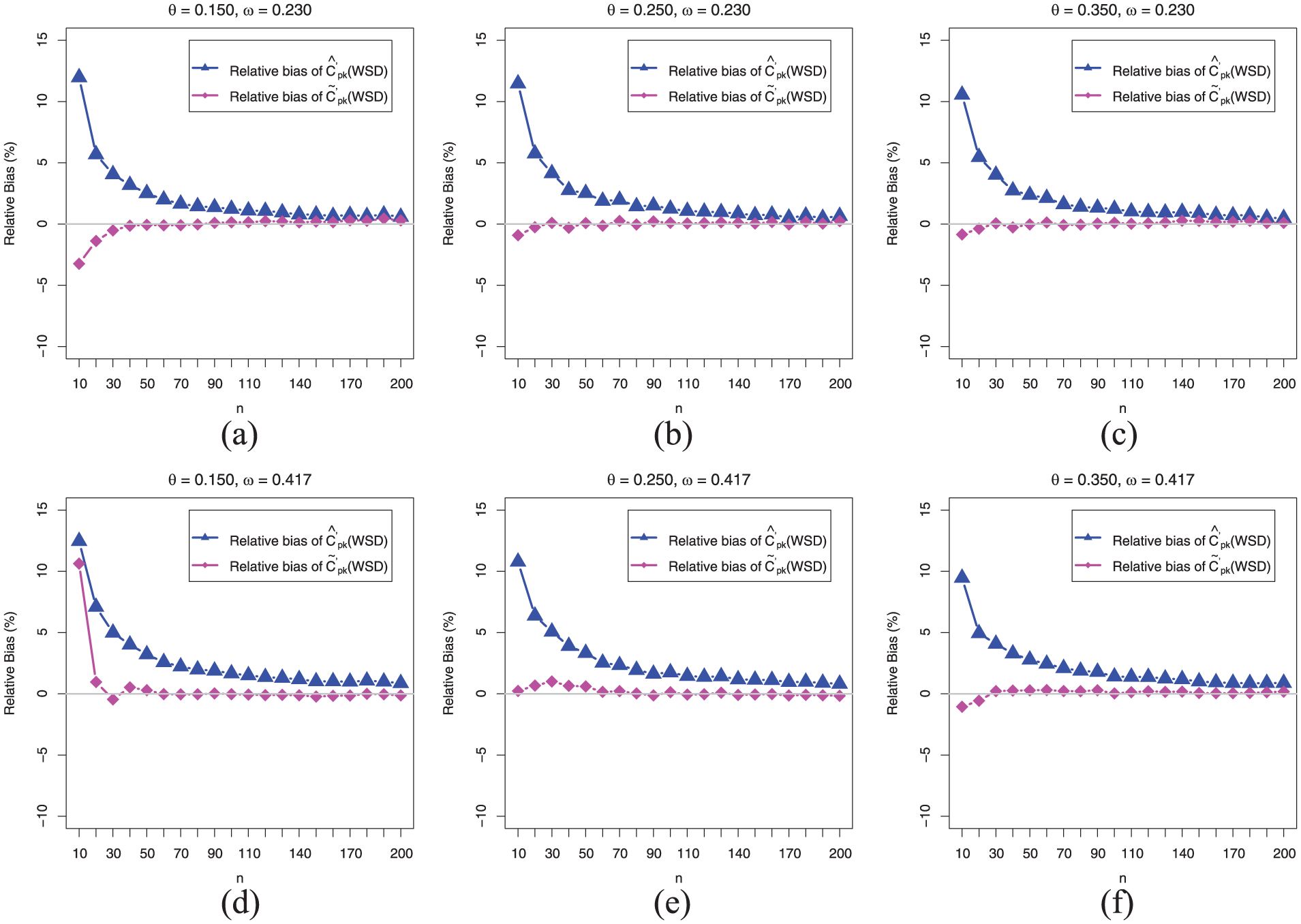
To compare ${\tilde{C}}_{\mathrm{pk}}^{\prime }(\mathrm{WSD})$ with $\hat{C}{\prime }_{\mathrm{pk}}(\mathrm{WSD})$ , we conduct Monte Carlo simulation with 10,000 replications. In these simulations, we use $\hat{b}\prime$ and $\hat{b}″$ to estimate $b\prime$ and $b″$ and apply them to ${\hat{C}}_{\mathrm{pk}}(\mathrm{WSD})$ . Then, ${\tilde{C}}_{\mathrm{pk}}^{\prime }(\mathrm{WSD})$ and $\hat{C}{\prime }_{\mathrm{pk}}(\mathrm{WSD})$ can be calculated. Figure 3(a)–(f) shows plots of the relative biases in percentage of these estimators for the parameters θ = 0.150, 0.250, and 0.350 and ω = 0.230 and 0.417. Figure 3(a)–(f) shows that the modified estimator ${\tilde{C}}_{\mathrm{pk}}^{\prime }(\mathrm{WSD})$ significantly reduces the bias in estimating $C_{\mathrm{pk}}^{\prime }(\mathrm{WSD})$ . Moreover, the absolute values of these biases are almost smaller than 0.5%. Therefore, we conclude that ${\tilde{C}}_{\mathrm{pk}}^{\prime }(\mathrm{WSD})$ is more accurate than $\hat{C}{\prime }_{\mathrm{pk}}(\mathrm{WSD})$ for estimating $C_{\mathrm{pk}}^{\prime }(\mathrm{WSD})$ .

Figure 3.

Relative biases of $\hat{C}{\prime }_{\mathrm{pk}}(\mathrm{WSD})$ and ${\tilde{C}}_{\mathrm{pk}}^{\prime }(\mathrm{WSD})$ for (a) θ = 0.150 and ω = 0.230, (b) θ = 0.250 and ω = 0.230, (c) θ = 0.350 and ω = 0.230, (d) θ = 0.150 and ω = 0.417, (e) θ = 0.250 and ω = 0.417, and (f) θ = 0.350 and ω = 0.417.

In this study, the parameters, $\theta$ and $\omega$ , and the specification limits, USL and LSL, are set before we derive the correction factors. However, our proposed correction factors are still applicable even if $\theta$ , $\omega$ , or the specification limits vary because we can find that the modified index and its estimator are both functions of $\theta$ , $\omega$ , USL, and LSL.

Confidence interval for testing capability

Suppose that the capability requirement is $c$ , which is usually set as 1.00, 1.33, 1.50, 1.67, or 2.00, as listed in Table 1. The testing hypotheses for testing process capability can be defined as $H_0:C_{\mathrm{pk}}^{\prime }(\mathrm{WSD})=c$ and $H_1:C_{\mathrm{pk}}^{\prime }(\mathrm{WSD})>c$ . ${\tilde{C}}_{\mathrm{pk}}^{\prime }(\mathrm{WSD})$ can accurately estimate $C_{\mathrm{pk}}^{\prime }(\mathrm{WSD})$ , but we cannot compare ${\tilde{C}}_{\mathrm{pk}}^{\prime }(\mathrm{WSD})$ directly to $c$ to determine whether the null hypothesis is to be rejected. In this case, we must take the sampling error into account. However, the sampling distribution of ${\tilde{C}}_{\mathrm{pk}}^{\prime }(\mathrm{WSD})$ is also complex and mathematically untraceable; therefore, this study recommends standard bootstrapping^34,35 to obtain the lower confidence interval bound $L$ for $C_{\mathrm{pk}}^{\prime }(\mathrm{WSD})$ . If $L>c$ , then we reject the null hypothesis and conclude that the process meets the capability requirement; otherwise, we cannot reject the null hypothesis, and the process cannot be determined as capable. The bootstrap procedure is described as follows:

• Step 1. Set the number of bootstrap samples $B$ .

• Step 2. Drop a random sample of size $n$ from a stable process and record the critical quality characteristic as $\{x_1,x_2,\dots ,x_n\}$ .

• Step 3. Drop a sample of size $n$ from $\{x_1,x_2,\dots ,x_n\}$ with replacement. This is a bootstrap sample $\{x_1^{*},x_2^{*},\dots ,x_n^{*}\}$ .

• Step 4. Compute ${\tilde{C}}_{\mathrm{pk}}^{\prime }(\mathrm{WSD})$ , the estimate of $C_{\mathrm{pk}}^{\prime }(\mathrm{WSD})$ , based on the data $\{x_1^{*},x_2^{*},\dots ,x_n^{*}\}$ .

• Step 5. Repeat steps 3 and 4 $B$ times, and $B$ bootstrap estimates of $C_{\mathrm{pk}}^{\prime }(\mathrm{WSD})$ , namely, $\{{\tilde{C}\prime }_{\mathrm{pk}2}^{*}(\mathrm{WSD}),{\tilde{C}\prime }_{\mathrm{pk}2}^{*}(\mathrm{WSD}),\dots ,{\tilde{C}\prime }_{\mathrm{pkB}}^{*}(\mathrm{WSD})\}$ , are obtained.

• Step 6. Compute the average value, $\mathrm{AVG}({\tilde{C}\prime }_{\mathrm{pk}}^{*}(\mathrm{WSD}))$ , and standard deviation, $\mathrm{SD}({\tilde{C}\prime }_{\mathrm{pkB}}^{*}(\mathrm{WSD}))$ , of those respective bootstrap estimates.

• Step 7. Let $\delta$ be the degree of type I error. The standard bootstrap interval is $L=\mathrm{AVG}({\tilde{C}\prime }_{\mathrm{pkB}}^{*}(\mathrm{WSD}))-Z_{\delta }\times \mathrm{SD}({\tilde{C}\prime }_{\mathrm{pkB}}^{*}(\mathrm{WSD}))$ , where $Z_{\delta }$ is the upper $100\times \delta$ percentile of a standard normal distribution.

An example

In the following, we consider the example provided by Pearn et al. ³⁶ of manufacturing thin-film transistor liquid-crystal display (TFT-LCD) products. The example assumes that the color filter is the most key component for a TFT-LCD and that the “thickness” of the color filter is the critical-to-quality (CTQ) factor. If the thickness of the color filter is not in control, then the TFT-LCD product might result in some degree of aberration. ³⁷

Suppose that a downstream manufacturer of a TFT-LCD product wants to evaluate his supplier’s process capability to be able to determine whether his company should accept the products. He decides to use process capability analysis to make further decisions; therefore, $C_{\mathrm{pk}}^{\prime }(\mathrm{WSD})$ is adopted. The process specification limits of the thickness of the specific TFT-LCD product are LSL = 10 mm and USL = 20 mm. According to his company’s requirement, the process must be at least Marginally Capable; that is, $c$ is determined as 1.00, and the statistical hypotheses are defined as $H_0:C_{\mathrm{pk}}^{\prime }(\mathrm{WSD})=1.00$ and $H_1:C_{\mathrm{pk}}^{\prime }(\mathrm{WSD})>1.00$ . If $H_0$ is rejected, then the manufacturer can accept his supplier’s products.

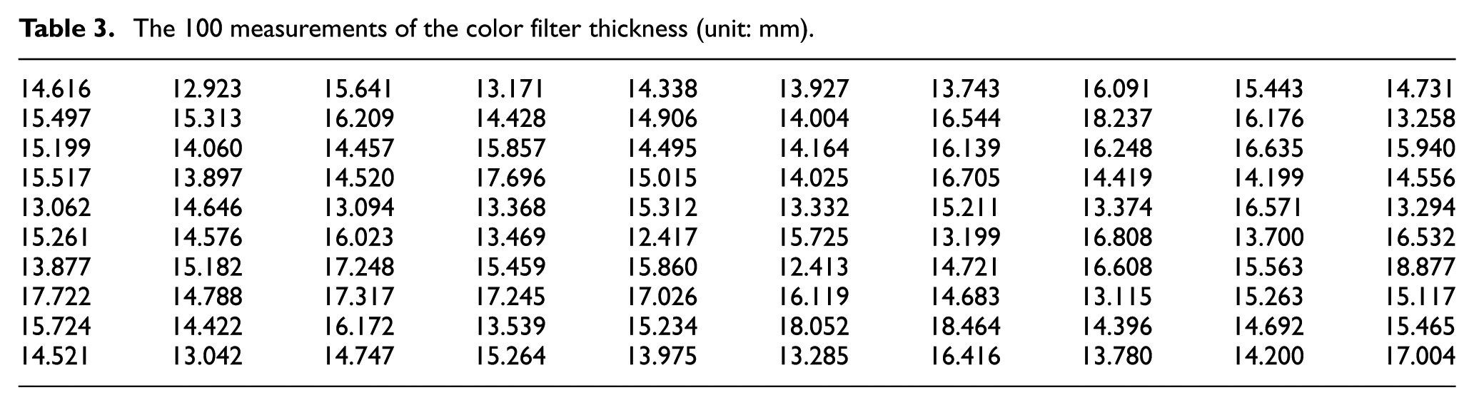
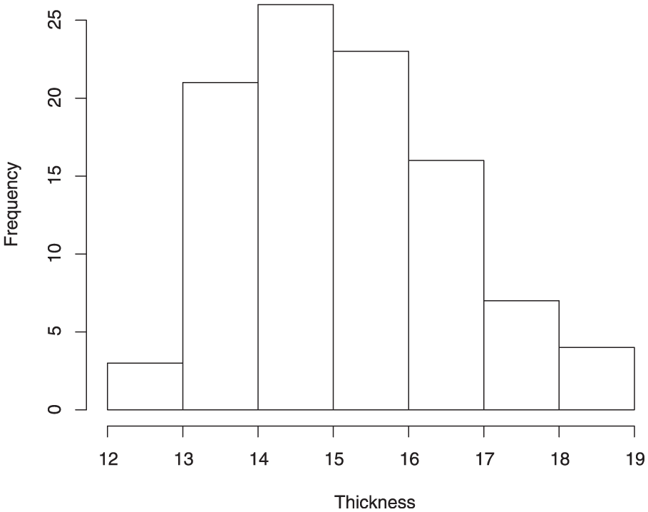
After randomly sampling products from a stable process, a batch of products with sample size n = 100 is collected (see Table 3). Figure 4 is the histogram of those quality observations. It shows that the process distribution is right-skewed, thereby enabling him to ensure that the process does not satisfy the normality assumption. In fact, past experiments indicate that the produced thickness data follow a lognormal distribution. Hence, the manufacturer uses equation (3) to obtain ${\hat{C}}_{\mathrm{pk}}(\mathrm{WSD})$ as 1.130. Since both $\theta$ and $\omega$ are unknown, he uses $\hat{\theta }=2\ln (\overline{x})-(1/2)\ln ({\overline{x}}^2+s^2)=0.407$ and $\hat{\omega }=\sqrt{\ln (1+s^2/{\overline{x}}^2)}=0.094$ to estimate them. As a result, the estimate of $b″$ can be obtained as $\hat{b}″=1.140$ . By applying $\hat{b}″$ to ${\hat{C}}_{\mathrm{pk}}(\mathrm{WSD})$ , the estimate of $C_{\mathrm{pk}}^{\prime }(\mathrm{WSD})$ is ${\tilde{C}}_{\mathrm{pk}}^{\prime }(\mathrm{WSD})=1.288$ . Since the sampling error must be considered in statistical testing, bootstrapping is adopted to evaluate the 95% confidence interval bound. On the basis of B = 2000 bootstrap samples, the 95% lower confidence interval bound is L = 1.050. Since $L>c$ , the manufacturer rejects $H_0$ and accepts the supplier’s products.

Table 3.

The 100 measurements of the color filter thickness (unit: mm).

14.616	12.923	15.641	13.171	14.338	13.927	13.743	16.091	15.443	14.731
15.497	15.313	16.209	14.428	14.906	14.004	16.544	18.237	16.176	13.258
15.199	14.060	14.457	15.857	14.495	14.164	16.139	16.248	16.635	15.940
15.517	13.897	14.520	17.696	15.015	14.025	16.705	14.419	14.199	14.556
13.062	14.646	13.094	13.368	15.312	13.332	15.211	13.374	16.571	13.294
15.261	14.576	16.023	13.469	12.417	15.725	13.199	16.808	13.700	16.532
13.877	15.182	17.248	15.459	15.860	12.413	14.721	16.608	15.563	18.877
17.722	14.788	17.317	17.245	17.026	16.119	14.683	13.115	15.263	15.117
15.724	14.422	16.172	13.539	15.234	18.052	18.464	14.396	14.692	15.465
14.521	13.042	14.747	15.264	13.975	13.285	16.416	13.780	14.200	17.004

Figure 4.

Histogram of the color filter thickness.

Practicability of the modified index

In section “An example,” we provided a TFT-LCD quality-testing example to show the usefulness of our proposed method. In our opinion, not only TFT-LCD quality but also almost lognormal distributed quality can be tested by our proposed method. Another example of lognormal quality data can be seen in evaluating the quality of engine oil in the automotive industry. Quality engineers need to measure the percent viscosity increase (PVIS) of engine oil after it has been put to the test for a specific period of time. Here, the PVIS data follow a lognormal distribution. ³² In addition, products having lognormal quality characteristics can indeed be found in many applications, such as chemical, semiconductor, cutting, drilling, grinding, and polishing processes. In these processes, the CTQ factor varies, including thickness, flatness, depth, length, width, electric current, hardness, concentration, strength, operational life, viscosity, or noise. All these might follow a lognormal distribution. The practitioner can use the chi-square goodness-of-fit test to check whether the quality characteristic of interest follows a lognormal distribution. If it passes the test, our proposed method can be applied.

In the following, we provide Monte Carlo simulations to discuss the performance of our proposed method. The major criterion for measuring the performance is coverage probability, the proportion of the time that the confidence interval contains the nominal confidence of interest. ³⁸ If the coverage probability is too large, our proposed method must be determined to be conservative, whereas if the coverage probability is too small, then our proposed method must be determined to be liberal. ³⁹

The lognormal parameters in the simulation are set as θ = 0.150, 0.175, 0.200, 0.225, 0.250, 0.275, 0.300, 0.325, and 0.350 and ω = 0.230, 0.253, 0.277, 0.300, 0.323, 0.347, 0.370, 0.393, and 0.417. The specification limits are set as LSL = 0.12 and USL = 4.5. As mentioned in section “Weighted standard deviation index,” the parameters, $\theta$ and $\omega$ , that we considered here can limit the actual NCPPM to be from 0.001 to 3000. Notably, this setting has taken almost lognormal processes into account because the actual values of the NCPPM of almost real-world manufacturing processes fall in this range.

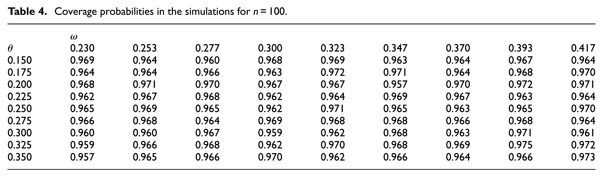
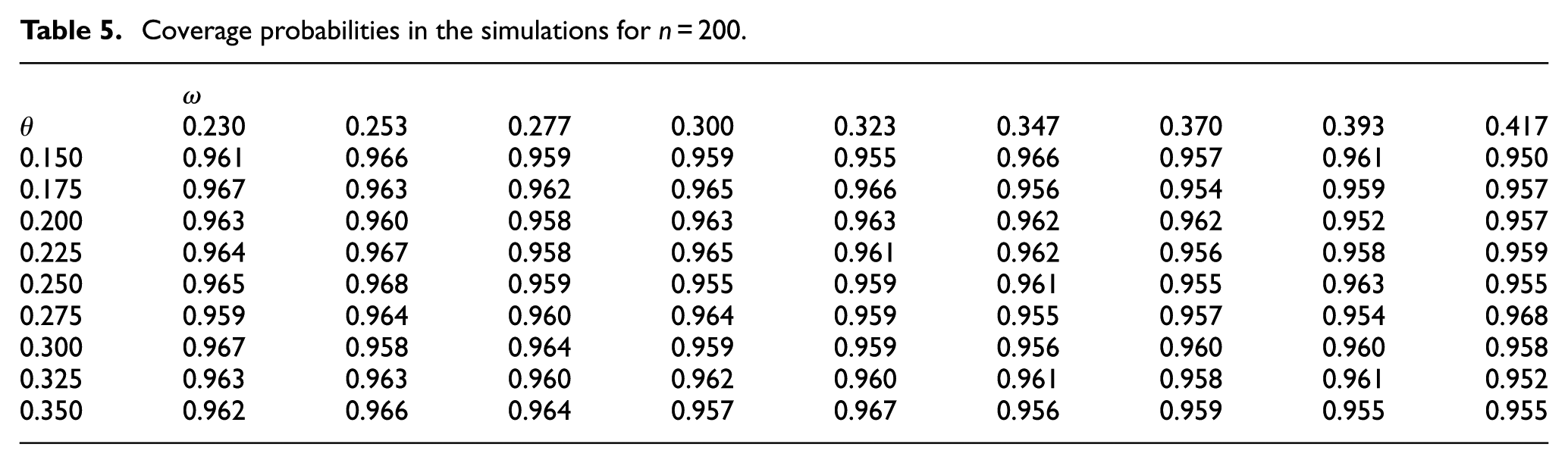
The coverage probabilities for sample sizes n = 100 and 200 after 3000 replications are conducted in the Monte Carlo simulations are listed in Tables 4 and 5, respectively. Obviously, those coverage probabilities are very close to the nominal confidence, 0.95, especially when the sample size is sufficiently large. On the basis of our simulation results, we can conclude that our proposed method is suitable for testing lognormal process capabilities.

Table 4.

Coverage probabilities in the simulations for n = 100.

	$\omega$
$\theta$	0.230	0.253	0.277	0.300	0.323	0.347	0.370	0.393	0.417
0.150	0.969	0.964	0.960	0.968	0.969	0.963	0.964	0.967	0.964
0.175	0.964	0.964	0.966	0.963	0.972	0.971	0.964	0.968	0.970
0.200	0.968	0.971	0.970	0.967	0.967	0.957	0.970	0.972	0.971
0.225	0.962	0.967	0.968	0.962	0.964	0.969	0.967	0.963	0.964
0.250	0.965	0.969	0.965	0.962	0.971	0.965	0.963	0.965	0.970
0.275	0.966	0.968	0.964	0.969	0.968	0.968	0.966	0.968	0.964
0.300	0.960	0.960	0.967	0.959	0.962	0.968	0.963	0.971	0.961
0.325	0.959	0.966	0.968	0.962	0.970	0.968	0.969	0.975	0.972
0.350	0.957	0.965	0.966	0.970	0.962	0.966	0.964	0.966	0.973

Table 5.

Coverage probabilities in the simulations for n = 200.

	$\omega$
$\theta$	0.230	0.253	0.277	0.300	0.323	0.347	0.370	0.393	0.417
0.150	0.961	0.966	0.959	0.959	0.955	0.966	0.957	0.961	0.950
0.175	0.967	0.963	0.962	0.965	0.966	0.956	0.954	0.959	0.957
0.200	0.963	0.960	0.958	0.963	0.963	0.962	0.962	0.952	0.957
0.225	0.964	0.967	0.958	0.965	0.961	0.962	0.956	0.958	0.959
0.250	0.965	0.968	0.959	0.955	0.959	0.961	0.955	0.963	0.955
0.275	0.959	0.964	0.960	0.964	0.959	0.955	0.957	0.954	0.968
0.300	0.967	0.958	0.964	0.959	0.959	0.956	0.960	0.960	0.958
0.325	0.963	0.963	0.960	0.962	0.960	0.961	0.958	0.961	0.952
0.350	0.962	0.966	0.964	0.957	0.967	0.956	0.959	0.955	0.955

Conclusion

This study considered the well-known non-normal PCI $C_{\mathrm{pk}}(\mathrm{WSD})$ to assess lognormal process capability. Although $C_{\mathrm{pk}}(\mathrm{WSD})$ can adjust $C_{\mathrm{pk}}$ in accordance with the degree of skewness, it still results in serious bias in the estimation of process yield. On the other hand, even if $C_{\mathrm{pk}}(\mathrm{WSD})$ is calculated, the practitioner cannot judge correctly whether the capability meets the requirement because it significantly underestimates the process performance.

Hence, this study used curve fitting to modify $C_{\mathrm{pk}}(\mathrm{WSD})$ to obtain a more suitable evaluation of lognormal process capability. The result shows that the modified index, $C_{\mathrm{pk}}^{\prime }(\mathrm{WSD})$ , can significantly reduce the bias in assessing the process yield. In other words, the modified index, $C_{\mathrm{pk}}^{\prime }(\mathrm{WSD})$ , can reflect actual non-conformities with more accuracy than $C_{\mathrm{pk}}(\mathrm{WSD})$ .

Moreover, an estimator ${\tilde{C}}_{\mathrm{pk}}^{\prime }(\mathrm{WSD})$ for estimating $C_{\mathrm{pk}}^{\prime }(\mathrm{WSD})$ was also derived in this study using curve fitting. Through simulations, it was shown that the relative bias of ${\tilde{C}}_{\mathrm{pk}}^{\prime }(\mathrm{WSD})$ is slight. Hence, using ${\tilde{C}}_{\mathrm{pk}}^{\prime }(\mathrm{WSD})$ to estimate $C_{\mathrm{pk}}^{\prime }(\mathrm{WSD})$ is appropriate.

This study provided a suitable estimation for measuring lognormal process capability, which can help the business manager to make reliable decisions regarding quality assurance activities. However, large NCPPM and extremely small NCPPM conditions were both excluded; hence, our proposed method might not be applicable in these cases. In the future, we can extend our approach to modify $C_{\mathrm{pk}}(\mathrm{WSD})$ to assess gamma and Weibull process capabilities, since some processes behave according to these kinds of distributions.