
Abstract
Control of temperature in large-scale manufacturing environments is not always practical or economical, introducing thermal effects including variation in ambient refractive index and thermal expansion. Thermal expansion is one of the largest contributors to measurement uncertainty; however, temperature distributions are not widely measured. Uncertainties can also be introduced in scaling to standard temperature. For more complex temperature distributions with non-linear temperature gradients, uniform scaling is unrealistic. Deformations have been measured photogrammetrically in two thermally challenging scenarios with localised heating. Extended temperature measurement has been tested with finite element analysis to assess a compensation methodology for coordinate measurement. This has been compared to commonly used uniform scaling and has outperformed this with a highly simplified finite element analysis simulation in scaling a number of coordinates at once. This work highlighted the need for focus on reproducible temperature measurement for dimensional measurement in non-standard environments.
Keywords
Introduction
The manufacture of products, particularly at the large scale, requires accurate measurement techniques. Specifications for product assembly in space and aerospace applications can be demanding and can be affected by deformation. 1 There has been great interest in measurement-assisted assembly (MAA) techniques that can improve these processes with deformation in mind.2,3 The key limitation is in the dimensional uncertainty that can be achieved.
Thermal effects are a large – often the largest – source of uncertainty in dimensional measurement.4–6 Standard metrology temperature is 20 °C, 7 and ideally, the metrology environment is temperature-controlled to achieve this. Large scale applications rarely have this luxury as it can often be impractical, and prohibitively costly to achieve in such vast volumes. Thermal gradients can be observed of several degrees vertically and horizontally. Temporally, variations of 10 °C–15 °C in 24 h could be expected in a large-volume assembly, integration and test (AIT) environment. This can significantly affect assembly variation.8,9
Many instruments for large-volume metrology are also afflicted by uncertainties due to ambient refractive index changes. Temperature is one of the main contributors to refractive index variation, 10 alongside other variables such as pressure, humidity, air composition (e.g. CO2 levels), and particulate contaminants (e.g. dust).
When measurements are made at non-standard temperatures, scaling back to 20 °C has to be performed based upon the coefficient of thermal expansion (CTE) of the material to be measured. Common materials such as aluminium alloys have significant thermal expansion of 23.4 µm m−1 °C−1.
Two major problems in thermal compensation methodologies are the temperature measurement planning and the method of scaling. Hybrid metrology was created for dimensional measurement scaling in complex, non-standard thermal environments. Temperature measurement data combined with computational simulation of thermal expansion can be used to model deformation, and subsequently transform measured three-dimensional (3D) coordinates. 11
Although being one of the most widely measured quantities, 12 temperature measurement is not comprehensively carried out in assembly environments. Laser trackers are portable coordinate measurement machines (PCMMs), which have a weather station measuring temperature at the instrument, alongside pressure and humidity. This is may be different to that which is to be measured (e.g. product or tooling structure). Temperature measurement technologies suitable for thermal compensation in AIT environments have been identified 13 and the literature reviewed in detail. 14 In many areas of engineering manufacture, there is a need to be able to understand and model thermal effects. This is particularly true for machine tools where thermal effects can affect the accuracy of manufacture.15–17
Photogrammetry is an increasingly common measurement technique in large-volume metrology. Targets are adhered to the surface of the measurand, many photographs are taken, and software can measure these targets as coordinates when referenced to scale bars. The ability to measure multiple targets makes photogrammetry ideal for the measurement of deformation. 18 Photogrammetry does not typically have a weather station like the laser tracker. The number of measured points is numerous, making target-specific scaling attractive.
The hybrid metrology method has been outlined and experimentally tested in challenging laboratory-scale photogrammetric measurements, before being compared to traditional thermal compensation methods. The main objective of this work was to highlight the most significant area to focus future research efforts in this field – temperature measurement or scaling. This further develops the work done previously in the definition of the method 19 and extends work presented at DET 2016. 20 Temperature measurement planning is an area in which there is an opportunity to create a reproducible strategy so that dimensional metrologists can better communicate the context of their results regardless of the technologies they have available for scaling. The work also helped to validate the simulation and further develop the methodology so that it can be easily used for a large number of coordinates.
Hybrid metrology thermal compensation
The hybrid metrology approach has been created to integrate thermal and dimensional measurement. Hybrid metrology refers to a methodology based upon the measurement of more than one physical quantity, combined with one or more computational processes including simulation for the scaling of dimensional measurements, as presented in 2015. 19
For thermal compensation, hybrid metrology combines multi-positional temperature logging with finite element analysis (FEA) performed on the nominal computer-aided design (CAD) model to produce a scaling transformation of dimensional coordinates. Temperature is measured more broadly, meaning that more complex, non-linear thermal expansion can be compensated.
Figure 1 provides some context as to how this methodology fits into manufacturing operations in order to provide thermal compensation to dimensional metrology. Product design specifications are provided to enable manufacturing, alongside a digital representation of the nominal product, that is, the CAD model. Components and sub-assemblies are manufactured to these specifications and used in the AIT of the product. Assembly operations are performed and dimensional inspection is carried out to ensure the assembly meets specifications. Measurements are taken on the physical product using the measurement instrumentation and the temperature sensors. In software, the coordinate measurements taken are aligned to match the coordinate system of the FEA and nearest nodes to measured targets are assigned. Temperature measurements are used to create boundary conditions to simulate within FEA the predicted thermal expansion based on the CAD data. The structural FEA produces displacement data which are used as part of a transformation on the measured coordinates to produce a simulated measurement that more realistically represents the conditions that the physical product is subjected to in the AIT environment. These data can be later used to make better decisions in assembly operations by providing more accurate measurements. One example would be to use the simulated measurement to predict tolerance stack-up throughout the assembly. In other situations where there is reconfigurable tooling, this could be adjusted to improve assembly of the product.
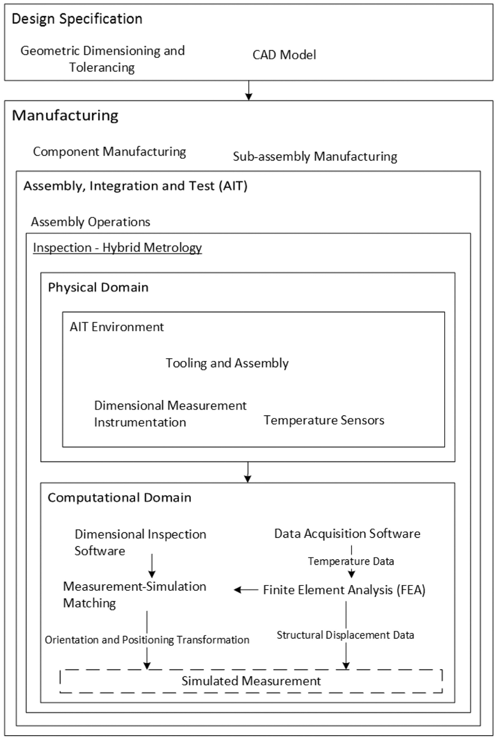
Diagram showing the context of the hybrid metrology approach in the context of manufacturing inspection.
Experimental measurement scenario
Frame structure
The experimental measurand took the form of a cuboidal frame structure. Each of the 12 beam members was made from aluminium 6063 extruded profile by MiniTec and was fastened with proprietary Power-Lock Fasteners. The frame was 2 m in length, and 1 m in height and depth. These dimensions and material choice allowed for experiments to be carried out at the lab-scale while providing maximum thermal expansion.
Supporting this frame were four ball transfer units, which sat at the four bottom corners of the frame. Each of the ball transfer units rested upon flat plates adhered to the floor, which allowed the frame to expand more smoothly. One ball transfer unit was nested in a hole drilled into one of the plates in order to provide a translational constraint. To reset the frame position repeatably and to provide constraint for yaw rotation of the frame, a fiducial post was fixed to the floor for the frame to rest against.
Heating method
At normal ambient temperature, the laboratory environment was relatively stable, varying less than a degree at various positions on the frame. Heating of the structure was performed using a fan heater. Convective heating is the primary heat source in industrial environments, and the fan heater allowed for exaggerated heating in order to significantly observe thermal expansion beyond the uncertainty of the measurement technique. The heater was placed outside of the frame next to the bottom corner, facing inwards.
Metrology
Dimensional metrology – photogrammetry
An AICON DPA photogrammetry system 21 was used for these measurements. A modified Nikon D3X digital single-lens reflex (DSLR) camera equipped with a 28-mm NIKKOR prime lens is used. Image transfer was achieved quickly using a local WiFi connection to a laptop computer. Proprietary software called AICON 3D Studio is used for these measurements and some analysis of measurement data. The 14-bit ANCO-coded targets were fixed to the surface of the structure.
In total, 200–250 images were captured at a range of elevations and orientations around the structure per measurement. Roughly 10 vantage points were used in standing and crouching positions, with eight ladder positions allowing for improved vertical vantage points. In total, each measurement took 15–20 min to complete.
Temperature measurement
Type T thermocouples and class A platinum resistance temperature detectors (RTDs) were used throughout the experiments to measure surface temperature on the frame. Thermal imaging was also carried out to characterise the temperature distribution of the frame when heated by the fan heater.
Thermal images for H2P1 and H1P2 can be seen in Figure 2 showing the magnitude and highly localised nature of the heating.
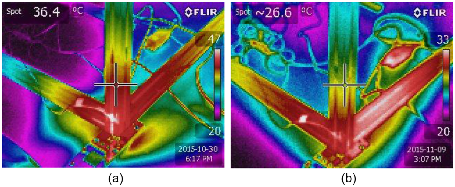
Example thermal images of (a) H2P1 and (b) H1P2.
An FLIR handheld infrared (IR) thermal imaging camera with an absolute accuracy claimed by the manufacturer to be ± 2 °C 22 was used. The sensitivity of the camera is stated as <0.045 °C meaning that the camera is particularly useful in a qualitative capacity for sensor positioning.
Using the thermal images, invasive sensor positions were assigned and can be seen in Figure 3. Sensor density around the heated corner was increased to capture some of the complexity of the localised temperature distribution. Ambient temperature was recorded using a thermocouple (TC0). RTD sensors are more accurate than thermocouples and therefore were used around the heated corner to increase the density in this area. A further 12 thermocouples covered the frame.
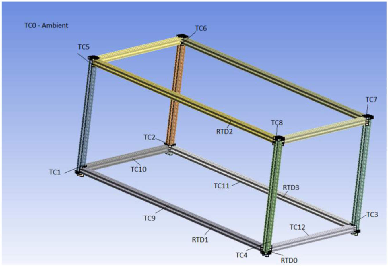
Schematic of sensor positions on frame, where TC1 is the fixed corner and RTD0 is the heated corner.
Computational thermal compensation
Geometry
Simplified CAD geometry was created for the frame to allow for the simulation to run quickly. Chamfers, fillets, and other small details were removed from the geometry. Performing this simplification in the geometry more than halved the simulation run time. Speed of simulation would be important for metrology processes in manufacturing. Figure 3 shows a rendering of the frame, and temperature sensor positions are labelled, where TC0-12 are thermocouples and RTD0-3 are thin-film platinum resistance thermometers.
Simulation – FEA
FEA was used to simulate the thermal expansion under heating. A one-way coupled system was used here in which a thermal analysis is performed to find the full temperature distribution. The results are then passed to the structural analysis, which produces displacement results for each node on the geometry. Relatively coarse meshing is used for both phases of the FEA simulation, again to improve the simulation processing time.
FEA thermal analysis
Over the maximum measurement period, the temperature varied by less than 0.1 °C. As the temperature variation over this period was relatively small, a steady-state thermal analysis was carried out. Average temperature for the period of the dimensional measurement was applied from each sensor at the corresponding FEA coordinates. The initial temperature parameter was set to be the average ambient measurement. Thermal analysis used only a conduction model to calculate temperature at unspecified nodes.
FEA structural analysis
Using the thermal analysis solution, a static structural analysis was performed. Movement of the frame was constrained to match the experiment. The frame is supported using a displacement constraint in the vertical direction, with the horizontal movement unconstrained for three of the points of contact. The ball transfer unit that was constrained in the experiment was similarly constrained in all directions. Displacement solutions along the X, Y, and Z axes were calculated for each node in the simulation.
Target-node matching
Closely matching the coordinate systems of the measurement and the simulation allowed the nearest nodes from the FE mesh to be matched to each photogrammetry target. Measured coordinates were used in a Euclidean nearest neighbour search of the mesh node location data. The corresponding displacement results for the nearest node were used for each photogrammetry target.
Comparison of scaling methods
In addition to simulation, there is also extensive use of temperature measurement in this methodology. Temperature is usually only measured using instrument weather stations unless there is a specific need for enhanced capability, or if the environment is particularly challenging.
Traditional scaling takes a single-scaling factor calculated by multiplying the difference from standard temperature by the CTE, and adding 1 as shown in equation (1)

To separate the benefits of temperature measurement and simulation, the thermal expansion should be calculated for the following:
Traditional scaling – minimal temperature measurement. Mean ambient temperature at the instrument. Mean temperature between maximum and minimum. Worst-case scenario using maximum temperature.
Traditional scaling – full temperature measurement. Mean temperature of all sensors. Median temperature of all sensors.
Hybrid metrology – all sensor data used, and FEA displacements are used to predict expansion.
Results and discussion
Measurement of the structure was performed using the photogrammetry system, and deformation analysis was carried out using the AICON 3D Studio software. The reference measurement H0Px was compared to its heated counterpart HxPx. Both sets of measurement data were initially matched using a best fit of the measured targets to ensure they were both fully aligned. The software then performed a deformation analysis, which calculates the displacement of the targets in the X, Y, and Z directions. Figure 4 shows the regions of interest, with the points measured in each region as well as the heater positions.
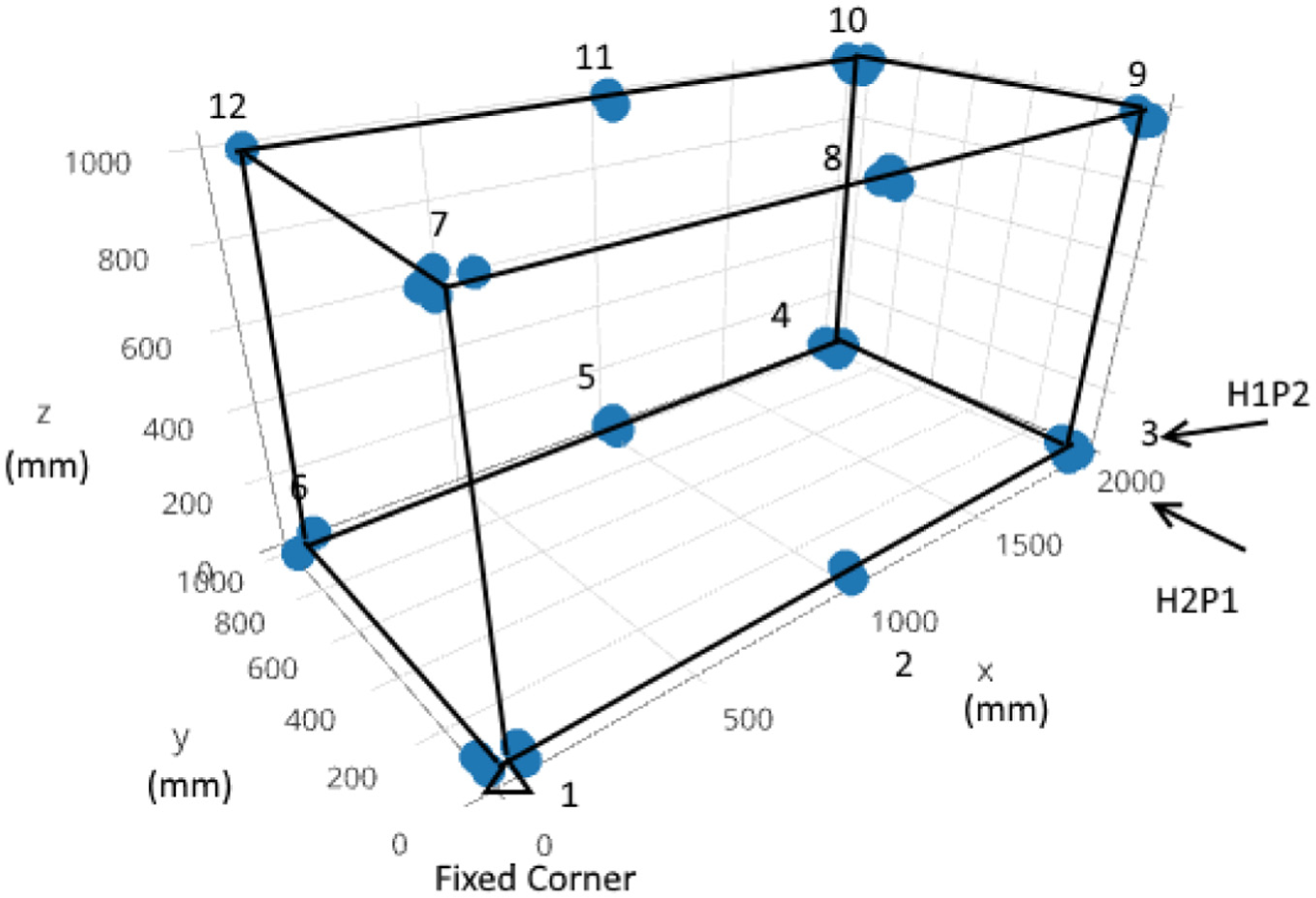
Illustration of the points measured at the numbered regions of interest with fixed point and heater positions.
Scenario 1 – H2P1
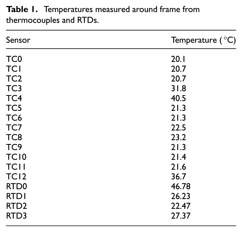
Temperatures in this scenario around the frame are shown in Table 1. Maximum temperature was more than 26 °C above standard temperature.
Temperatures measured around frame from thermocouples and RTDs.
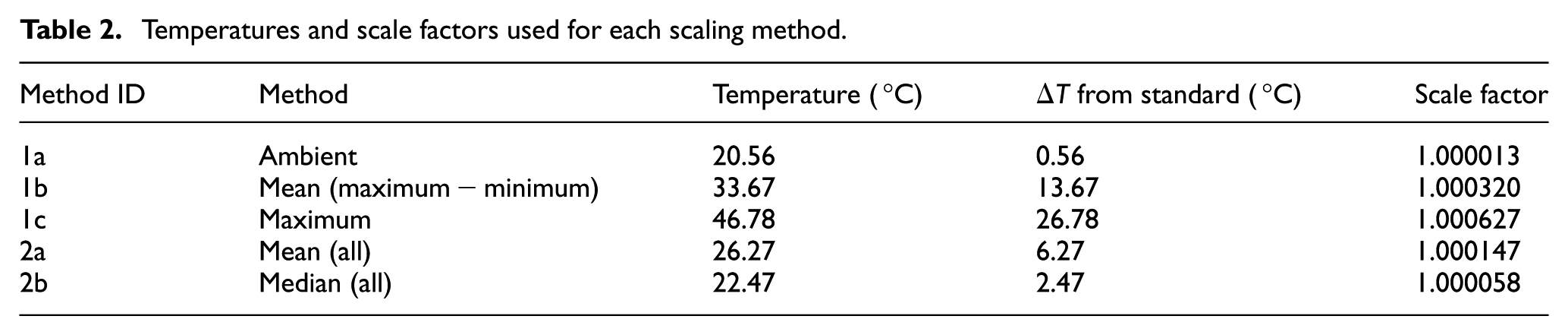
For the traditional scaling techniques, the temperatures used can be seen in Table 2.
Temperatures and scale factors used for each scaling method.
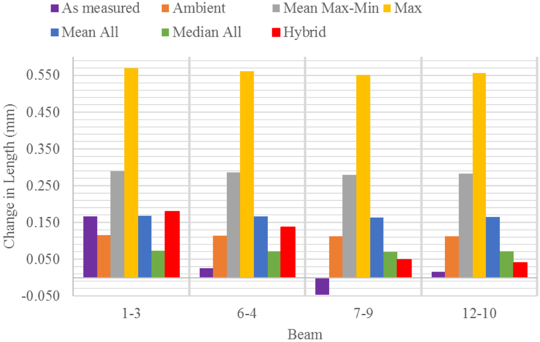
For clarity, the results have been presented for the four 2-m-long beams (Figure 5) and 1-m inter-regional distances for the whole frame (Figure 6). Using methods 1a, 1b, and 1c results in low agreement to the measured results.
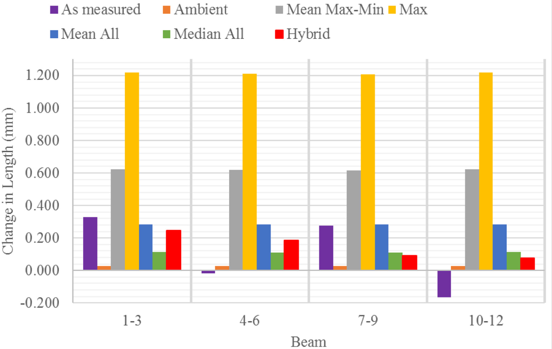
Column chart showing thermal expansion in 2-m beams for all methods compared to the measured value.
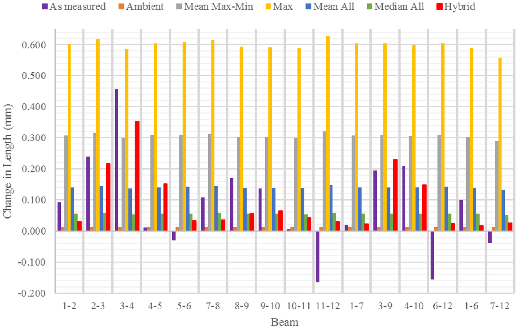
Column chart showing thermal expansion in 1-m beam sections for all methods compared to the measured value.
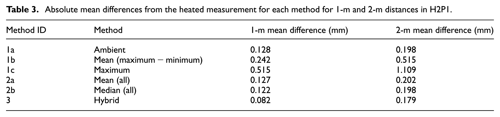
In Figure 6, it can be seen that the ability of method 3 to scale for localised expansion is generally advantageous. Table 3 shows that the hybrid method has a marginally lower mean difference to the measurement results over the various distances compared to other methods.
Absolute mean differences from the heated measurement for each method for 1-m and 2-m distances in H2P1.
Scenario 2 – H1P2
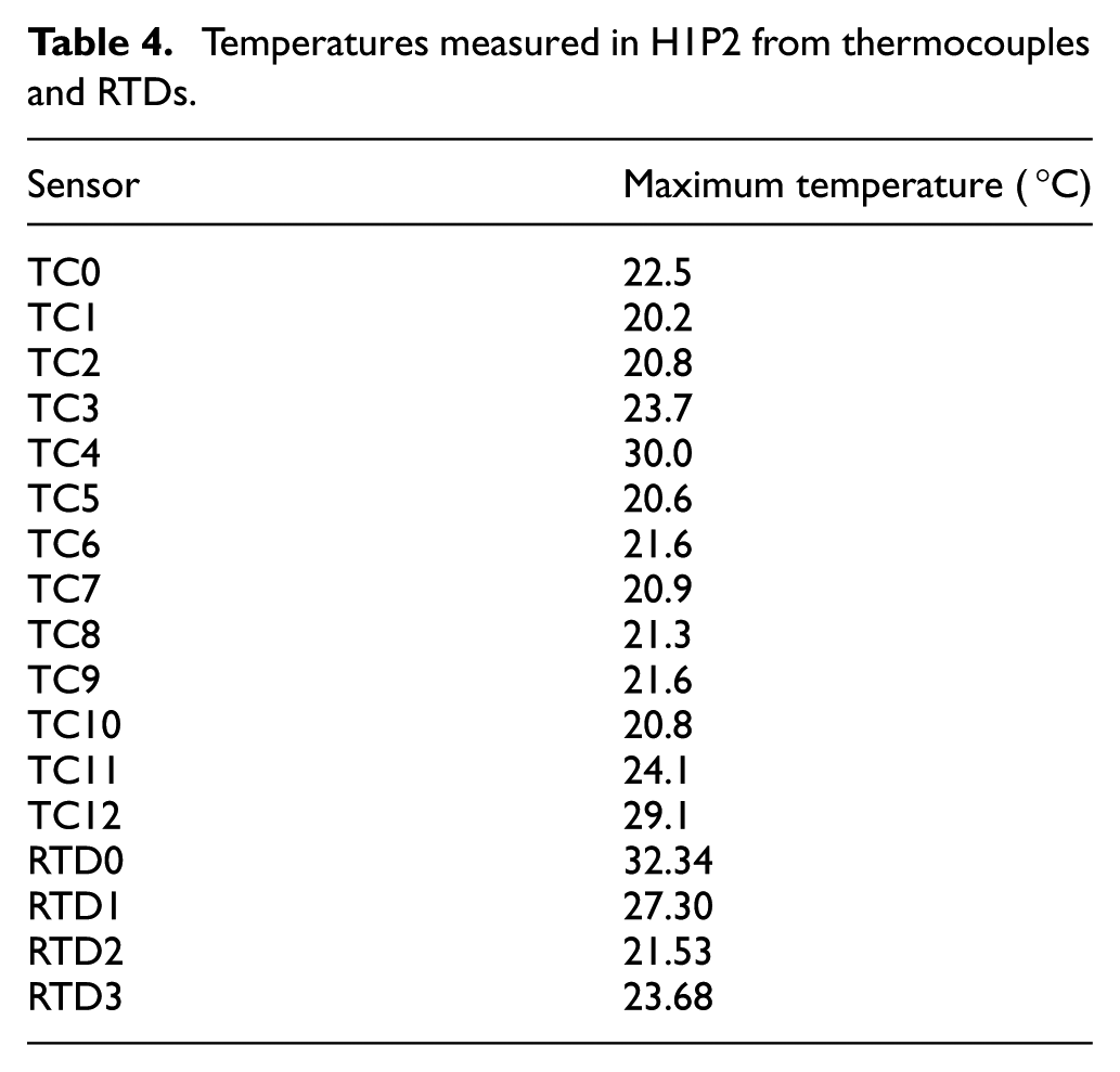
Temperatures in this scenario around the frame are shown in Table 4 and are less extreme than the first scenario. Maximum temperature was in excess of 12 °C above standard temperature.
Temperatures measured in H1P2 from thermocouples and RTDs.
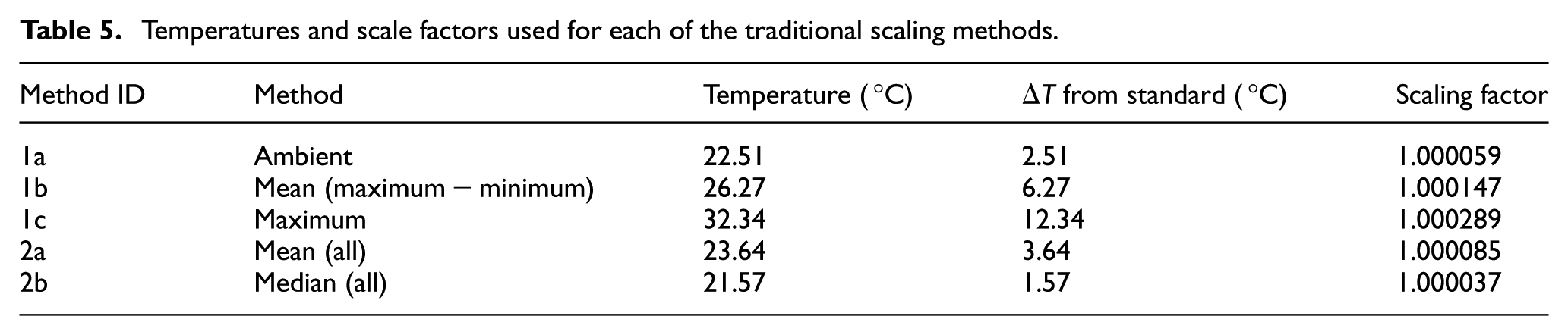
Scaling factors for this scenario can be seen in Table 5. Once again there are a wide range of possible scaling factors due to the localised heating.
Temperatures and scale factors used for each of the traditional scaling methods.
In Figures 7 and 8, we can again see that the hybrid metrology method appears to agree a little more closely with the heated measurements.
Column chart showing thermal expansion of all methods compared to measured value.
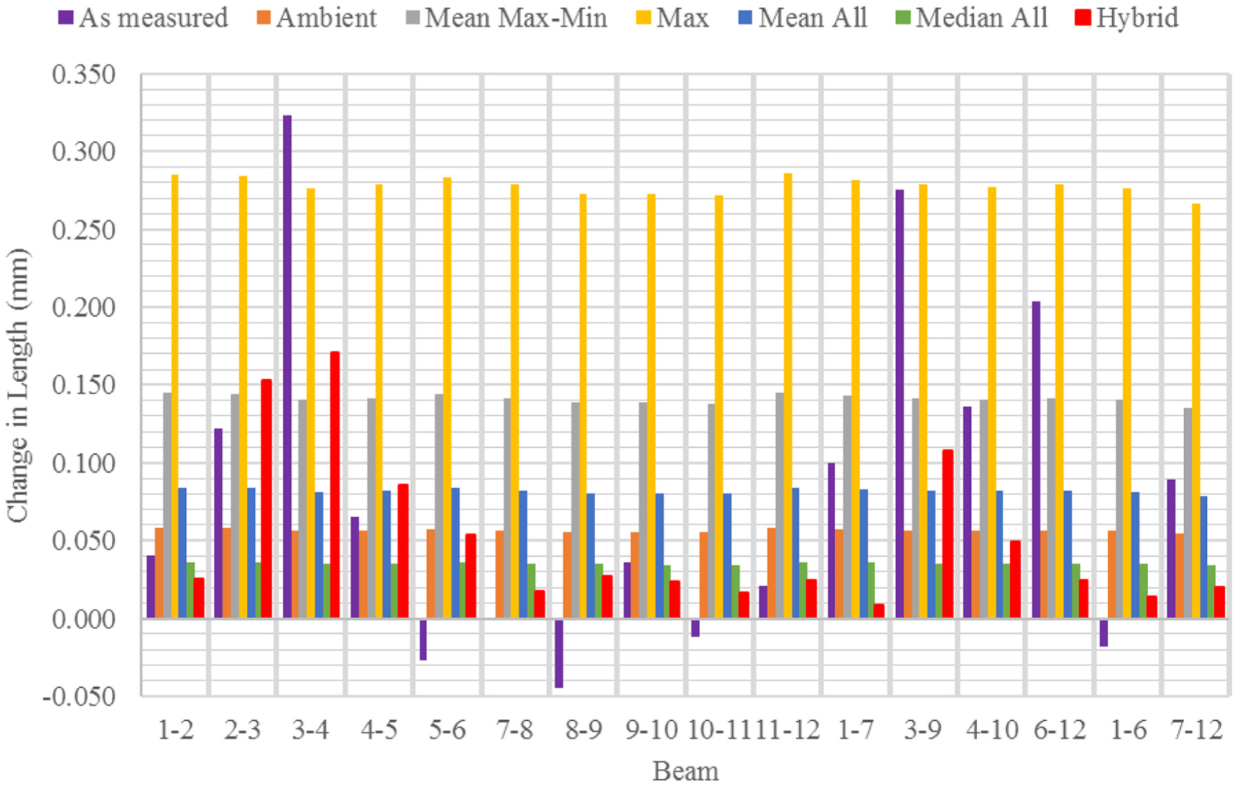
Column chart showing thermal expansion in 1-m beams for all methods compared to the measured value.
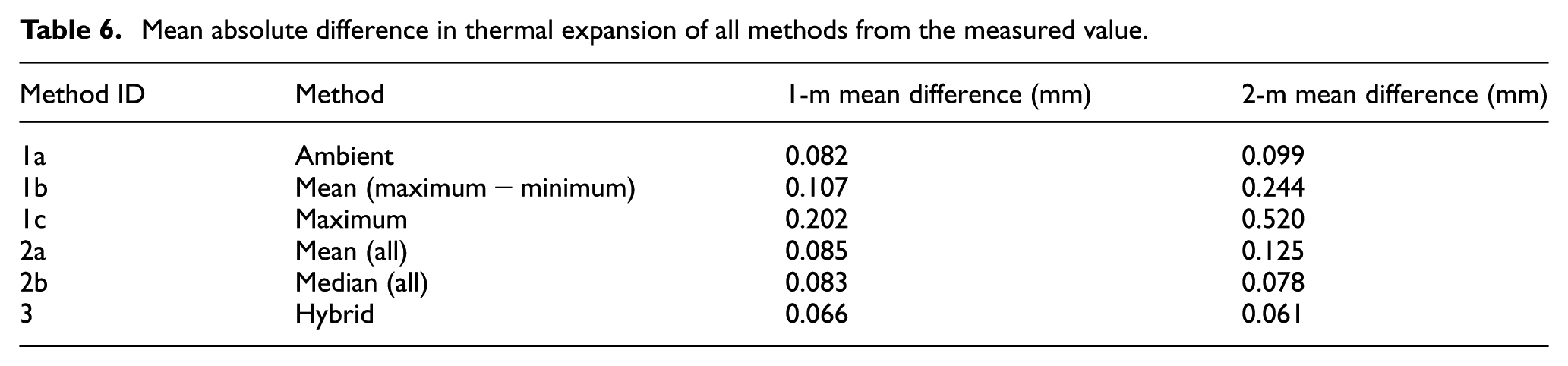
The mean magnitude of difference between the measured results for each of the scaling methods is given in Table 6. Ideal scaling would represent a mean difference tending towards zero, and in this case, it can be seen that the hybrid method generally outperforms than the traditional scaling methods with a mean value of 0.066 mm.
Mean absolute difference in thermal expansion of all methods from the measured value.
The hybrid method can be said to have produced marginally better results than the uniform scaling methods. As the FEA carried out was highly simplified, these results although modest are promising. A number of factors can be improved from this initial study within the simulation to make a far more significant impact to the results. Fine meshing can be used alongside more complex geometry. A transient analysis can be used rather than steady state. The contacts between the beams can also be refined as these are modelled as being more stiff connections than is present in reality. Similarly, the stiffness of the beams themselves can be characterised. Once the finite element model is fully calibrated in this way, the results will become a function of the time spent in setting up the FEA. This is acceptable due to the modular nature of the hybrid metrology approach, where experts in CAD, FEA, and metrology can contribute separately in the initial setup. Ultimately, the major significant finding was the importance of temperature measurement as a far more pronounced difference can be seen from using a full complement of temperature measurement as opposed to one or two sensors.
Conclusion
This article has outlined and shown the application of a straightforward methodology for two things, the first being temperature measurement for dimensional metrology, which is currently often only carried out on the ambient temperature at the instrument. Finite element simulation of displacement allows for compensation of coordinates that would not be possible using current linear scaling methods, due to the presence of highly localised heating.
Two challenging measurement scenarios have experimentally showed that even a highly simplified FEA was able to modestly outperform the traditional scaling methods with both minimal and full temperature measurement.
Thermal compensation is only as effective as the measurement of temperature. Sparsely measured temperature is limited in value and important thermal effects can easily be missed. Temperature measurement is the major contributor to improvement in thermal compensation and can be further improved through the use of simulation.
Future work
Temperature measurement planning needs to be studied further specifically for use in large manufacturing environments so that users can easily optimise their temperature measurement for thermal compensation.
Further experimental studies and consultations with practitioners are to be carried out with a focus on optimising the temperature measurement strategy. Computational studies for temperature measurement planning are under way at the time of writing.
Footnotes
Acknowledgements
The authors thank the industrial collaborators for their contribution, as well as the Department of Mechanical Engineering at the University of Bath.
Declaration of conflicting interest
The author(s) declared no potential conflicts of interest with respect to the research, authorship, and/or publication of this article.
Funding
The author(s) disclosed receipt of the following financial support for the research, authorship, and/or publication of this article: This work was supported by the Engineering and Physical Sciences Research Council (EPSRC) grant EP/K018124/1, ‘The Light Controlled Factory’.