A location prediction method for work-in-process based on frequent trajectory patterns

Abstract

In the data-rich manufacturing environment, the production process of work-in-process is described and presented by trajectories with manufacturing significance. However, advanced approaches for work-in-process trajectory data analytics and prediction are comparatively inadequate. However, the location prediction of moving objects has drawn great attention in the manufacturing field. Yet most approaches for predicting future locations of objects are originally applied in geography domain. When applied to manufacturing shop floor, the prediction results lack manufacturing significance. This article focuses on predicting the next locations of work-in-process in the workshop. First, a data model is introduced to map the geographic trajectories into the logical space, in order to convert the manufacturing information into logical features. Based on the data model, a prediction method is proposed to predict the next locations using frequent trajectory patterns. A series of experiments are performed to examine the prediction method. The experiment results illustrate the impacts of the user-defined factors and prove that the proposed method is effective and efficient.

Introduction

Facing the fiercely competitive environment, manufacturing enterprises need to deal with more and more complicated manufacturing issues in order to improve their production efficiency and to satisfy customer requirements. To achieve this, there is an urgency to apply emerging technologies, for example, smart analytics, advanced prediction tools and cyber-physical systems, to the traditional manufacturing systems.^1,2

As the key factor during the execution process of a manufacturing system, the topic of work-in-process (WIP) control and management aims to monitor WIP inventory and the WIP-level performance for each workstation, material and information flows and to track manufacturing elements, manufacturing resources and production states. WIP control and management occupy an important role in increasing the production efficiency, decreasing the production cost and improving the production quality. For example, investigation of WIP-level performance contributes to bottleneck detection. Hu et al. ³ proposed a dynamic WIP-level control strategy by introducing constraint weights to detect and classify different bottlenecks. Yang and Posner^4,5 established a value-added model by using two heuristic algorithms to minimize the total WIP-level production cost. Li et al. ⁶ indicated that the minimization of WIP inventories might lead to the minimization of production line utilization and proposed a combined objective to improve the flow shop production scheduling. A dynamic system was proposed by Deif and ElMaraghy ⁷ based on mix-leveling policies, aiming to control accumulated WIP level and to manage the capacity scalability, production costs and WIP-level performance. A combined system dynamics approach was used by Filho ⁸ to examine WIP-level utilization in two different manufacturing environments (i.e. single workstation and flow shop) under the influence of six continuous programs (i.e. arrival variability, process variability, defect rate, time to failure, repair time and setup time, as well as lot-size reduction).

The application of Internet of things (IoT) technologies leads to the enhancement of traceability and visibility throughout the production process, contributing to WIP control and management. The supervisory control of radio-frequency identification (RFID)-based systems contributes to accessible and ubiquitous WIP real-time manufacturing data and the tracking of WIP production states.^9,10 Based on RFID application and web service technologies, a real-time WIP management system was proposed to enhance optimal planning, scheduling results and the supervisory during the production process. ¹¹ Fang et al. ¹² proposed an event-driven shop floor WIP management system, in which shop floor events were detected by RFID devices to monitor and control execution dynamics and material handling.

The aggressive application of IoT technologies also establishes the foundation for predictive manufacturing. ¹³ The traditional manufacturing systems focus on visible issues (i.e. the problems and exceptions which have occurred), while invisible issues involve potential and uncertainty. ¹⁴ The production process of WIP is described and analyzed with the huge amount of manufacturing data collected by IoT technologies. With smart analytics and prediction tools, WIP manufacturing data have the potential to be used to predict the next production state and to prevent invisible issues from becoming actual problems. The goal of predictive manufacturing systems is to transform traditional manufacturing objects into smart objects, to create manufacturing intelligence using the knowledge extracted from real-time manufacturing data and to support timely decision making that can deal with invisible issues.^15,16

Despite important progress achieved in the field of WIP management and predictive manufacturing, questions and challenges still exist in using manufacturing data to predict and explain uncertainties. They are summarized as follows:

1. How to use WIP manufacturing data to investigate the production process, to predict the next production state and the potential exceptions? In a traditional manufacturing system, the exceptions do not raise the alarm when they are invisible worries and uncertainties. However, potential exceptions can be discovered by predicting the next locations and states of WIP.

2. How to use WIP manufacturing data to define key issues during the production process and to convert expert experience into logical knowledge? From data mining point of view, the manufacturing data can be used for exception diagnosis, material handling machine process model and logistics control and so on.^17–20 Specific to WIP manufacturing data, WIP trajectories are able to describe key issues only when the manufacturing information is well organized and the extracted knowledge is of manufacturing significance. The logical knowledge extracted from the WIP trajectory data further provides an accurate and reliable description of the manufacturing system, which can be used to explain and express the expert experience.

3. How to improve the planning and scheduling work, how to decrease the difficulty and increase the efficiency at the same time? In traditional manufacturing systems, WIP-level control strategy is generated based on various physical constraints and cost weights, aiming to optimize a single or combined objective. As the complexity of the manufacturing systems increases, the work becomes increasingly difficult and complicated. However, with the predictive analytics, real-time scheduling and decisions can be generated based on the integration of various kinds of knowledge to eliminate the adverse impacts in manufacturing process.

To address the above challenges and questions, this article presents an approach to predict the next locations of WIP based on their trajectory data, which is expected to do some work for predictive manufacturing. There are considerable researches on predicting the next locations of moving objects, but the application specific to WIP is comparatively inadequate. In this article, the approach focuses on the manufacturing significance of WIP trajectories.

The rest of this article is organized as follows. Section “Literature review” provides a brief review on related literature. Section “The logical trajectories” describes a spatial–temporal data model and gives essential definitions. In section “Predicting the next locations,” the approach for predicting the next location of WIP is proposed based on the data model and the frequent trajectory patterns. Section “Experiments” focuses on experiments. Finally, section “Conclusions and further work” presents conclusions and further work.

Literature review

In total, two categories of the literatures are relevant to this article. They are frequent trajectory patterns and predicting next locations.

Frequent trajectory patterns

In the past few years, data miming and advanced analytics have been utilized to investigate the manufacturing system. ²¹ For example, association rule mining was used to identify mapping relationships between important factors in the manufacturing process.^22–24 Meanwhile, another topic is rapidly developing, which is mining trajectory patterns, aiming to discover groups of trajectories based on their spatial or temporal similarity. ²⁵ The movement rules of moving objects are presented by trajectory knowledge and provide a brief and general description of the trajectory database. To extract frequent trajectory patterns, novel algorithms and approaches have been proposed for investigating the moving patterns of objects on road networks, for example, people activities and vehicle trajectories.

For example, Lee et al. ²⁶ proposed a method called graph-based mining (GBM) algorithm to mine frequent trajectory patterns, by employing the depth-first search and adjacent principal. Shaw and Gopalan ²⁷ proposed a method by integrating clustering and sequential pattern mining to extract frequent trajectory patterns. They first divided the trajectory spans area into different clusters, second employed k-means algorithm to refine every cluster and finally applied the sequential pattern mining. Contrary to rigid clusters, Wang et al. ²⁸ proposed an approach with a flexible space partition to avoid sharp bounder problems. Gidófalvi and Pedersen ²⁹ focused on long frequent trajectory patterns which were shared by exponential number of sub-trajectories. They proposed an approach to efficiently extract these long and sharable frequent trajectory patterns by pruning the search space. Not confining to location significance, Abraham and Sojan Lal ³⁰ extracted position and activity knowledge, for example, user behaviors and environment elements, by describing and defining the similarity between spatial–temporal trajectories. Hung et al. ³¹ measured the similarity of the clues of different trajectories to extract movement behaviors for the time durations when no location information is available.

The support of IoT technologies lead to huge amount of ubiquitous and accessible manufacturing data. Researches in this field contribute to logistics control, product life cycle management and manufacturing maintenance.^32,33

A considerable number of researches focus on manufacturing shop floor. As RFID technology has been widely implemented for production and logistics control, the utilization of logistics data is of dominating importance in supply chain research. For example, Kochar and Chhillar ³⁴ proposed a framework based on fuzzy rules to extract the characteristics of the moving objects tagged by RFID devices. Zhong et al. ³⁵ proposed an approach based on RFID-collected logistics data to extract trajectory knowledge. The knowledge was used to visualize the shop floor logistics and to support advanced decision making. ³⁶ Instead of attaching RFID tags to moving objects, Liu et al. ³⁷ used an array of stationary RFID tags to monitor the movements of objects and proposed an application to extract the frequent trajectory patterns.

Predicting next locations

Trajectories specify the path of the moving objects, and trajectory mining plays a vital role in predicting the geographic locations, behaviors and other properties of the objects. ³⁸

For example, Morzy^39,40 proved that the pattern knowledge extracted from historic trajectory data can be successfully used for real-time location prediction. This was done by utilizing a pattern matching algorithm to match the past trajectory of the moving object with movement rules. Jeung et al. ⁴¹ proposed a hybrid prediction model to predict future location accurately for both next and distant locations. They estimated the future motion of an object by its trajectory patterns as well as motion functions. Long et al. ⁴² proposed a general algorithm called Effective, Efficient and Easy Trajectory Prediction (E³TP) to predict motion behaviors of moving objects, which was based on hotspot region mining. Li et al. proposed a novel algorithm to predict trajectory locations. They extracted interesting regions and movement rules from trajectory database and then predicted the locations of moving objects. ⁴³

The next-location prediction gets noticed by enterprises, not only for the geographic position of the next location but also for the behavior significance. For example, Ying et al. ⁴⁴ proposed a novel approach to predict both geographic and semantic behaviors of mobile users. To improve the efficiency, they analyzed all the users and clustered them according to their semantic trajectories and then predicted the next location of a user based on the frequent trajectory patterns in the cluster which the user belonged to. To deal with spatial–temporal trajectory database, a holistic model was proposed to predict next locations by integrating three Markov models.^45,46 The three Markov models, respectively, considered three aspects: all the trajectory patterns in database, the individual patterns of every object and the patterns in similar trajectories. The proposed model was proved effective by the experiments.

From the literature, WIP control is the key factor during the execution process of a manufacturing system. In the data-rich manufacturing environment, the frequent trajectory patterns extracted from the historic data provide vital knowledge of the manufacturing system. However, the advanced approach for WIP trajectory data analytics and prediction is comparatively inadequate. However, the location prediction of moving objects has drawn great attention in the manufacturing field. Yet most approaches for predicting future locations of objects are originally applied in the geography domain. When applied to manufacturing shop floor, the prediction results lack manufacturing significance.

Some problems need further research in the manufacturing environment. They are (1) how to use WIP manufacturing data to investigate the production process and to predict the next production state and the potential exception, (2) how to define key issues of the production process and how to convert expert experience into logical knowledge and (3) how to improve the planning and scheduling work and how to decrease the difficulty and increase the efficiency. To provide core support for dealing with the problems, this article focuses on the next-location prediction of WIP in modern manufacturing environment.

The logical trajectories

In the manufacturing environment, every trajectory in the database specifies a state-changing process of WIP, which contains not merely the geographic coordinates but also the information of the workstations, the processes, information of the workers and the corresponding production time. In this section, a data model is introduced to manage the different types of data, and necessary definitions are claimed based on the model.

The data model

In the manufacturing process, WIP is labeled by a unique attribute Object ID to mark its trajectory. When a WIP reaches a workstation, it is detected by its Object ID, and the corresponding manufacturing information is recorded, for example, the reaching time, the current workstation, the current worker and the production process. Similarly, when WIP leaves a workstation, the information is recorded as well. In this way, the trajectory of WIP specifies its state-changing process.

As shown in Figure 1, the initial state of WIP is represented by S₀ in a multidimensional data cube, which is changing along with the production process. In Figure 1, the data cube details state S_k containing several attributes. The core attribute is Object ID, which is used to define a trajectory. In Figure 1, the values of the attribute Object ID of all the states are the same. Other information is presented in three dimensions. Location dimension indicates the attributes Coordinates and Workstation ID. The value of the attribute Coordinates specifies the geographic coordinates of the current workstation, while the attribute Workstation ID is a unique code for every workstation. Time dimension indicates the attributes Time_b, Time_i and Time_o. Time_b represents the time when WIP enters the buffer. The value of attribute Time_i records the time when WIP is going to be operated for the current process, and the value of attribute Time_o represents the leaving time. Manufacture dimension specifies the attributes Task ID, Material, Process, Product and Quality. Every WIP can be specified by several state data cubes, and these state data cubes indicate the trajectory of the WIP.

Figure 1.

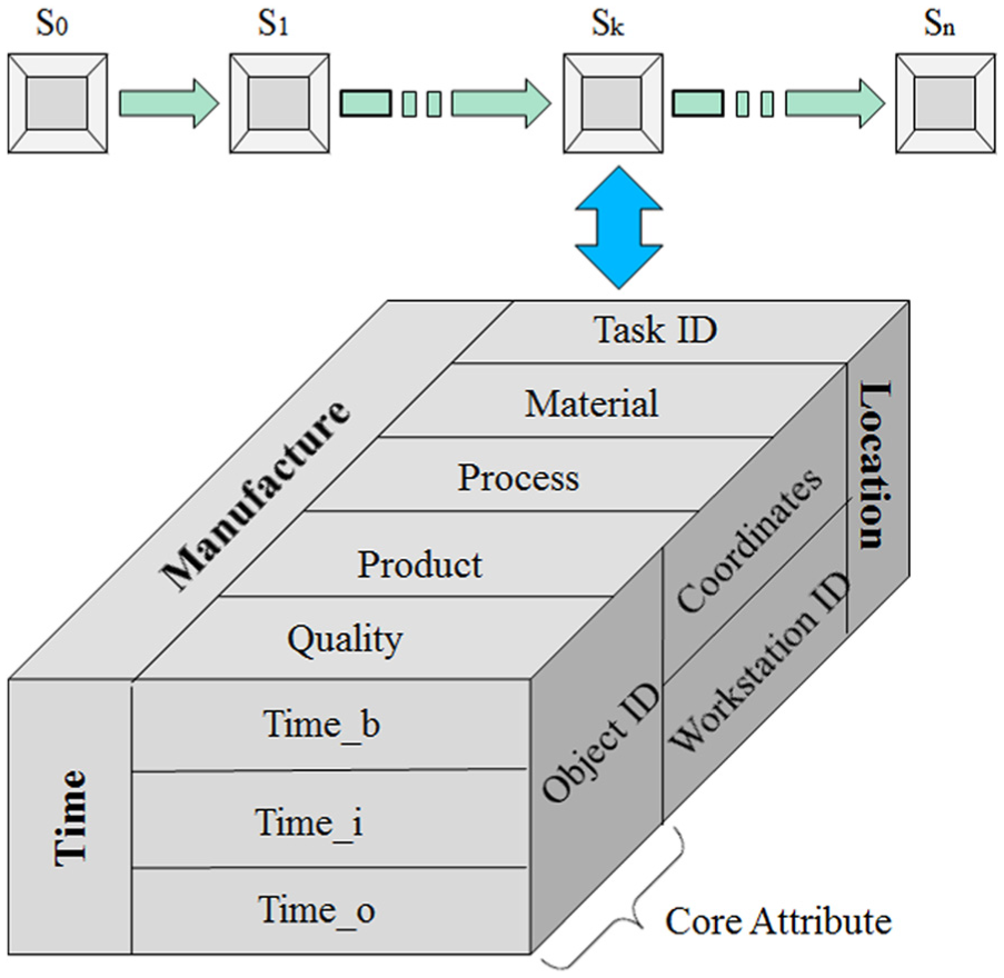
WIP state-changing process with data cubes.

Different from geographic trajectory, the logical trajectory of WIP is presented in the semantic coordinates in Figure 2. Along the process axis, all the possible processes are arranged in the order specified by machining methods and accuracies. Workstation axis labeled the candidate workstations for each process. To achieve this, all the workstations in the workshop are classified into several clusters, and the workstations in the same cluster have the same machining type and accuracy. The workstations in the cluster become candidates for the corresponding process by assigning each cluster to a process. Each workstation in the workshop is labeled by one unique code Workstation ID. The classification work will be more convenient if the unique ID code is determined by the machining types, the accuracies and the serial numbers. Thus, the values along the process axis and workstation axis are discrete. Along the time axis, the values are the results of discretizing the values of coefficient t, representing the relative transport time, which is defined by

$$t_{\mathrm{ji}}=\frac{\mathrm{Time}\_b_{\mathrm{ji}}-\mathrm{Time}\_o_{(j-1)i}}{\mathrm{Time}\_s_{(j-1)i}}$$

(1)

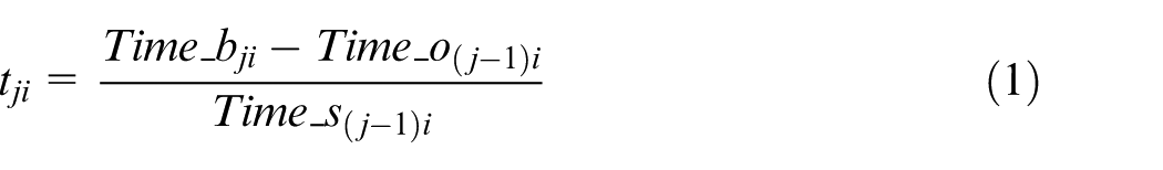
where the subscript i refers to the Object ID of WIP, Time_b_ji denotes the time when WIP(i) enters the buffer, Time_o_(j−1)i indicates the time when WIP(i) leaves the previous operation and Time_s_(j−1)i represents the standard transport time which is a known parameter. Particularly, when the current state is the first (i.e. j = 0), Time_o_(j−1)i denotes the time of exiting the warehouse. Equation (1) evaluates the length of relative transport time linearly on the basis of the standard transport time.

Figure 2.

The logical trajectory of WIP and the process map.

Essential definitions

This subsection displays the necessary definitions. Considering the manufacturing significance contained by the trajectories of WIP, suppose T = {T₁, T₂, T₃, …, T_i, …, T_n}, in which T represents the entire trajectory database and T_i represents the trajectory of WIP(i). The process–workstation plane of the logical space shown in Figure 2 is named “the process map.” In the process map, the values along each axis are labeled by consecutive integers starting from 1. Particularly, the values along time axis are separated into three levels, which represent the short range, the median range and the long range of the relative transport time, respectively. The value of time dimension is marked on each node as the process map is a horizontal plane.

Suppose T_i = (N_1i, N_2i, …, N_ji, …, N_li), in which N_ji represents a node in the trajectory T_i, and node N_ji = (w_ji, p_ji, t_ji). Assume p_ji refers to the current process, w_ji refers to the workstation chosen to perform the process and t_ji refers to the relative transport time defined by equation (1). In the process map of Figure 3, p_ji, w_ji and t_ji are integers. Thus, T_i can be indicated as T_i = [(w_1i, p_1i, t_1i), (w_2i, p_2i, t_2i), …, (w_ji, p_ji, t_ji), …, (w_li, p_li, t_li)].

Figure 3.

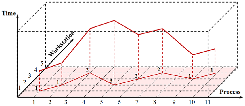
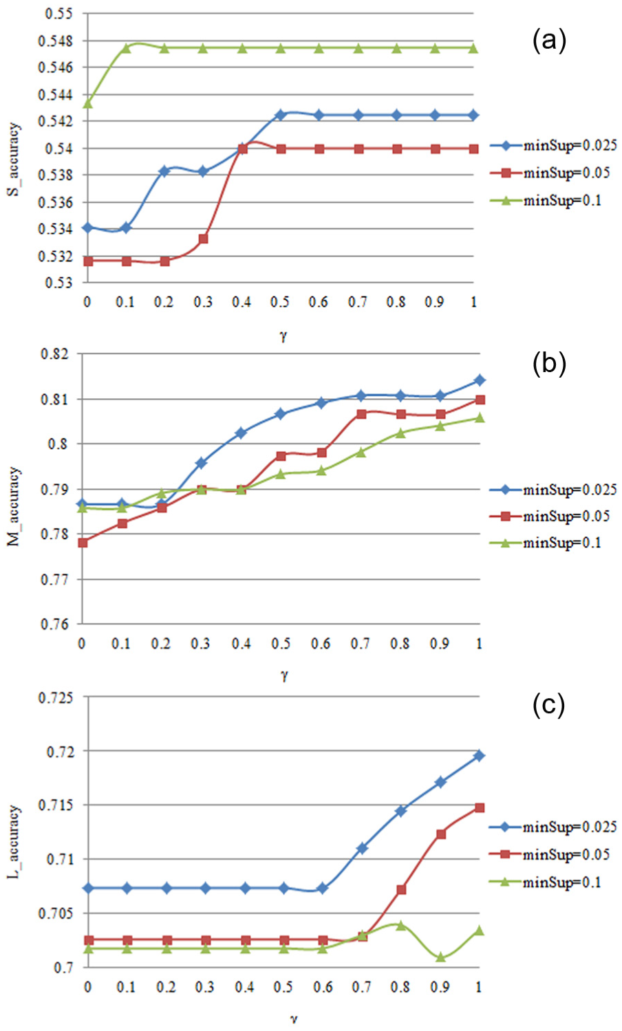
The impact of factor α: (a) S_accuracy versus α, (b) M_accuracy versus α and (c) L_accuracy versus α.

For example, the trajectory in Figure 2 is demonstrated as T_i = [(1, 1, 1), (2, 2, 1), (4, 3, 2), (2, 5, 3), (3, 6, 2), (4, 7, 2), (3, 9, 1), (4, 10, 1)]. The node (4, 3, 2) means that the no. 4 candidate workstation for no. 3 process is chosen to perform the process, and the relative transport time from (2, 2, 1) to (4, 3, 2) is in the median range.

Definition 1

Given a node (w_ji, p_ji, t_ji), the position of the node refers to the position in the process map, which is (w_ji, p_ji) specifically.

It is worth noting that the position of a node means the logical position, and it is not the same as the geographic position of the workstation. The geographic position is specified by the value of the attribute Coordinates of the corresponding state data cube.

Definition 2

Given two nodes (w_ji, p_ji, t_ji) and (w_ki, p_ki, t_ki) in trajectory T_i, if p_ji < p_ki, the process referred by p_ji is performed before the process referred by p_ki, and the node (w_ji, p_ji, t_ji) must be ranged before the node (w_ki, p_ki, t_ki) in T_i.

One trajectory pattern P is defined as P = [(w_k, p_k, t_k), (w_k+1, p_k+1, t_k+1), …, (w_k+m, p_k+m, t_k+m)], in which m is an integer, and the length of the trajectory pattern is valued as m + 1.

Definition 3

The trajectory T_i is defined to contain P (denoted by P ⊆ T_i) if there exists a integer j to ensure that (w_ji, p_ji, t_ji) = (w_k, p_k, t_k), (w_(j+1)i, p_(j+1)i, t_(j+1)i) = (w_k+1, p_k+1, t_k+1), …, (w_(j+m)i, p_(j+m)i, t_(j+m)i) = (w_k+m, p_k+m, t_k+m) and [(w_ji, p_ji, t_ji), (w_(j+1)i, p_(j+1)i, t_(j+1)i), …, (w_(j+m)i, p_(j+m)i, t_(j+m)i)] is a sub-trajectory of T_i.

Definition 4

The support of trajectory pattern P is defined by

$$\mathrm{support}\left(P\right)=\frac{\left|\{T_i|P\subseteq T_i,T_i\in T\}\}\right|}{\left|T\right|}$$

(2)

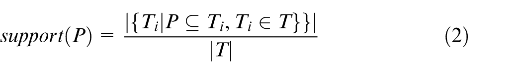
where T refers to the trajectory database and T_i refers to the trajectories in T containing P.

Equation (2) estimates the frequency of pattern P based on the proportion of the trajectories containing P compared to the total number of trajectories.

Definition 5

The minSup is a user-defined factor, which means the minimum support threshold. If the support of a trajectory pattern is not less than minSup, the trajectory pattern is defined as a frequent trajectory pattern.

In this section, a data model is proposed to map the geographic trajectories into logical space, and the essential definitions are declared to explain the features of logical trajectories and frequent trajectory patterns.

Predicting the next locations

In this section, a prediction method is introduced to predict the next locations of WIP. The method is divided into two parts. The first part is preliminary work, which focuses on the frequent trajectory patterns. In addition, other operations required by the prediction method are also included in preliminary work. The second part is prediction work, which plays the major role in predicting the next locations. The two parts are introduced below.

Preliminary work

Frequent trajectory patterns provide a foundation for next-location prediction. However, the patterns are sometimes of a large quantity, especially when the factor minimum support threshold (minSup) is at a pretty low level. Raising the level of minSup is an approach to reduce the amount of frequent trajectory patterns, but a relatively high level of minSup potentially leads to the neglect of some valuable patterns. In order to solve the dilemma, the proposed method is divided into two parts which are preliminary work and prediction work.

It is essential to complete the preliminary work before predicting the next locations, which is mainly about extracting the frequent trajectory patterns. Specifically, all the trajectories in the database are classified into several clusters according to the features of WIP and then the frequent trajectory patterns are generated from every cluster. In manufacturing environment, WIP of the same type generally has similar logical trajectories. In particular, the classification will be quicker and easier if the unique ID code of WIP is determined based on the shape, the material and other physical features. Operating on classificatory trajectory datasets contributes to reducing the computational work and assuring the accuracy of support without neglecting valuable trajectory patterns. However, not all of the WIPs of the same type have similar trajectories. For instance, some WIPs have similar trajectories because of being processed with the same accuracy instead of the same type. In this circumstance, it is more suitable to employ classificatory trajectory datasets and the entire trajectory database at the same time. The preliminary work aims to generate the frequent trajectory patterns with the corresponding values of support and subsequent nodes, from every classificatory trajectory dataset and the entire trajectory database, in which the subsequent nodes are employed to make full use of the frequent trajectory patterns.

In a trajectory database T, suppose P represents a frequent trajectory pattern. Considering the trajectories containing P, the nodes which follow the end of P are candidate subsequent nodes. By adding the candidate N to the last node of P, the formed trajectory pattern is represented by P·N. The confidence of the candidate N is defined by

$$\begin{array}{l}confidence\left(N\right)=\frac{\left|\left\{T_l|P·N\subseteq T_l,T_l\in T\right\}\right|}{\left|\left\{T_i|P\subseteq T_i,T_i\in T\right\}\right|}\\ =\frac{support\left(P·N\right)}{support\left(P\right)}\end{array}$$

(3.1)

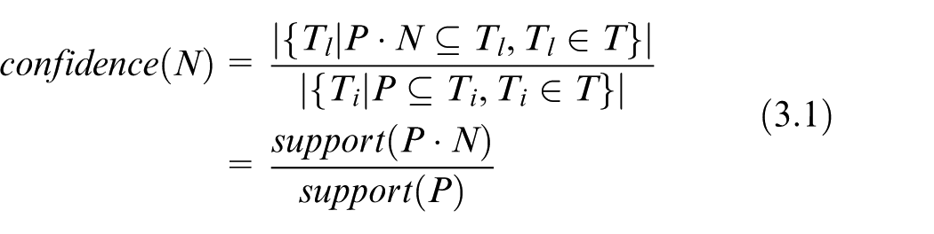
where T_i refers to the trajectories containing P and T_l refers to the trajectories containing P·N.

Exceptionally, the candidate is marked as “end” if there is no node following P. In this circumstance, the confidence is defined by

$$\begin{array}{l}confidence\left(end\right)=\frac{\left|\left\{T_l|P·end\subseteq T_l,T_l\in T\right\}\right|}{\left|\left\{T_i|P\subseteq T_i,T_i\in T\}\right\}\right|}\\ =\frac{support\left(P·end\right)}{support\left(P\right)}\end{array}$$

(3.2)

where T_i refers to the trajectories containing P and T_l refers to the trajectories which end by P.

Equation (3) is used to calculate the conditional probability of every candidate which presents the reliability of the occurrence of the candidate based on the existence of P. For the frequent trajectory pattern P, the subsequent node of P is defined as the candidate with the highest confidence (including the “end” mark). The confidence of the subsequent node is denoted by c_sn.

Definition 6

A Pattern (as presented in Figure 4) is composed of a frequent trajectory pattern, the support and the subsequent node with the corresponding confidence(c_sn).

Figure 4.

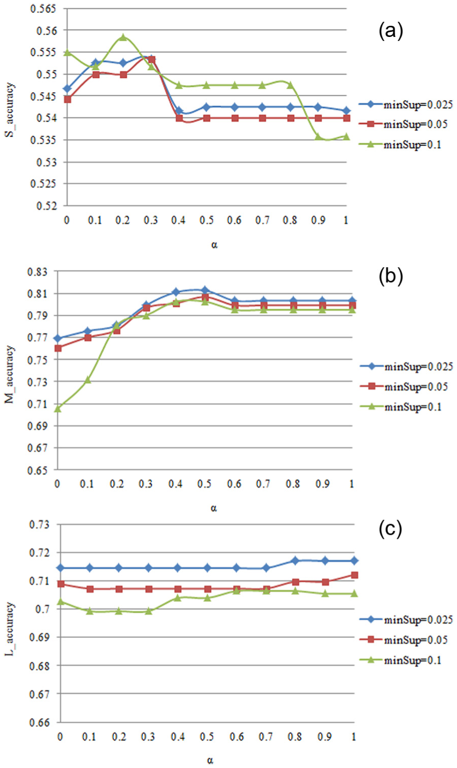
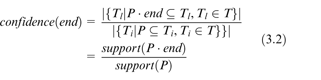
The impact of factor γ: (a) S_accuracy versus γ, (b) M_accuracy versus γ and (c) L_accuracy versus γ.

The preliminary work includes classifying all the trajectories into several clusters according to the features of WIP, extracting Patterns from the entire trajectory database and the classificatory trajectory datasets (equations (3.1) and (3.2)).

Prediction work

The part of prediction work plays a major role in this prediction method. The Patterns extracted from the entire trajectory database and the classificatory trajectory dataset (which the WIP belongs to) are incorporated in next-location prediction. Given the trajectory of WIP’s recent processes, the highest Scores of Matching Results are calculated from both the entire trajectory database and the classificatory trajectory dataset.

Definition 7

Suppose the next location of T_i is to be predicted, and the trajectory pattern P, P ⊆ T_i. A Pattern composed by P is defined as a Matching Pattern of T_i, when there exists two integers r and s, 0 ≤ r ≤ m and 0 ≤ s ≤ r, to ensure that (w_li, p_li) = (w_k+r, p_k+r), (w_(l−1)i, p_(l−1)i) = (w_k+r−1, p_k+r−1), …, (w_(l−s)i, p_(l−s)i) = (w_k+r−s, p_k+r−s), where the positions (w_k+r, p_k+r), (w_k+r−1, p_k+r−1), …, (w_k+r−s, p_k+r−s) belong to a series of consecutive nodes in P, and the value of matching length equals to s + 1.

Considering the trajectory T_i and the Matching Pattern in definition 7, a coefficient δ is defined to describe the matching scenarios of the time stamps. For each pair of matching nodes (w_(l−j)i, p_(l−j)i, t_(l−j)i) and (w_k+r-j, p_k+r-j, t_k+r−j), 0 ≤ j ≤ s, the value of δ(j) is defined by

$$\delta \left(j\right)=\{\begin{array}{c}1,\mathrm{if}{t}_{(l-j)i}=t_{k+r-j}\hfill \\ \multicolumn{1}{c}{d,\mathrm{if}{t}_{(l-j)i}\ne t_{k+r-j}}\end{array}$$

(4)

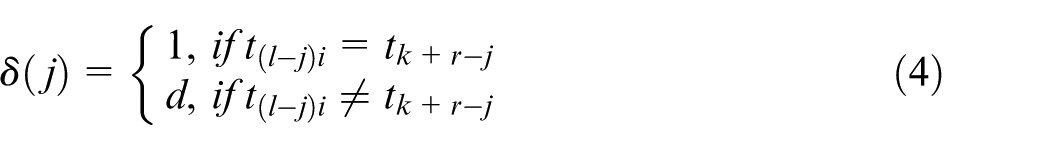
where d is a user-defined factor and 0 < d < 1. Equation (4) indicates that two kinds of matching scenarios of the time stamps go with two values of coefficient δ.

Based on this, the Matching Coefficient is defined by

$$\mathrm{Matching}\_\mathrm{Coefficient}(P,T_i)=\mathrm{support}\left(P\right)*\sum _{j=0}^s\delta \left(j\right)*{\gamma }^j$$

(5)

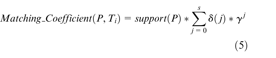
where δ is a coefficient defined by equation (4), and γ is a user-defined factor, 0 < γ ≤ 1. For every pair of matching nodes, the coefficient δ indicates the matching scenarios of the time stamp and coefficient γ indicates the decaying influence. Larger value of γ indicates slower decaying rate.

For the Matching Pattern, the Matching Result is defined to be the node (w_k+r+1, p_k+r+1, t_k+r+1) if the node exists, that is, r + 1 ≤ m, otherwise, the Matching Result is the subsequent node. The Score of the Matching Result is determined by

$$\mathrm{Score}(P,T_i)=C\times \mathrm{Matching}\_\mathrm{Coefficient}(P,T_i)$$

(6)

where $C=\{\begin{array}{c}1,\mathrm{if}r+1\le m\hfill \\ \multicolumn{1}{c}{c_{\mathrm{sn}},\mathrm{else}}\end{array}$

Equation (6) indicates the different scenarios of the Matching Result. The coefficient C indicates the reliability of the result. The value is c_sn when the result is the subsequent node. The value is 1 when the result is the node (w_k+r+1, p_k+r+1, t_k+r+1) because the reliability is 1 according to equation (3) under the circumstance.

In the proposed partial matching strategy, there are four highlighted features: (1) not every node in the trajectory has to match with the frequent trajectory pattern; (2) for each pair of the matching nodes, the positions are defined to be the same, but the time stamps are not; meanwhile, a coefficient δ is defined to describe the possible scenarios; (3) basically, more previous nodes have less potential influence on the predicted result; and (4) generally, higher support of the Matching Pattern and longer matching length make the Matching Coefficient greater.

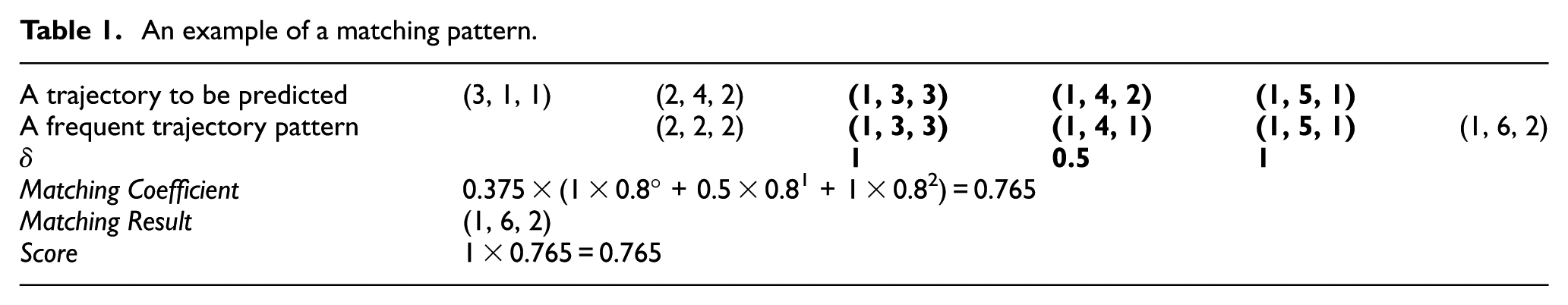
Table 1 provides an example of a Matching Pattern. The support of the frequent trajectory pattern P = [(2, 2, 2) (1, 3, 3) (1, 4, 1) (1, 5, 1) (1, 6, 2)] is 0.375. The factor d is assumed to be 0.5, and the value of γ is set to 0.8. For the trajectory to be predicted, each pair of the matching nodes and the corresponding values of δ are shown in bold.

Table 1.

An example of a matching pattern.

A trajectory to be predicted	(3, 1, 1)	(2, 4, 2)	(1, 3, 3)	(1, 4, 2)	(1, 5, 1)
A frequent trajectory pattern		(2, 2, 2)	(1, 3, 3)	(1, 4, 1)	(1, 5, 1)	(1, 6, 2)
δ			1	0.5	1
Matching Coefficient	0.375 × (1 × 0.8° + 0.5 × 0.81 + 1 × 0.82) = 0.765
Matching Result	(1, 6, 2)
Score	1 × 0.765 = 0.765

The matching list of the classificatory trajectory patterns and the list of all trajectory patterns both contain Matching Patterns and their corresponding Matching Coefficients. From the two matching lists, the result lists generates and records a certain number of Matching Results with the highest values of Score. The two lists are merged into one final result list. For each Matching Result, the value of Final Score is calculated and arranged in order. The Matching Results with the top values of Final Score are Final Prediction Results and are recorded in the final result list.

For each Matching Result in the result lists, the Final Score is defined by

$$\mathrm{Final}\_\mathrm{Score}=\alpha \times \mathrm{Scor}{e}_{\mathrm{class}}+(1-\alpha )\times \mathrm{Scor}{e}_{\mathrm{all}}$$

(7)

where Final_Score denotes the Final Score of the results, Score_class represents the Score calculated from the matching list of the classificatory trajectory patterns and Score_all represents the Score calculated from the matching list of all trajectory patterns. The value of Score_class(Score_all) is set to zero when Score_class(Score_all) does not exist, that is, the corresponding Matching Result does not exist in the matching list of the classificatory trajectory patterns (all trajectory patterns). Moreover, α is a user-defined factor and indicates the influence of classificatory Matching Result on the Final Prediction Result, 0 ≤ α ≤ 1. Equation (7) linearly generates the two kinds of Matching Results. Classificatory Matching Result carries more weight in the Final Prediction Result when the factor α is set to a larger value.

Despite the trajectories of which the next locations can be predicted through the process introduced above, there are some trajectories having no Matching Pattern in the two matching lists. In this circumstance, a special module is employed.

In the special module, the statistic method is applied to determine the prediction results. The trajectories are assumed to be mutually independent in a classificatory trajectory dataset. Suppose the last process in a trajectory is denoted by Ep, the values of Ep of the trajectories in the dataset are mutually independent as well. Therefore, in the classificatory trajectory dataset, the probability of T_i ending with the node (w_li, p_li, t_li) is calculated by

$$\begin{array}{c}\mathrm{Pro}(T_i,\mathrm{end})=\mathrm{Pro}(\mathrm{Ep}=p_{\mathrm{li}}|\mathrm{Ep}\ge p_{\mathrm{li}})=\frac{\mathrm{Pro}(\mathrm{Ep}=p_{\mathrm{li}})}{\mathrm{Pro}(\mathrm{Ep}\ge p_{\mathrm{li}})}\hfill \\ \mathrm{Score}\left(\mathrm{end}\right)=\mathrm{Pro}(T_i,\mathrm{end})\hfill \end{array}$$

(8.1)

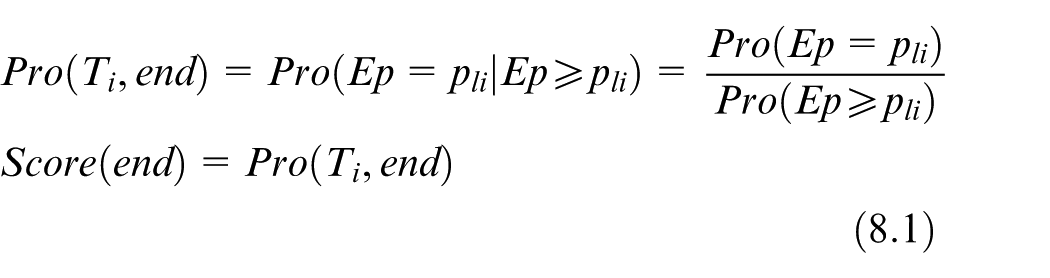
where Score(end) indicates the probability of T_i ending with the current node.

Definition 8

For a node N_c = (w, p, t), N_c is the candidate prediction result if it satisfies two conditions:

1. N_c is a frequent node, that is, a frequent trajectory pattern with the length equal to 1;

2. Assume that p_m represents the defined maximal value on the process axis in the process map, and nk is a user-defined integer (generally 1 ≤ nk ≤ 6). If p_li + n_k ≤ p_m, p_l < p ≤ p_li + nk; otherwise, p_li < p ≤ p_m.

Considering all the candidate prediction results, the Score for each candidate N_c is defined by

$$\mathrm{Score}\left(\mathrm{Nc}\right)=[1-\mathrm{Pro}(T_i,\mathrm{end})]\times \mathrm{support}\left(\mathrm{Nc}\right)$$

(8.2)

Equation (8.2) indicates the reliability of the predicted node N_c by estimating the probability of appearance.

The candidate prediction results (including the probability of ending) are put in the order of Score(N_c) or Score(end) and then the results with the top values of Score are the Final Prediction Results and are recorded in the final result list.

To summarize, the prediction method is decomposed into two parts. Besides the preliminary work introduced in the first subsection, the second part prediction work includes determining the Matching Patterns, Matching Coefficients, Matching Results and the Scores of the trajectory from the classificatory trajectory dataset and the entire trajectory database, respectively; then extracting two result lists (equations (4)–(6)); synthesizing the two result lists into a final result list (equation (7)); and determining the prediction results by employing a special module if no Matching Pattern is found (equations (8.1) and (8.2)).

Experiments

In this section, a series of experiments are presented to examine the performance of the proposed prediction method and to evaluate the influence of the user-defined factors. The experiments were performed on a machine with an Intel(R) Core(TM) i7-3370 CPU 3.40-GHz system with 4.00 GB of RAM. The operation system is Microsoft Windows 7 Ultimate with 64 bit. MATLAB R2012b and Excel are used.

The experiment scenario

The experiments are implemented in a typical discrete manufacturing workshop of a manufacturing enterprise located in Shanghai, China. It is observed that several varieties of products are produced in the workshop. For different varieties of products, the manufacturing processes are greatly different, which leads to the complexity and variability of the execution process. In addition, the features of the manufacturing system are not clear, and the knowledge of the execution process is delivered by expert experiences. When an exception occurs, the reason has to be defined, and the decisions are generated based on expert experiences. For simplicity of description but without losing generality, some essential manufacturing objects and resources are chosen to describe the manufacturing environment.

First, RFID tags are attached to traditional manufacturing objects, for example, WIP, products, materials and automated guided vehicles (AGVs). By this way, they are identified and converted into smart objects. Second, (stationary or portable) RFID readers are deployed on state-changing manufacturing equipment and resources, for example, workstations, buffers, machines and warehouse. In the experiment scenario, each workstation is attached with a waiting area (buffer) for incoming WIP waiting for processing and a finish area for processed WIP waiting for transport. For each workstation, RFID readers are deployed on the entrance of the buffer, the starting point of operation and the exit of the finish area. The tracking of WIP is realized by recording manufacturing and transport information in the identified tags. Third, suitable network devices (i.e. Zigbee and Ethernet) are chosen to transmit manufacturing data. Finally, personal computer (PC) terminal system is constructed to show the manufacturing information, for example, machine conditions, operating records, error reports and configure display of the workshop.

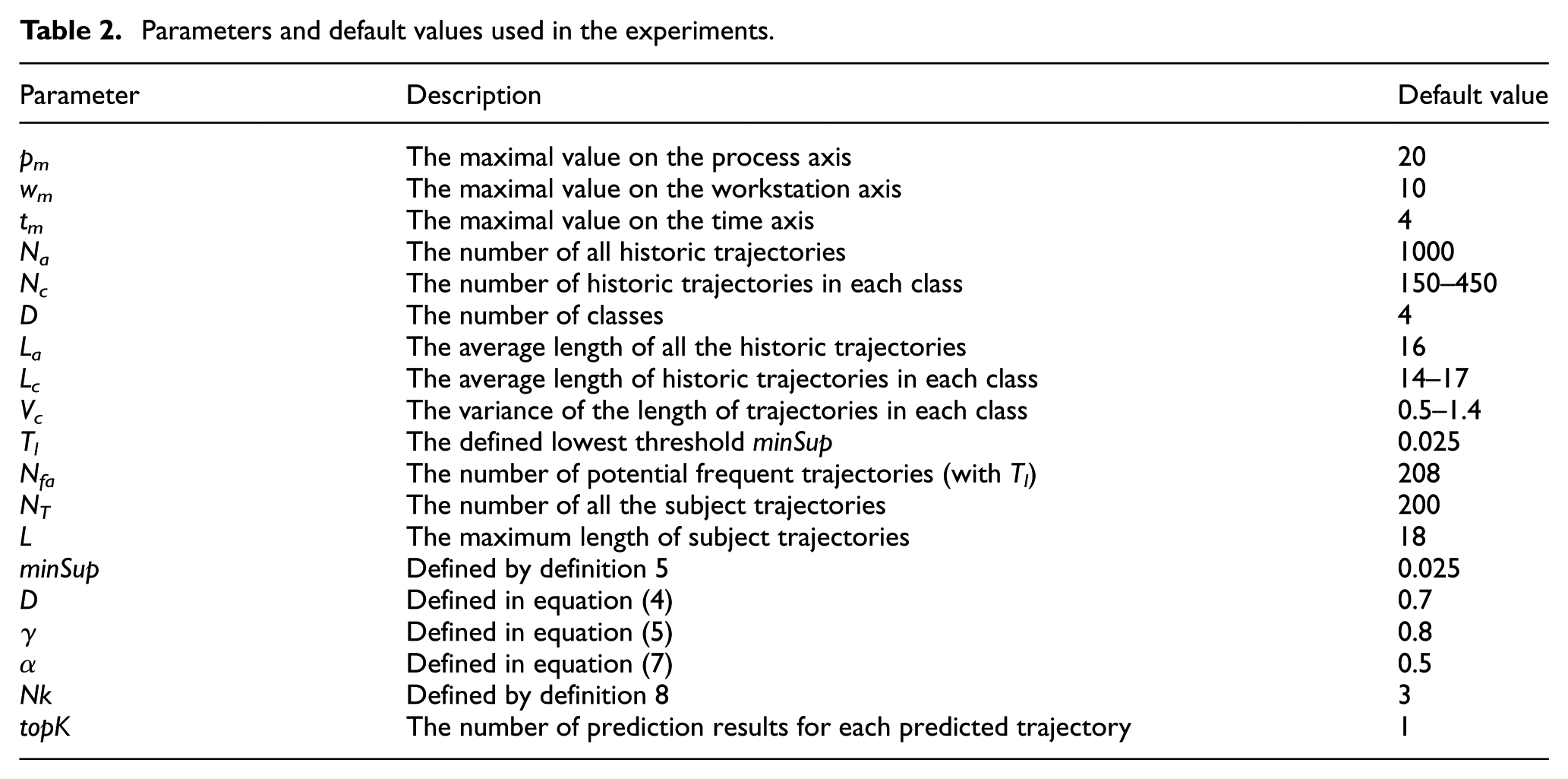
In the experiment scenario, for each transfer task, the transfer distance, the standard velocity and the standard transport time of AGV are known parameters. The WIP production states are divided into three classes: being in waiting, being in processing and being in transit. In total, 20 possible candidate operation processes are lined up based on basic production process. The candidates are selected from the 89 workstations for each operation process. After deleting incorrect and missing data, 1000 WIP trajectories are selected as historic trajectories, and 200 WIP trajectories are chosen to be subject trajectories waiting for prediction. The WIP are divided into four classes based on their geometric features. The range of relative transport time varies from 1.2 to 1.93 and is equally divided into four intervals from 1 to 2. The parameters are shown in Table 2.

Table 2.

Parameters and default values used in the experiments.

Parameter	Description	Default value
pm	The maximal value on the process axis	20
wm	The maximal value on the workstation axis	10
tm	The maximal value on the time axis	4
Na	The number of all historic trajectories	1000
Nc	The number of historic trajectories in each class	150–450
D	The number of classes	4
La	The average length of all the historic trajectories	16
Lc	The average length of historic trajectories in each class	14–17
Vc	The variance of the length of trajectories in each class	0.5–1.4
Tl	The defined lowest threshold minSup	0.025
Nfa	The number of potential frequent trajectories (with Tl)	208
NT	The number of all the subject trajectories	200
L	The maximum length of subject trajectories	18
minSup	Defined by definition 5	0.025
D	Defined in equation (4)	0.7
γ	Defined in equation (5)	0.8
α	Defined in equation (7)	0.5
Nk	Defined by definition 8	3
topK	The number of prediction results for each predicted trajectory	1

Results and evaluations

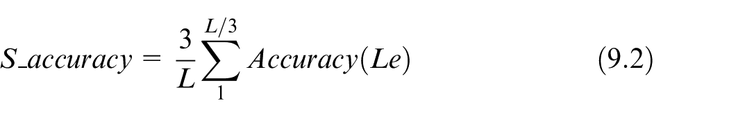
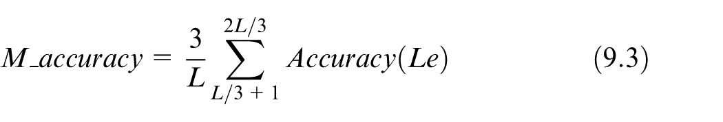
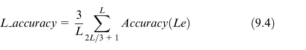
In this subsection, experiment results are presented to illustrate the impacts of the user-defined factors introduced above and to evaluate the performance of the prediction method. To measure the accuracies of the prediction tests, the following measurements are applied, presented by equations (9.1)–(9.5)

$$\mathrm{Accuracy}\left(\mathrm{Le}\right)=\frac{p^{+}\left(\mathrm{Le}\right)}{\mathrm{Ne}}$$

(9.1)

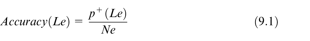
where Le represents the length of the sub-trajectories to be predicted, p⁺ indicates the number of the sub-trajectories predicted correctly and Ne represents the number of the predicted sub-trajectories. Equation (9.1) calculates the proportion of the sub-trajectories which are correctly predicted in the total predicted sub-trajectories

$$S\_\mathrm{accuracy}=\frac{3}{L}\sum _1^{L/3}\mathrm{Accuracy}\left(\mathrm{Le}\right)$$

(9.2)

$$M\_\mathrm{accuracy}=\frac{3}{L}\sum _{L/3+1}^{2L/3}\mathrm{Accuracy}\left(\mathrm{Le}\right)$$

(9.3)

$$L\_\mathrm{accuracy}=\frac{3}{L}\sum _{2L/3+1}^L\mathrm{Accuracy}\left(\mathrm{Le}\right)$$

(9.4)

$$A\_\mathrm{accuracy}=\frac{1}{L}\sum _1^L\mathrm{Accuracy}\left(\mathrm{Le}\right)$$

(9.5)

A set of experiments are implemented for all the subject trajectories, with the user-defined factors set to the default values in Table 2. For each subject trajectory, capture the sub-trajectory by the first Le nodes and predict the next node of the sub-trajectory and then compare the prediction result with the (Le + 1)th node in the subject trajectory. The subject trajectory is excluded from prediction if the length is less than the value of Le. In the experiment, the value of Ne is equal to the value of N_T when 1 ≤ Le ≤ 13, and the shorter subject trajectories are excluded when 14 ≤ Le ≤ 18.

After defining the measurements and indicating the basic features of the prediction accuracies, the tests and evaluations are performed. Experiments indicated below are divided into two parts: (1) illustrating the impacts of user-defined factors and (2) evaluating the performance of the proposed prediction method. In the former part, several groups of experiments are performed under various settings of factors; in the latter part, the efficiency is evaluated compared with previous algorithm.

The impacts of user-defined factors

The influence of factor α is illustrated in Figure 3. This group of experiments is performed with the factors d, γ, nk and topK all set to default values. The factor α indicates the impact of the results from the classificatory trajectory dataset which the WIP belongs to. As shown in Figure 3(a), the prediction accuracy is comparatively higher when the value of α is smaller. This is because the information from the classificatory Matching Patterns is more limited when the sub-trajectories are relatively shorter. Therefore, a larger scope of frequent trajectory patterns is necessary to be taken into consideration. As shown in Figure 3(b), the middle range values of α lead to higher accuracies. It is less reliable to consider only the classificatory trajectory dataset but to make use of the entire trajectory database. As shown in Figure 3(c), larger values of α lead to higher accuracies because the information from their classificatory Matching Patterns is relatively richer, and the results are more reliable when the sub-trajectories are relatively longer.

The influence of factor γ is illustrated in Figure 4. In this group of experiments, the factors d, α, nk and topK are set to default values. The factor γ indicates the decaying influence of the matching nodes. All the test results in Figure 4 illustrate that larger values of factor γ make higher accuracies. This is because lower decay of the influence implies the matching nodes are taken into consideration to a larger degree, and the providing results are more reliable. However, the rising trends of the accuracies are somewhat different. As shown in Figure 4(a), the accuracies stop rising when the value of γ reaches a certain threshold because the information is already limited from shorter sub-trajectories and Matching Patterns. As shown in Figure 4(b), the accuracies continue rising as the value of γ becomes larger when the information is more abundant. In Figure 4(c), the accuracies start rising when the value of γ reaches 0.6, which implies that larger value of γ plays a more important role in rising accuracies because a larger value of γ is necessary to enhance the potential influence for longer sub-trajectories and longer Matching Patterns.

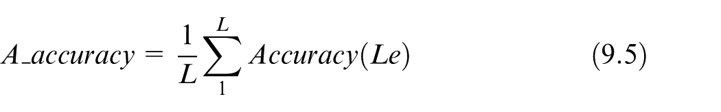
The influence of factor d is illustrated in Figure 5. In this group of experiments, the factors α, γ, nk and topK are set to default values. The factor d indicates the inconsistent matching status of the time stamps. Larger value of d means less reduction of the impact of the matching nodes with inconsistent time stamps. The time stamp represents the relative transport time between two workstations. Higher value of a time stamp indicates longer delay of the transfer task, which implies a more frequent trajectory, a busier transport route or an improper strategy. The influence of factor d is somewhat changeable because inconsistency of time stamps implies different transport conditions. As shown in Figure 5(a), the accuracies go down as the value of d goes up for shorter sub-trajectories because smaller value of d contributes to improving the quality of Matching Patterns when the Matching Patterns are lack of quality and quantity. As shown in Figure 5(b), the accuracies rise slightly as the value of d goes up because larger value of d leads to more Matching Patterns taken into consideration. Moreover, inconsistent time stamps are more reasonable to be tolerated as the sub-trajectories become longer. As shown in Figure 5(c), the accuracies appear basically unaffected by the value of d for the longest sub-trajectories. This is because it is unnecessary to pay much attention to the matching nodes with inconsistent time stamps when the information from Matching Patterns is abundant.

Figure 5.

The impact of factor d: (a) S_accuracy versus d, (b) M_accuracy versus d and (c) L_accuracy versus d.

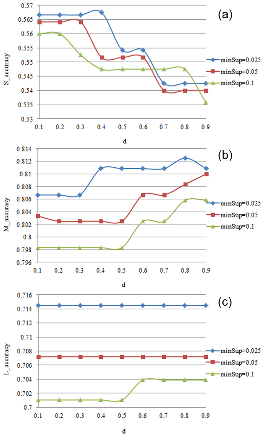
The influence of factor nk is illustrated in Figure 6. In this group of experiments, the factors α, γ, d and topK are set to default values. The factor nk indicates the range where the prediction results are chosen when there is no Matching Pattern found for the sub-trajectory. Larger value of nk means wider size of the range. As shown in Figure 6(a), the accuracies decline as the value of nk becomes larger. This is because it is more likely to find more sub-trajectories with no Matching Pattern, and factor nk appears important for shorter sub-trajectories. Moreover, a smaller value of nk is more appropriate when the value of topK is 1 because it is suitable to choose the result in a narrower and closer range when only one prediction result is picked. When the sub-trajectories are comparatively longer, as shown in Figure 6(b), the accuracies decline much gentler because factor nk is less important when fewer sub-trajectories are found with no Matching Pattern. For the same reason, as shown in Figure 6(c), the accuracies are unaffected by nk at this stage.

Figure 6.

The impact of factor d: (a) S_accuracy versus nk, (b) M_accuracy versus nk and (c) L_accuracy versus nk.

As introduced before, lower value of minSup leads to larger quantity of frequent trajectory patterns. More accurate the values of support, the results extracted from Matching Patterns are more reliable. For these reasons, as shown in Figures 3–6, lower value of minSup makes higher and more reliable accuracy when the sub-trajectories are of mid or long length, but this is not the case when the sub-trajectories are of short length because the role of Matching Patterns is less important in prediction. In addition, the accuracies with the highest minSup are the least robust.

The next group of experiments aims to determine the best setting of factors to maximize the accuracy. The factor topK is mentioned when discussing the influence of factor nk, which indicates the number of the prediction results outputted for each sub-trajectory, as options for future use. As shown in Figure 7, the values of accuracies are rising as the value of topK goes up and gradually converge to a maximum.

Figure 7.

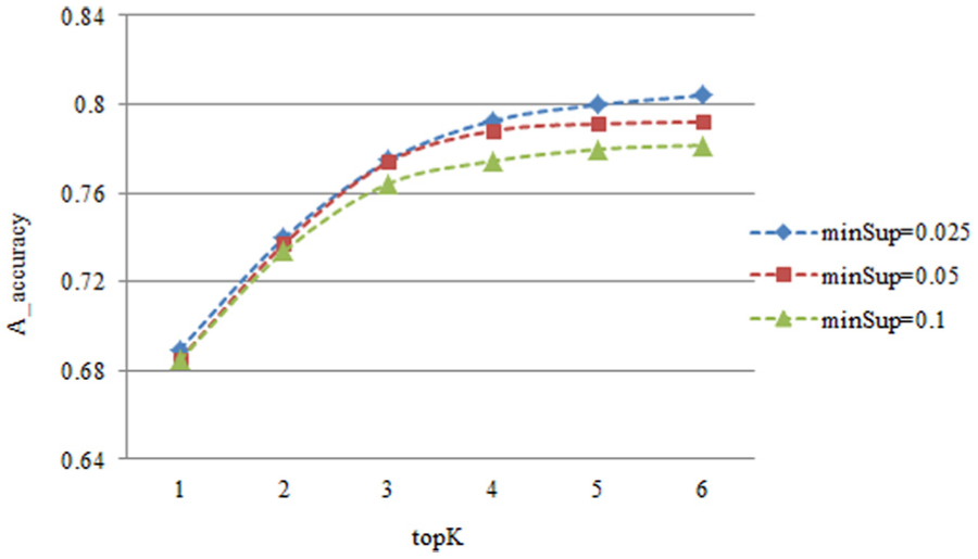
A_accuracy versus topK.

To evaluate the best settings, three setting are determined based on the discussions about the factors minSup, α, γ, d and nk. Setting D refers to default values of factors α, γ, d and nk. Setting A and setting S are concluded from the experiment results shown in Figures 3–6. The values of setting A are determined based on the discussions about how A_accuracy is influenced by factors minSup, α, γ, d and nk. The values of setting S are determined, respectively, based on the discussions about S_accuracy, M_accuracy and L_accuracy.

Figure 8 shows the values of S_accuracy using setting A and setting S with topK set to 6. Despite setting A and setting S are optimized by different ways, the values of S_accuracy calculated based on the two settings are lower than those based on setting D. This is because setting A and setting S are optimized based on the principle that every factors are mutually independent and determined when factor topK is set to 1 (default value).

Figure 8.

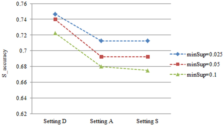
S_accuracy with setting D, setting A and setting S.

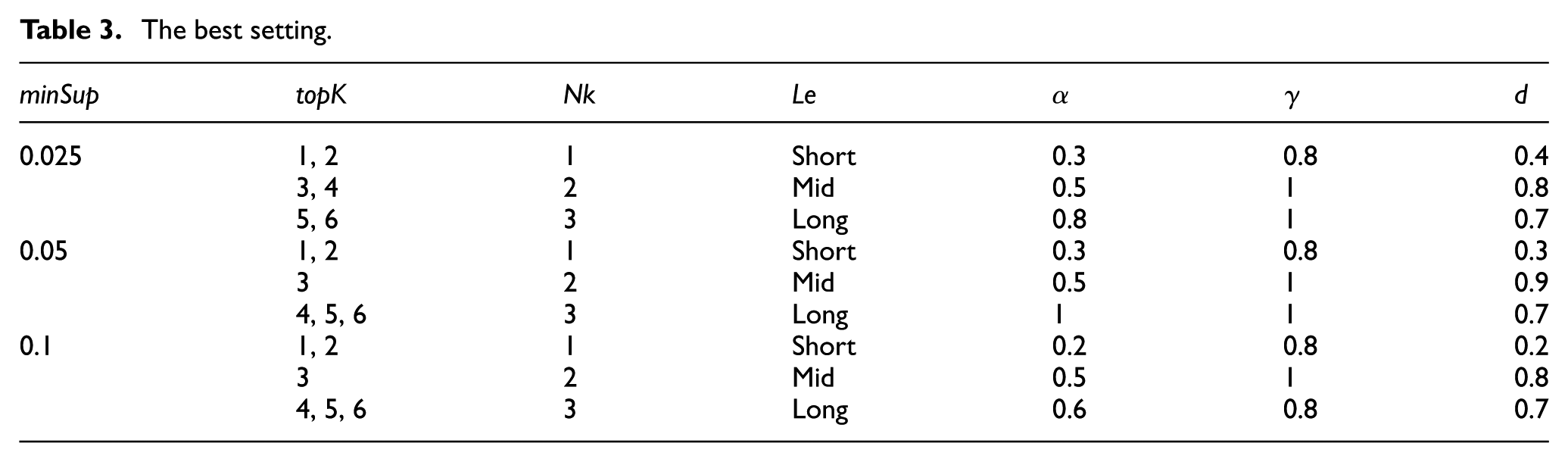
The value of factor topK is not only decided by prediction process but also decided by requirements of other relevant applications. It provides the precondition of other factors. Given a value of topK, the best value of nk is determined, respectively, by an experiment. In this experiment, factors α, γ and d are set according to setting S. Figure 9 shows the results with factor minSup set to 0.025. The best value of nk is marked by number in bold for each value of topK. As shown in Figure 9, when the value of topK is set to 1 and 2, the values of the accuracies are getting smaller as the value of nk becomes larger. This is because a wider range leads to a lower accuracy when the number of picked prediction results is relatively smaller. When the value of topK is larger than 2, the accuracy becomes higher at the beginning, reaches a maximum and then goes lower as the value of nk goes up. The reason for this trend is that a wider range means more options to fit when the number of picked prediction results is relatively greater, but it reduces the probability of picking the correct prediction results when the range is too wide. Determining the best value of nk for each value of topK, the best setting is indicated in Table 3.

Figure 9.

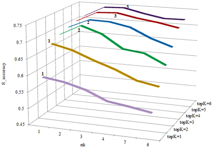
The best value of nk for each topK when minSup = 0.025.

Table 3.

The best setting.

minSup	topK	Nk	Le	α	γ	d
0.025	1, 2	1	Short	0.3	0.8	0.4
	3, 4	2	Mid	0.5	1	0.8
	5, 6	3	Long	0.8	1	0.7
0.05	1, 2	1	Short	0.3	0.8	0.3
	3	2	Mid	0.5	1	0.9
	4, 5, 6	3	Long	1	1	0.7
0.1	1, 2	1	Short	0.2	0.8	0.2
	3	2	Mid	0.5	1	0.8
	4, 5, 6	3	Long	0.6	0.8	0.7

The evaluations of the prediction method

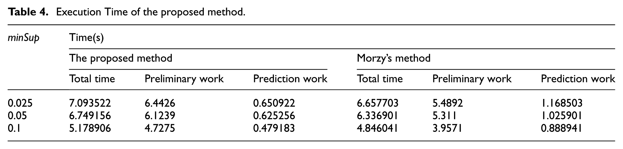
The last group of experiments aims to evaluate the efficiency of the prediction method and to compare it with a previous algorithm proposed by Morzy. ³⁹ Morzy presented a novel method for predicting the location of a moving object by combining it with movement rules. In the experiment, Morzy’s method is modified into the model. The proposed prediction method is implemented on the best setting indicated in Table 3. The results are shown in Table 4 and Figure 10.

Table 4.

Execution Time of the proposed method.

minSup	Time(s)
	The proposed method			Morzy’s method
	Total time	Preliminary work	Prediction work	Total time	Preliminary work	Prediction work
0.025	7.093522	6.4426	0.650922	6.657703	5.4892	1.168503
0.05	6.749156	6.1239	0.625256	6.336901	5.311	1.025901
0.1	5.178906	4.7275	0.479183	4.846041	3.9571	0.888941

Figure 10.

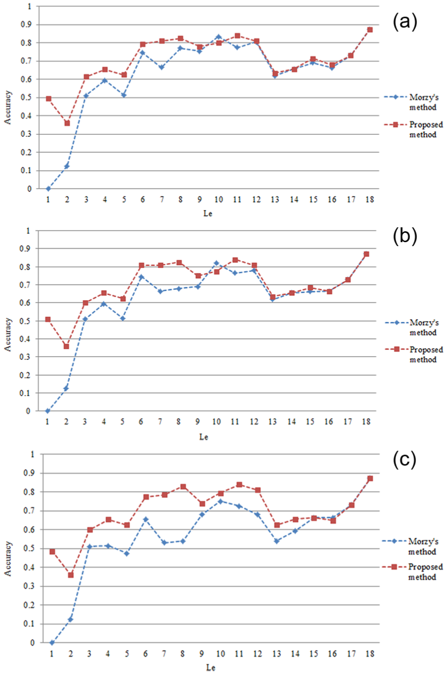
Accuracy comparison between Morzy’s and the proposed method: (a) minSup = 0.025, (b) minSup = 0.05 and (c) minSup = 0.01.

In Table 4, each value of execution time refers to the total completion time of predicting the next locations for Ne sub-trajectories. The preliminary work of Morzy’s previous method contains the calculation of the support and confidence. As shown in Table 4, lower value of minSup leads to longer execution time because there are more frequent trajectory patterns taken into consideration. The prediction method proposed in this article costs more total execution time than Morzy’s previous method does. However, it spends less time on the prediction work. It is appropriate to include the preliminary work into offline module to enhance the real-time efficiency. Figure 10 illustrates the accuracies of the two methods. The accuracy of Morzy’s method is more sensitive to the value of minSup because it only implements on the total trajectory database, while the proposed method utilizes both the total database and the classificatory datasets.

In this subsection, the features of the proposed prediction method are presented by experiments. First, RFID tags and devices are deployed to collect WIP trajectory data. Afterward, the effects of the factors are analyzed, and the best setting is specified to obtain the highest predicting accuracies. Finally, the execution time is indicated and examined.

Discussions

There are several managerial implications in the prediction results. First, the prediction results imply potential busy routes, busy workstations and the deficiencies of current strategy for dealing with invisible issues. It is advised to make adjustments to prevent the potential busy routes from becoming actual transport difficulties, for example, alleviating the current transport strategy, adding branches between the two destinations, widening the current routes, reducing barriers and enhancing the current transport capability.

Second, the prediction rules used in the method provide logical knowledge for accurate description and reliable explanation for investigating the manufacturing system. The logical knowledge is of manufacturing significance, which can be stored, organized, updated and systemized.

Finally, the prediction method contributes to real-time scheduling for reducing the burden and difficulties of the initial planning work. Invisible issues are discovered and defined by predicting the next location and possible state of WIP. For the next stage, real-time strategy for scheduling can be generated by integrating the logical knowledge. Adverse impacts are detected and reduced by eliminating potentials and controlling uncertainties to maintain the execution process.

Conclusion and further work

This article introduces a prediction method to predict the next locations of WIP based on their frequent trajectory patterns, which is expected to do some work for predictive manufacturing. First, a data model is introduced to map the geographic trajectories of WIP into the logical space, aiming to capture and convert the manufacturing information into logical features. The state-changing process of WIP is described and organized by the data model. Second, a prediction method is proposed to predict the next locations for the logical trajectories of WIP based on the data model. The method is divided into two parts, that is, preliminary work focusing on the frequent trajectory patterns and prediction work focusing on the prediction rules. A series of experiments are performed to examine and evaluate the performance of the proposed prediction method. The user-defined factors play their respective roles in the prediction process. The effects of the factors are analyzed, and the execution time is evaluated, to describe the features of the proposed prediction method.

The main contributions of this article involve the following: (1) an abstraction of the workshop production process is proposed based on multidimensional data cubes. By the process map, the geographic trajectory of WIP is mapped into logical space to describe the logical features of the manufacturing system; (2) a prediction method is proposed to predict the next locations and possible states of WIP, based on the logical trajectories presented by the data model. The prediction results are used to detect and defined potentials and uncertainties, which contributes to dealing with invisible issues during the execution process. Several experiments are performed to examine and evaluate the performance of the prediction method; and (3) the prediction rules provide logical knowledge for accurate description and reliable explanation of the manufacturing system. With the prediction results and the logical knowledge, the real-time scheduling strategy can be generated to reduce the difficulties of the initial scheduling work and to eliminate the adverse impacts during the execution process.

Future work will be performed as follows. First, although the data model and the prediction method are proposed, there are several issues to be explored in the future work, which includes two aspects. For the data model, the logical meanings are in need of further research to enhance the spatial–temporal features of the trajectories and to achieve a higher level of abstraction. For the proposed prediction method, the statistics method applied in the prediction method needs improvement. Second, the position–action–service model of workshop is to be established based on the fusion of the physical space and the logical space. Further research involves the comprehensive relation between the production status of every WIP and the real-time location data. Finally, an optimizing mechanism is to be proposed to integrate the real-time manufacturing data with the production process.