
Abstract
For revolving components like compressor stages in aero-engine, it is critical to ensure that the overall concentric performance of the assembly is extremely excellent to satisfy the requirements of vibration-free and noise-free. However, in practical production, it is hard to meet the target requirement by manual adjustments; in virtual assembly, it is difficult to build an effective deviation propagation model with traditional methods. This article focuses on two points: one is the assembly technique of multistage rotational optimization and the other is the deviation propagation model for revolving components assembly. The revolution joint was introduced in the unified Jacobian–Torsor model to provide the rotary regulating effects. This modified model has advantages of being able to consider rotating optimization, geometric tolerance, and percentage contribution compared with other mathematical methods. General formulas for the n-stage components assembly were derived including the deviation propagation function and optimization destination expression. Comparisons between three assembly techniques and experiments were made to prove the suggested method was feasible and of high practicability. It can be integrated with computer-aided design systems to propose assistance for operators in assembling stage or redesign parts tolerances where FEs’ percentage contributions can be obtained in design preliminary stage.
Keywords
Introduction
The high-speed rotating components are widely used in the aero-engine modules. To improve manufacturability and maintainability, a core engine is almost always manufactured as an assembly of individual parts, and assembly deviations are unavoidable because of geometrical errors. As the key part of an aircraft, engine assembly quality casts significant influence on its fatigue durability and aerodynamic characteristics. Revolving axisymmetric components, such as compressor stages which are the core of aero-engine, 1 they need to be assembled by restricting the concentricity deviation to be within a micron-sized tolerance to satisfy the requirements of vibration-free and noise-free. 2 Assembly variation analysis is a practical method to control the deviation propagation. Whether in the assembling stage or in product development stage, appropriately modeling the deviation propagation and optimizing the erection scheme can efficiently improve the product quality and cut down the cost and time of design cycle. 3
However, nowadays very few computer-aided design (CAD) systems propose assistance for operating personnel in the arduous task for aero-engine assembly. Two or three workers spend nearly 4–5 days to complete the installation task, and it is hardly to meet the target requirement by manual adjustments. This article attempts to propose an innovative assembly technique whose mathematical algorithm can be integrated with the CAD systems. With the aid of some tolerance analysis method, 4 geometrical information can be fully considered, and analysis results are conducive to guiding actual assembling and parts tolerances redesign.
Generally, the traditional methods for studying deviation propagation are based on engineering experience or one-/two-dimensional (1D/2D) chain,5–8 which are inadequate for the geometric deviation analysis in three-dimensional (3D) spatial state. 3D tolerance analysis methods have been studied to deal with geometric variations 9 over the past three decades. Orientation, location, and form information ignored by traditional 1D/2D tolerance analysis methods can be considered by 3D methods. It should be noted that deviation analysis is other than tolerance analysis. The former pays attention to the imperfections in manufacturing processes, and the latter places emphasis on tolerance specification of parts. But they have the similar stackup effects of deviations/tolerances from parts to functional requirements (FR) of assemblies. Therefore, the propagation models are appropriate for both of them.
Copious 3D tolerance propagation models have been proposed and developed according to some latest literature review studies.10–12 The kinematic formulation, 13 the network of zones and datums, 14 and the spatial dimensional chain 15 were included in the preliminary explorations. Thereafter, the variational method,16,17 the direct linearization method (DLM), 18 Jacobian matrix transfer model, 19 Torsor model,20–22 Tolerance-Map (T-Map) approach, 23 matrix approach, 24 and unified Jacobian–Torsor (J-T) model 25 have achieved remarkably developed. In recent years, meta-modeling approach, 26 polychromatic sets-based model, 27 and shortest path graph 28 were presented successively. Four major 3D models among them have been widely reported and deeply researched, that is the DLM model, the T-Map model, the matrix model, and the J-T model.
The DLM18,29 uses vectors to express both assembly dimensions and component dimensions. All the types of tolerances can be easily constructed; however, how to model the closing vector-loop and define the joint types mostly relies on the user’s experience and expertise. It will cause inconclusive tolerance synthesis results when people choose diversified vector paths of the vector-loop tolerance model. Moreover, the DLM has not fully considered the tolerancing standard conformance between the dimensional tolerance and the geometric tolerance. A hypothetical Euclidean volume is utilized for the T-Map model23,30 which absolutely coheres with the ASME/ISO standard, but only 1D tolerance analysis has been attempted in a practical application, and the tolerance propagation adopting Minkowski operation is cumbersome and tedious. Meanwhile, the statistical algorithm of T-Map is still at the starting stage, whose application is basically a blank. This causes the solution of sensitivity and percent contribution is unable to achieve. Moreover, a four-dimensional (4D) and even higher-dimensional T-Map is difficult for visualization. A displacement matrix is adopted in the matrix model24,31 to characterize each feature’s small displacements in a limited range of specified tolerances. It can be easily integrated into CAD programs because of its simplicity and easy comprehension; however, the calculation procedure is inherently inefficient as a result of the huge amount of nonlinear inequalities and other constraint conditions. This point-based tolerance analysis model results in uncertain results when people select different points as constraint objective and analysis objective. The J-T model25,32 combines the advantages of the Torsor model which is suitable for tolerance representation and the Jacobian matrix which is suitable for tolerance propagation. Statistical algorithm33–36 has been studied fairly well and this model has been refined over the last decade,37–39 but it is not perfect for partial parallel chain problem.40,41
Combined with the rotor’s configuration and assembling characteristics of aero-engine, the J-T model will be adopted for an in-depth study of multistage rotational optimization, which is very suitable for complex assemblies that contain a large number of joints and geometric tolerances. Although the J-T model could be more accurately used for assembly tolerances redesigning where each functional element’s percentage contribution (PC) can be solved, it cannot be directly applied into optimization-oriented operation. That is, it cannot be used to evaluate and optimize assembly scheme on the basis of existing tolerance proposal. Normally, assembly quality of the product largely depends upon the product type and the optimization technique. For the revolving axisymmetric components, they possess the special properties that each component can be adjusted to the most suitable orientation to meet the best performance of the final assembly. Recently, Yang et al. 42 and Hussain et al. 43 studied the optimization techniques for controlling the variation propagation in the aero-engine assembly. Three procedures were studied for optimizing the assembly of components stack in two dimensions, which are limited in the practical fully 3D case. After that, they developed straight-build 44 and parallelism-build 45 assembly in three dimensions considering various levels of process noise, measurement accuracy, and available orientations, and a probabilistic approach was proposed as well. 46 However, the above-mentioned assembly technique could not fully consider the influence of geometric tolerances, and the optimization objective only focused on the concentricity of the top-stage component, which was not the optimal solution for the overall assembly.
To solve this problem, the concept of revolution joint is introduced in the traditional J-T model, which can provide the rotary regulating effect for each component. An assembly process targeted at satisfying the minimum concentricity deviation for the overall aero-engine is named as “multistage rotational optimization,” corresponding to “top-stage optimization” which is focusing on the concentricity of the top-stage component only. By the modified J-T model, parts geometrical information will be fully considered, and optimal installation angles and PCs can be calculated.
This article focuses on two points: one is to propose a novel assembly technique of multistage rotational optimization, and the other is to build the 3D deviation propagation model for revolving components assembly. The J-T model with the revolution joint will be used to explore the general formulas for n-stage components assembly. Comparisons between different assembly techniques and experiments will be made to show advantages of this suggested method that it can easily express the part-to-part relationships, predict the final assembly quality, and be used to search the optimal installation angles to propose assistance for operating personnel.
Assembly technique of multistage rotational optimization
In the assembling process for the revolving axisymmetric components, concentricity variation could be kept to the minimum by rotating the component around its axis of revolution stage by stage. This article considers the actual operation of assembly to provide effective and economical solutions to analyze variation stackup and control variation propagation.
Description of unified J-T model
The J-T model which is the essential method adopted in this article consists of the Jacobian matrix and the Torsor model. A Torsor model uses three rotational vectors and three translational vectors, respectively, to express the orientation and position for an ideal surface. Supposing S0 is the nominal position and S1 is an arbitrary variational surface relative to S0 with tolerance T, the Torsor model of S1 which represents position and orientation with respect to S0 can be represented as

where u, v, and w are three translation vectors on the x-,y-, and z-axes in local reference system, respectively; likewise, α, β, and γ are the rotating vectors around the x-, y-, and z-axes, respectively.
It is noteworthy that tolerances only have practical significance in direction differ from those which leave an invariant surface in regard to itself. 47 That is, in a Torsor model, the number of effective vectors equals to the non-invariant degrees of a characteristic element. According to the displacements set theory which is proposed by Hervé, 48 some vectors of seven primary Torsor models in equation (1) can be set to zero, as shown in Table 1, to simplify the computational process.
Features and their Torsor models.
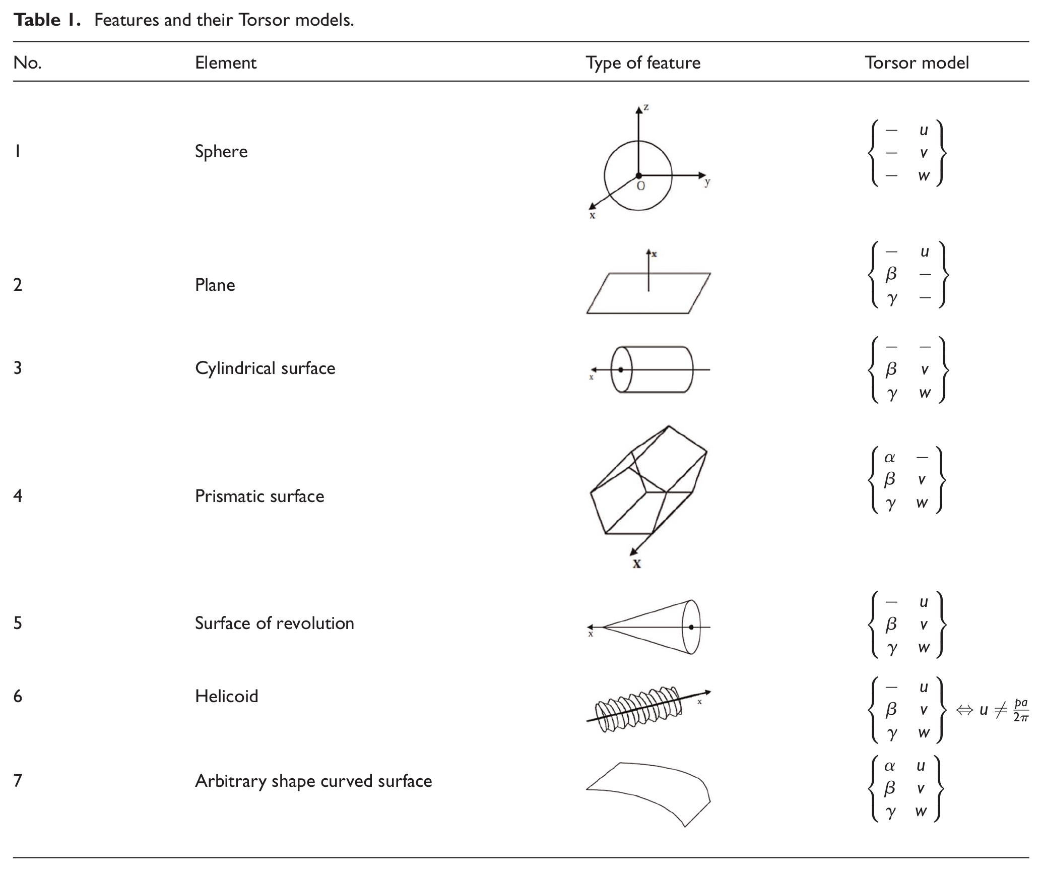
In Table 1, u, v, and w are three translation vectors on the x-, y-, and z-axes in local reference system, respectively; likewise, α, β, and γ are the rotating vectors around the x-, y-, and z-axes, respectively. “–” indicates that the vector has no effect on corresponding tolerance change in that direction. p and a represent screw pitch and thread tooth link angle, respectively.
These vectors are transferred to the objective controlled variable by virtue of the Jacobian matrix. Jacobian matrixes describe relative positions, as well as relative orientations between local reference frames and the global reference frame. The unified J-T model has the synthesized advantages with Jacobian matrix that is good at tolerance propagation and Torsor model that is appropriate for tolerance representation.49,50 The complete J-T model can be formulated as equation (2)
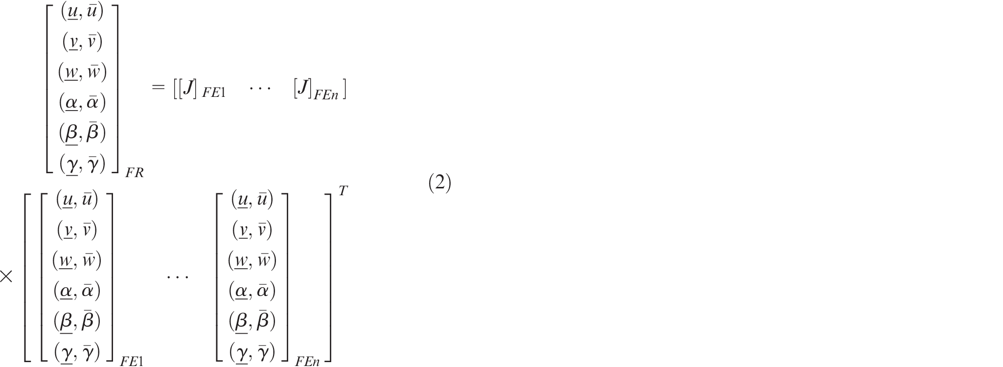
where α, β, γ, u, v, and w are the same with those in equation (1); n indicates the number of the functional elements (FEs);
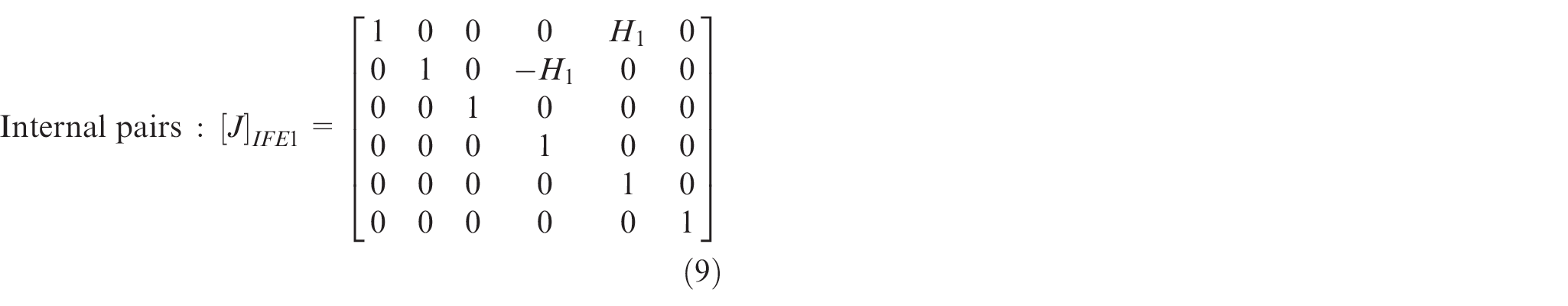
There are two categories for FE pairs in one assembly, that is the internal FE (IFE) pairs which consist of two FEs on the identical parts, and contact FE (CFE) pairs which are composed of two FEs on the diverse parts if there exists potential or physical contact between them. Each FE pair’s variations will be transferred to the FR with Jacobian matrix, by which the ith FE can be expressed as follows
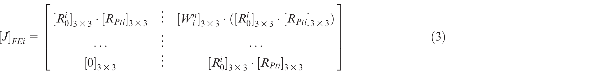
where

where
Moreover, tolerance synthesis and allocation for the J-T model in a deterministic (worst case) solution has been researched primarily. 33 The FR in equation (2) can be seen as the sum of n products for the Jacobian matrix and Torsor model, that is, FR = FR1 + ⋯ + FRi + ⋯ + FRn, (1 ≤ i ≤ n). FRi is obtained as equation (5)
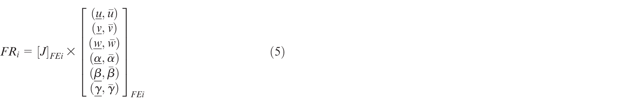
Then, any FE’s percent contribution is equal to

Equation (6) is the deterministic (worst case) method to work out the percent contributions for this model. However, sensitivities of the unified J-T model are not available because of the nonlinear relation between the FR and FEs.
Assembly algorithm
In this article, simplified cylindrical components were adopted to demonstrate the assembly algorithm, where reference 0 was the global reference frame and the turntable axis was designated with a virtual centerline passing through the first component’s base center and was perpendicular to its undersurface, as shown in Figure 1.
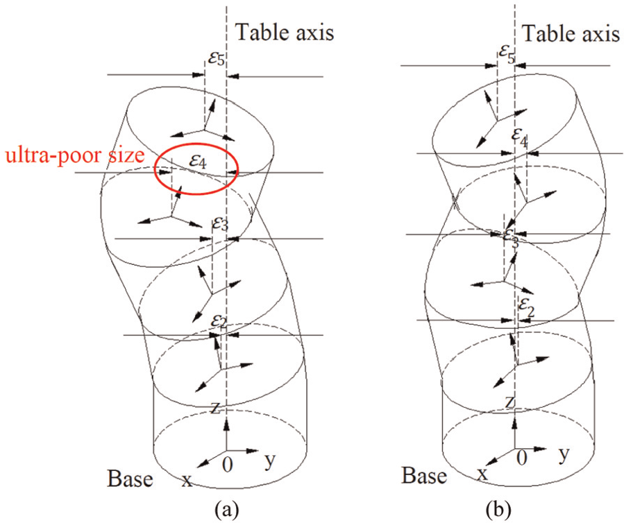
Stackup assembly: (a) top-stage optimization and (b) multistage optimization.
Before using the model, one thing to note is that for simplicity’s sake, a couple of assumptions are made for each component:
In order to eliminate the partial parallel connections structure which could not be generally solved by the Jacobian matrix, contact pairs of the cylindrical joint (A: the locating spigot round) of the rotor parts are ignored, and contact pairs of the planar joint (B: the flange plane) are reserved, as shown in Figure 2(a). In fact, because the mounting surface area of B is much larger than A, the contact pairs of B will play a major role in FR.
In order to contain and simplify the geometric tolerance information, this article uniformly uses the scheme that the bottom surface of each cylinder is designated as the datum, and the top surface is specified by a profile tolerance with the corresponding datum plane, as shown in Figure 2(b).
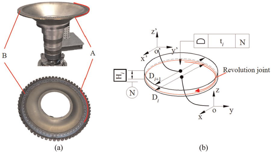
The rotor parts: (a) the actual parts and (b) the geometric model.
Based on the above conditions, the concept of revolution joint (Figure 2(b)) was introduced which is endowed on the bottom surface of each component with no tolerance information. This will lead to the tolerancing torsors of each revolution joint to be zero. The revolution joint essentially belongs to a type of CFE pair used in the Jacobian matrix, and it possesses the rotary regulating effects in the assembly model. More details and the expression about the revolution joint will be demonstrated in section “Solution.”
In order to figure out the optimal solution for the concentricity deviation in overall assembly, more attention is paid on the concentricity deviation of every stage component, rather than that of the top-stage component only. This is because even if the concentricity of the final component is qualified, as shown in Figure 1(a), the concentricities of the former stage components may be dimensionally out of tolerance. Thus, in this work, the target eccentricity of the multistage components (Figure 1(b)) in the complete assembly will be adopted as the whole quality measure, rather than that of the top-stage component (Figure 1(a)).
Multistage rotational optimization is defined as equation (7), that is, the root sum square (RSS) of eccentricities, to control the concentricity deviation of every stage component

where εi is the ith component’s concentricity deviation (i = 2, 3, …, n). Subscript starts from 2 just because the eccentricity calculation starts from the second component.
Therefore, the minimum concentricity deviation of the overall assembly can be obtained at each stage.
Solution
Figure 3(a) has shown a two-stage assembly of cylinders. Three local coordinate systems (1, 2, 3) and the global coordinate system (0) are built in the center of each relevant surfaces. The top surface of each cylinder is specified by a profile tolerance ti (i = 1, 2) with a corresponding datum. The FR is the multistage eccentricity as mentioned in equation (7). For a two-cylinder assembly, it is just the accumulative tolerances on the upper surface of cylinder b along the eccentric direction, which is detected in the global coordinate system.
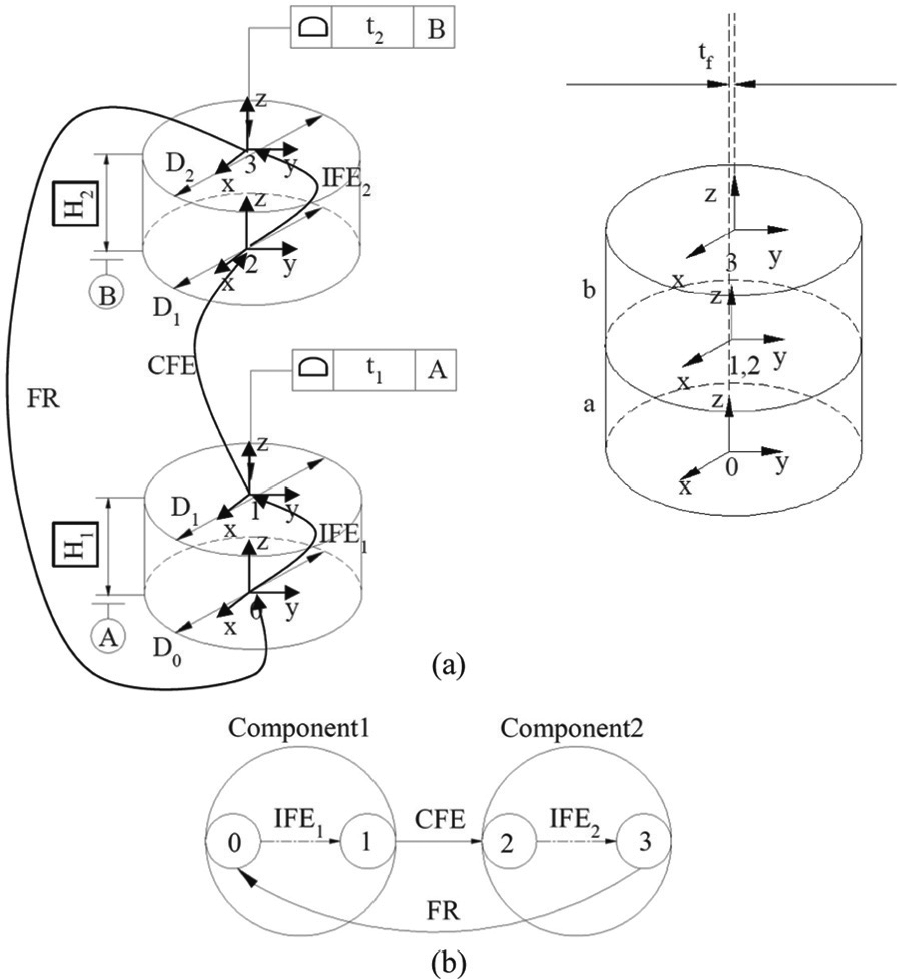
Two-stage assembly: (a) a two-cylinder assembly and (b) connection graph of the two-cylinder assembly.
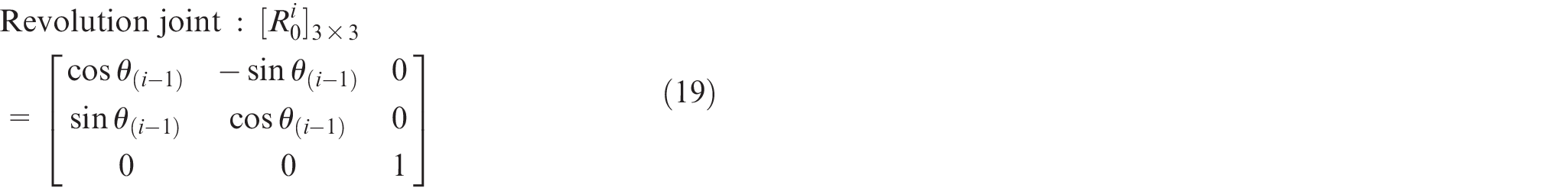
Three FEs shown in the connection graph of Figure 3(b) are two IFEs and a CFE which contains the revolution joint. For the rotationally axisymmetric assembly, the final assembly results will be improved by revolving the components around their symmetric axes, and then the best quality of overall assembly will be received by an appropriate selection of orientation angles for each component. If component 2 is made to rotate by an angle θ1 around the Z-axis, the local orientation matrix

With regard to
Unlike the tolerance zone tilted situation which needs to designate each unit vector on its local axis for tolerance zone tilted based on the tolerance analytic direction, the projection matrix
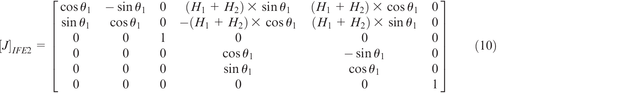
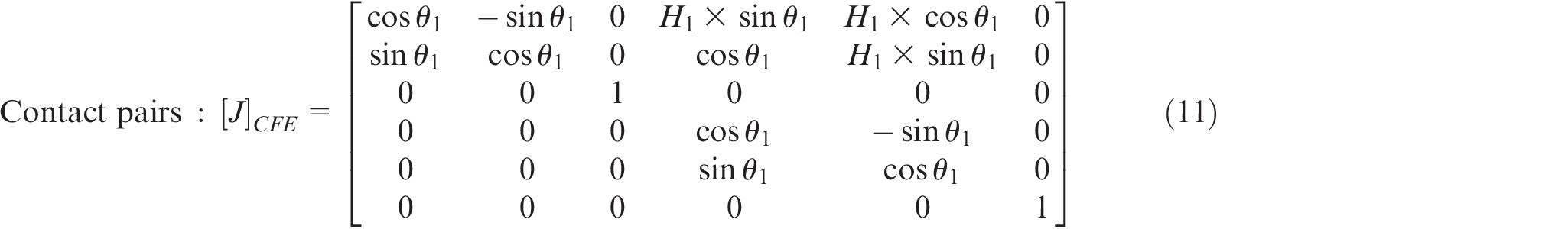
Therefore, the final expressions for the Jacobian matrix associated with the specified internal pairs and contact pairs become
As shown in Figure 2(b) and Table 1, the top surface of each cylinder has three invariant degrees, which indicates that there are three remaining effective vectors in the Torsor model. Roy and Li 51 have given a mathematical derivation of the torsor variations in detail. The torsor variations of each component’s top end can be written as
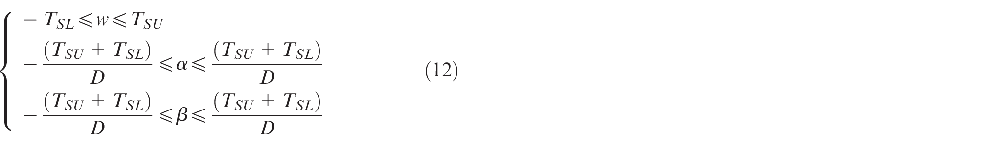
where w is the translation vectors along the z-axis in local reference system; α and β are the rotating vectors around the x- and y-axes, respectively. TSL and TSU are the lower and upper limit values of the profile tolerance. D denotes the cylinder diameter.
Utilizing the Jacobian matrix derived above, relationships among the small displacement torsors of the FRs and all FEs with intervals can be built. That is, deviation propagation function for the two-stage components assembly can be constructed as equation (13)
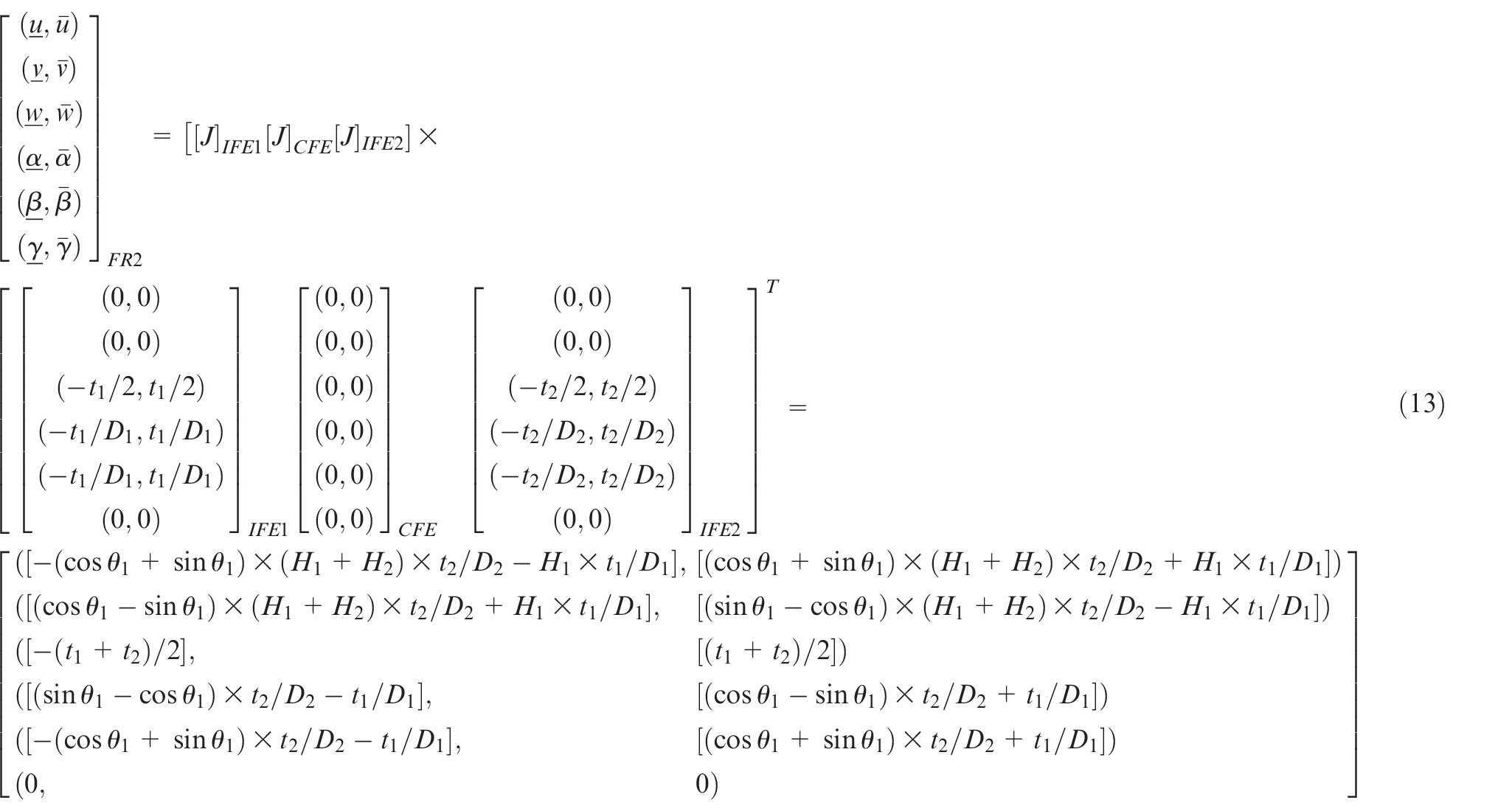
The concentricity deviation interval on the upper end surface of the second cylinder can be determined by means of
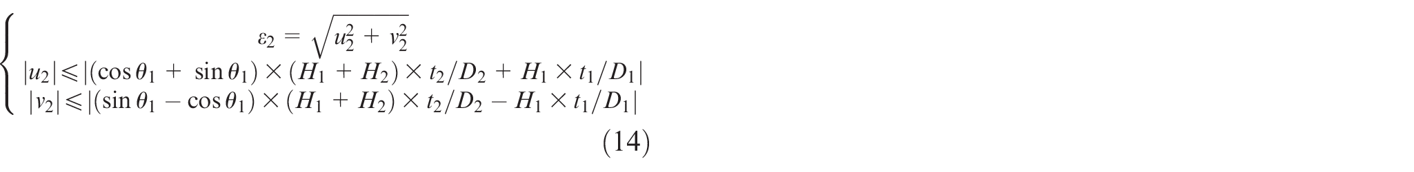
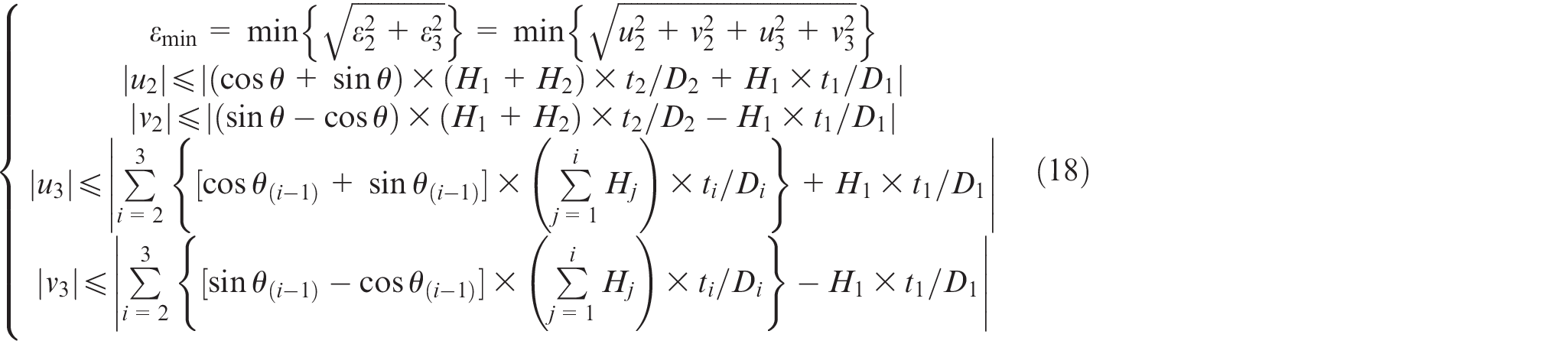
According to equation (7) that has been defined in section “Assembly algorithm,” the multistage optimization expression for two cylindrical components assembly can be calculated as follows
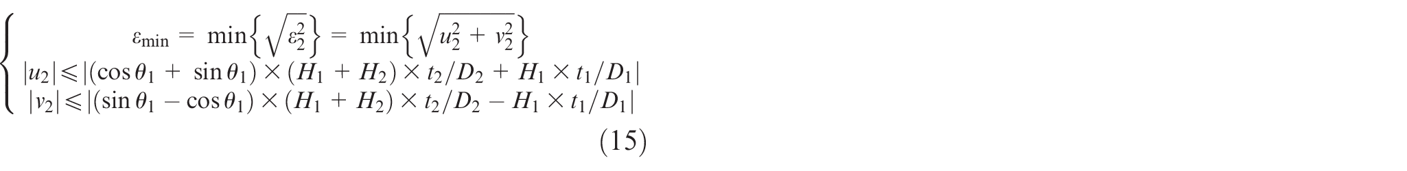
Up to now, the eccentricity expression, inequality constraints, and the objective function of two-stage components assembly have been derived.
Furthermore, three-stage components assembly is studied on the basis of above study. A three-cylinder assembly is shown in Figure 4(a). In order to obtain qualified assembly, component 2 is made to rotate by an angle θ1 and component 3 is made to rotate by an angle θ2 around the Z-axis, respectively, relative to the global reference system.
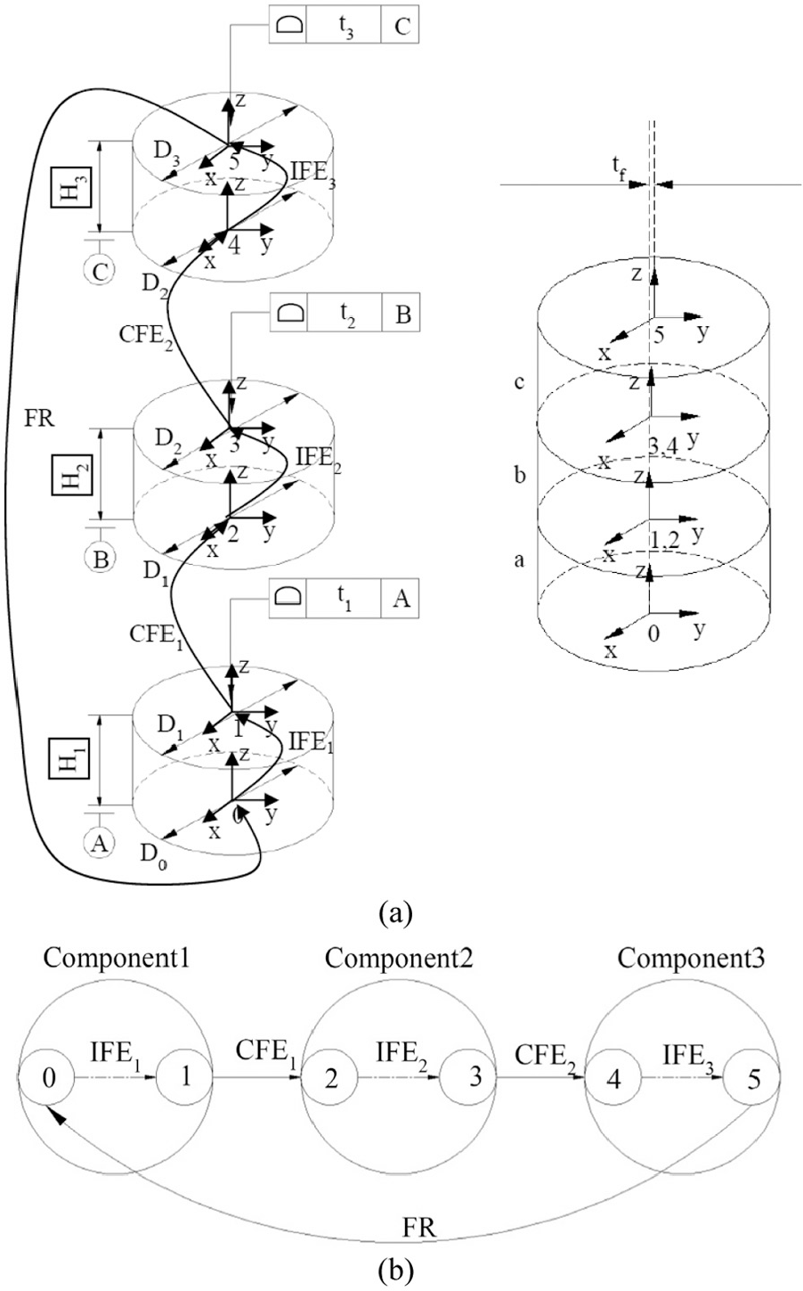
Three-stage assembly: (a) a three-cylinder assembly and (b) connection graph of the three-cylinder assembly.
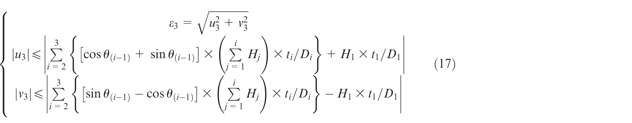
Figure 4(b) is the connection graph of the three-cylinder assembly, similar to the Figure 3(b), including three IFEs and two CFEs. All coordinate systems are located at the center of the tolerance zones or the contact zones. Modeled on equations (8)–(15), the final expression of deviation propagation function for the three-stage components assembly is as follows
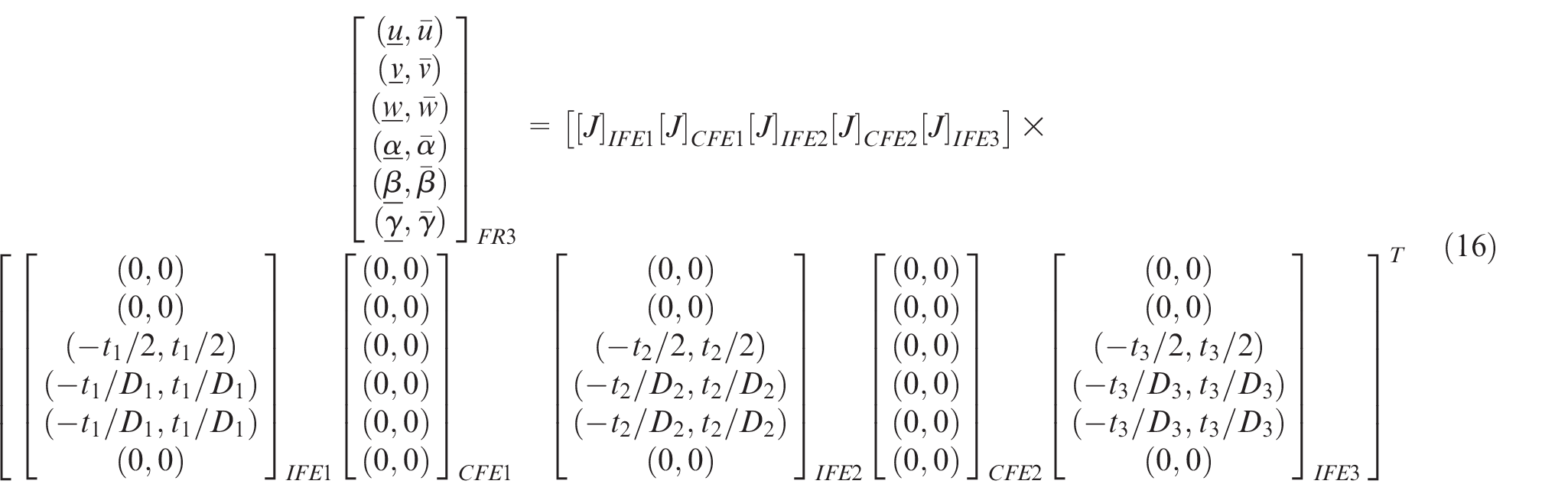
The concentricity deviation interval on the upper end surface of the third cylinder can be determined by means of
Through analyzing the two- and three-stage components assembly, a set of general formulas for the n-stage revolving axisymmetric components assembly can be analytically derived. The general solution of deviation propagation function, inequality constraints, and the objective function can be constructed as follows.
The n-cylinder assembly drawing and the connection graph can be obtained first, which are not repeated here. There are nIFEs and (n - 1) CFEs which represent the rotation effects within the n-cylinder assembly. In order to obtain qualified assembly, component i can be made to rotate with the angle θ(i - 1) around the Z-axis relative to the global reference system. The general local orientation matrix
The FR is the top surface’s accumulative tolerance at the center of local coordinate system n along the eccentric direction which is measured in the global coordinate system.
Based on the above analysis of the two- and three-stage components assembly, the final Jacobian matrix expressing the relationships between the small displacements of the FRs and all FEs can be obtained as equations (20) and (21)
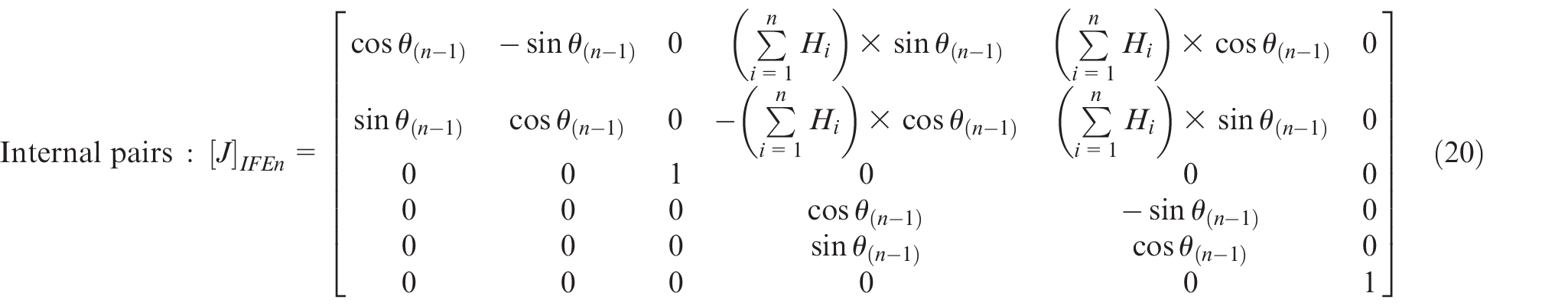
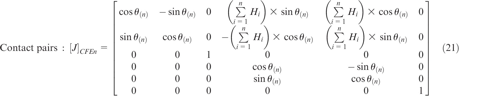
where Hi is the ith component’s height; θi is the (i + 1)th component’s installation angle relative to the global reference system.
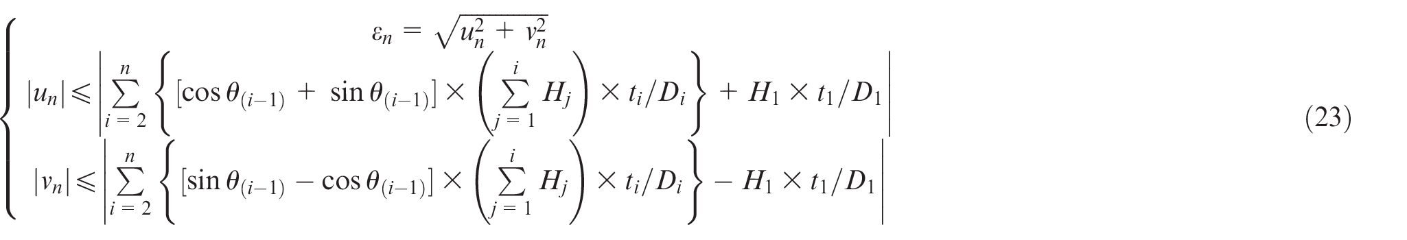
Therefore, the final expression of deviation propagation model for the n-stage components assembly is as follows
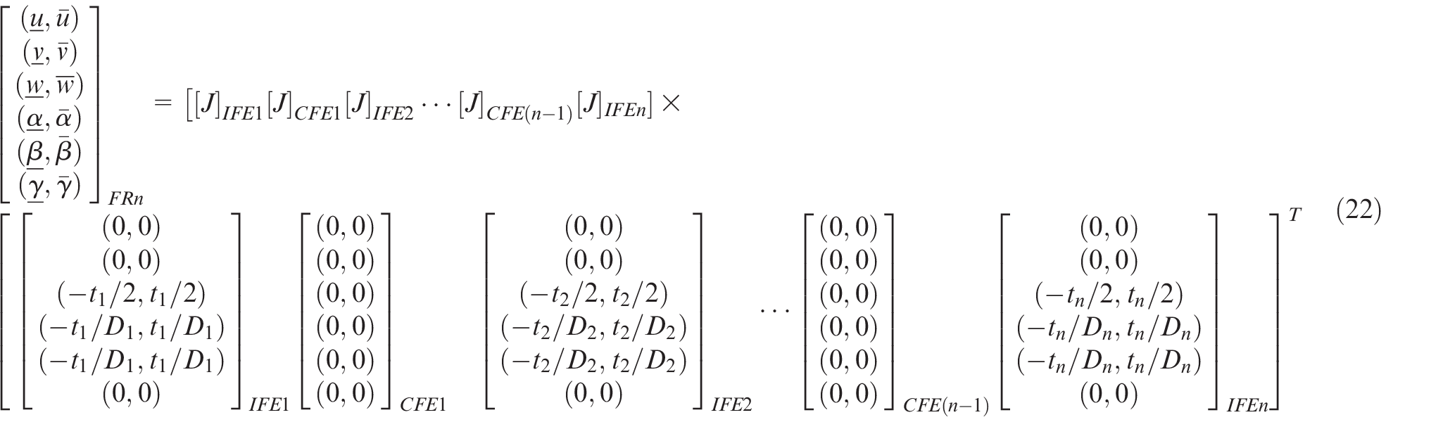
where tn is the nth component’s geometric tolerance that is indicated by a profile tolerance with a datum. Dn is the nth component’s cylinder diameter of its top end (i = 1, 2, …, n).
By far, the
The general multistage rotational optimization expression for revolving axisymmetric components assembly can be derived as equation (24), based on the definition of equation (7)
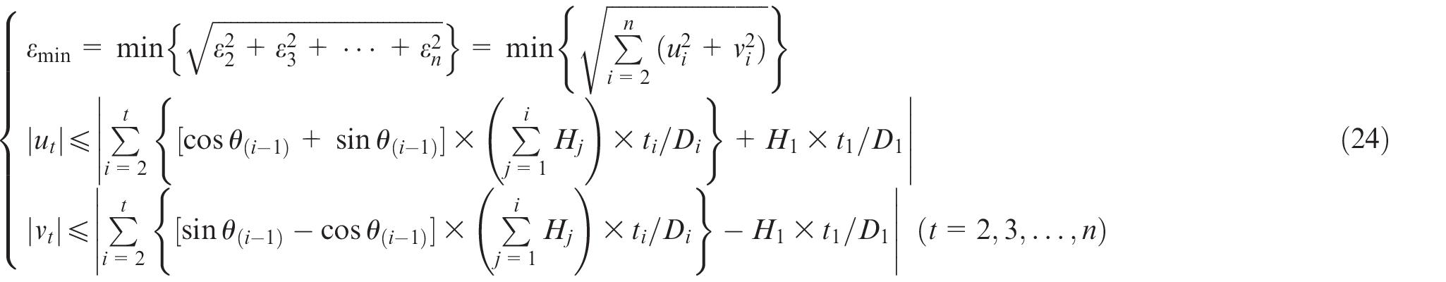
where all the parameters are the same as equation (22).
The general formulas for the n-stage revolving axisymmetric components assembly have been identified, including the expression of deviation propagation model and the multistage rotational optimization function. If the parts deviations are determinate, a unique eccentricity value can be derived. Optimal installation angles of every stage components can be identified using some optimization algorithms. Details on the deterministic (worst case) approach of multistage rotational optimization will be demonstrated in section “Case study.”
Case study
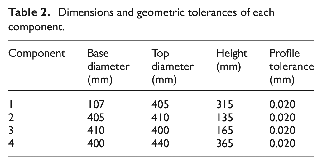
To validate the solution of assembly technique of multistage rotational optimization based on the deterministic (worst case) approach, a realistic subassembly originating in an aero-engine is adopted to prove the application of this method. Figure 5 shows an aero-engine subassembly that was composed of four distinct axisymmetric components, and Table 2 lists the adopted dimensions and simplified geometric tolerances illustrated in Figure 2(b) for each component.
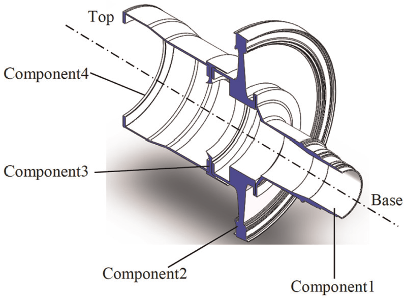
Schematic drawing of four non-identical components assembly.
Dimensions and geometric tolerances of each component.
Based on the multistage assembly algorithm proposed in the previous section, the solving procedures include the following steps:
Step 1. Establish the unified J-T model. In this case, the global coordinate system (0) is set in the base middle of the component 1, and the other local reference frames are built in the center of related contact surfaces. The available IFEs and CFEs are similar to those of three-stage components assembly which have been illustrated in Figure 4(b).
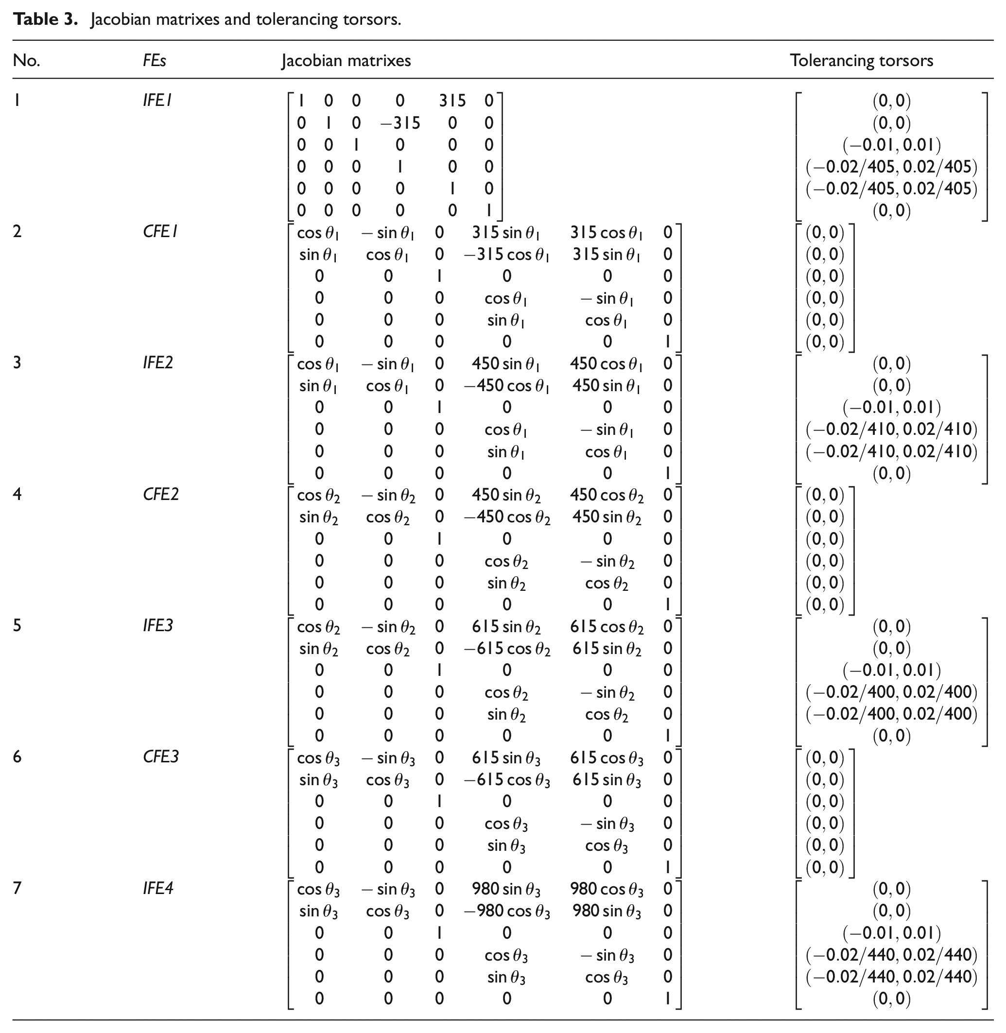
The unified J-T model is built based on the above connection graph. The propagating relationship is IFE1-CFE1-IFE2-CFE2-IFE3-CFE3-IFE4. The Jacobian matrixes and corresponding tolerancing torsors are presented in Table 3.
Step 2. Obtain the final J-T expression and the multistage rotational optimization formula. The expression of the concentricity deviation for the final component is obtained by the proposed method, which can be written as

Jacobian matrixes and tolerancing torsors.
According to the multistage rotational optimization technique presented in this article, the optimization function for this aero-engine assembly can be written as
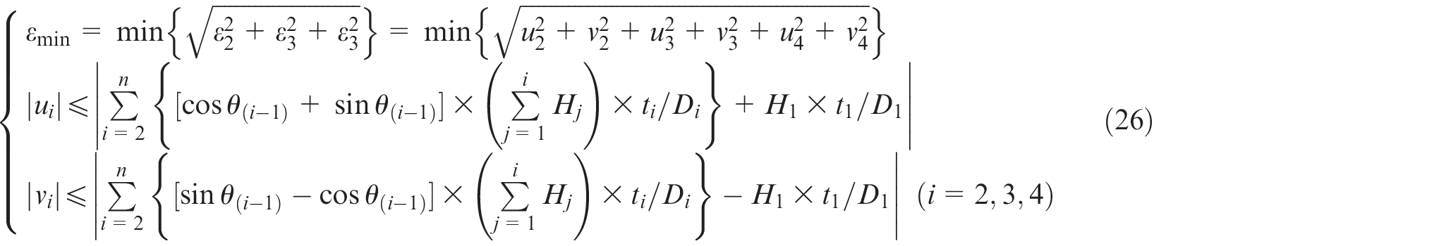
Step 3. Bring up optimum design of the multistage aero-engine assembly. Take the values shown in Table 2 into equation (26) and use a deterministic (worst case) way which has been studied in Ghie et al. 33 to compute the results of ε. Multi-objective genetic optimization algorithm 52 is adopted to acquire the εmin and the optimization procedure is realized by a program. Figure 6 shows the relationship between the target eccentricity (equation (7)) and installation angles of four-stage components.
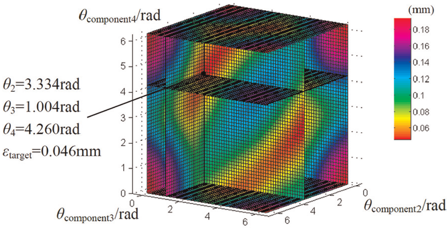
The relationship between concentricity and three installation angles.
The radians of installation angles for the second-, third- and fourth-stage component are on the three mutually perpendicular planes, and the intersection of three variables with the facets indicates the target eccentricity. The colormap represents the value of target eccentricity. As shown in Figure 6, the minimum value of target eccentricity (0.046 mm) can be obtained when the three installation angles are 3.334 rad, 1.004 rad, and 4.260 rad, respectively.
In the same way, the relationship between the target eccentricity and installation angles for the three-stage aero-engine assembly can be calculated and is shown in Figure 7.
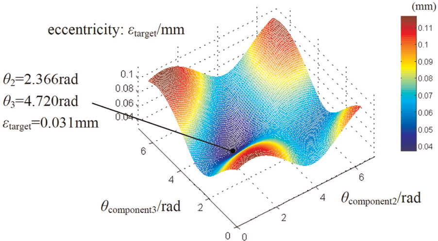
The relationship between concentricity and two installation angles.
The radians of installation angles for the second- and third-stage component are on the two mutually perpendicular horizontal coordinate axes, and the vertical axis indicates the target eccentricity. The colormap visually represents the value of target eccentricity. As shown in Figure 7, the minimum value of target eccentricity (0.031 mm) can be obtained when the two installation angles are 2.366 rad and 4.720 rad, respectively.
Step 4. Analyze the results of εmin. In order to validate the feasibility and efficiency of the addressed technique, the multistage optimization results and the top-stage optimization results are provided in Table 4, together with the results of no optimization.
Concentricity variation for a multistage aero-engine assembly.
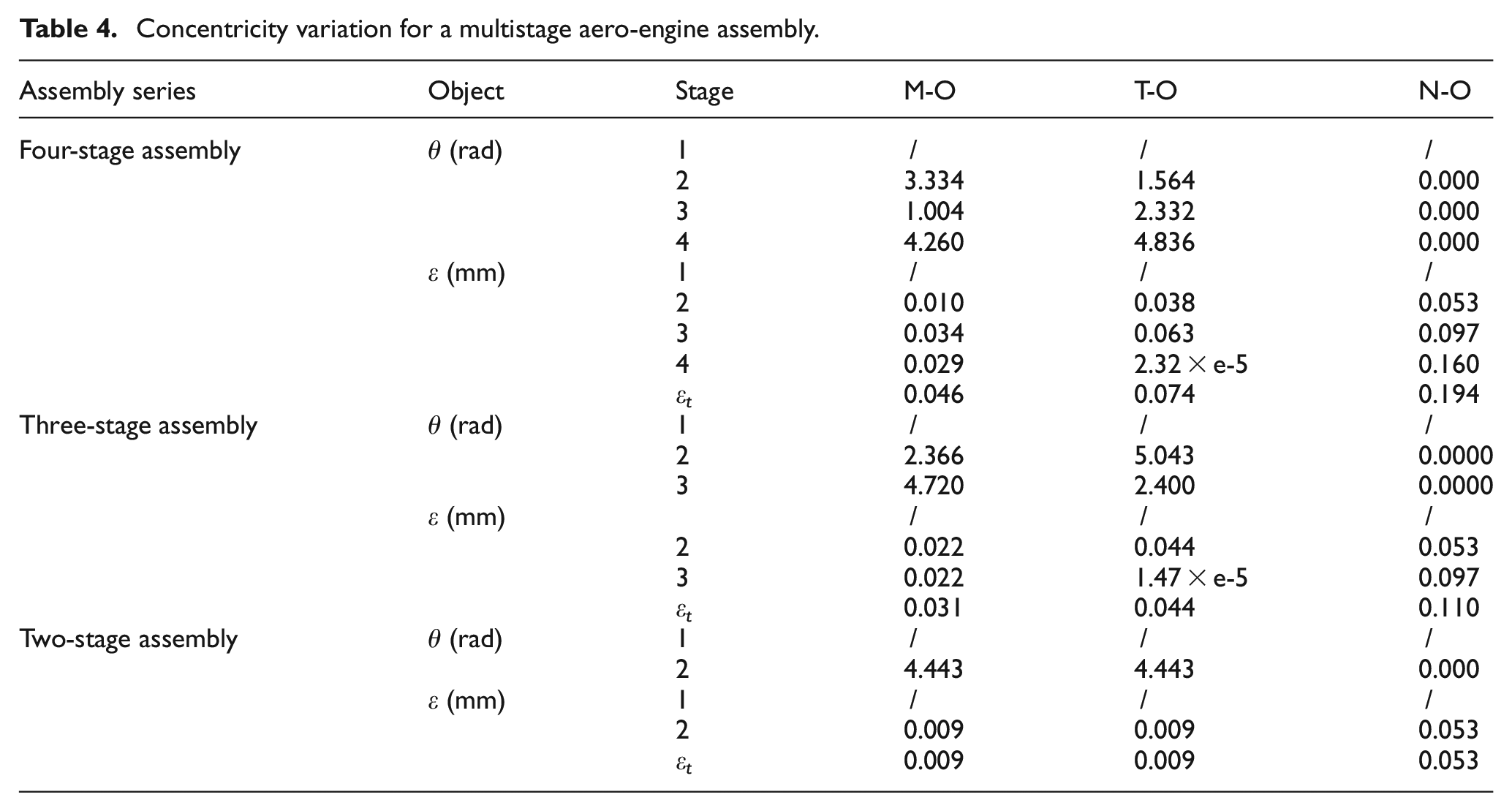
In Table 4, θ is the rotating angle and ε is the eccentricity; εt represents the target value of eccentricity referred in equation (7). M-O, T-O, and N-O are short for “multistage optimization,”“top-stage optimization,” and “no optimization,” respectively.
Likewise, according to step 1 to step 4, the optimization results of the same example for two- and three-stage aero-engine assembly can be obtained in Table 4 as well.
Results and discussion
Key technology and comparison
The results of Table 4 are illustrated in Figure 8. For a four-stage rotors assembly, its target concentricity value has been improved by 76.3% when adopting the multistage rotational optimization, relative to directly assembling with no adjustment. In the same way, the concentricity value is improved by 81.1% at stage two, 64.9% at stage three, and 81.9% at stage four, respectively, compared to the no optimization assembly.
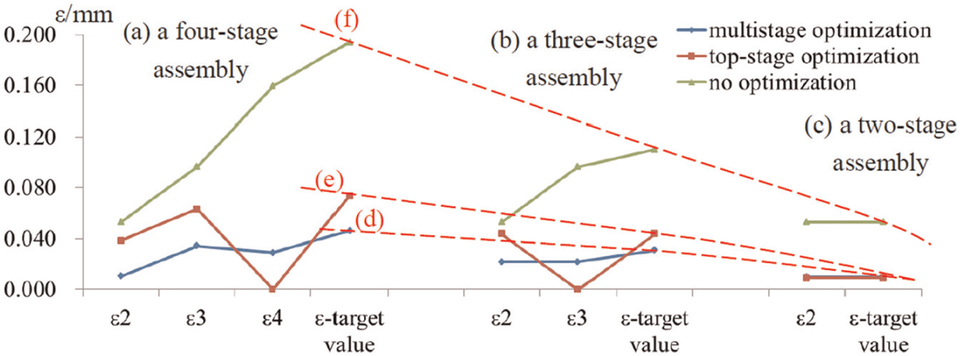
Aggregated eccentricity results of multi-/top-/no-stage optimization.
As expected, the three-stage rotors assembly and the two-stage rotors assembly have similar results to those in the four-stage case. The concentric performances are improved by the technique of multistage rotational optimization at each stage, as shown in Figure 8 and Table 4. For instance, for three-stage rotors assembly, it is improved by 58.5% at stage two, 77.3% at stage three, and 71.8% at the target stage (defined in equation (7)), respectively, compared to the no optimization assembly.
Overall, the above results have a good agreement with those for any multistage components assembly. It indicates that the proposed assembly technique of multistage optimization is valid and effective, and can be implemented in manufacturing processes.
As described in the section “Assembly algorithm,” top-stage optimization is not an effective way to control the overall components concentricity. It is illustrated in Figure 8 where the final stage concentricity can be guaranteed at all cost of other stage concentricity. For instance, for four-stage rotors assembly, by top-stage optimization, the concentricity of the fourth component has shown outstanding performance with almost zero eccentricity; however, the concentricity of all the other stages is worsened. The concentricity is degraded by 73.7% at stage two, 46.0% at stage three, and 60.9% at the target stage, respectively, compared to the multistage optimization assembly. Similarly as shown in Figure 8(b), the result of three-stage rotors assembly has also proved this point.
Based on the above analysis, the overall concentricity performance of aero-engine assembly must be taken into consideration rather than the single performance of the top-stage component only. The assembly technique of multistage rotational optimization can effectively prevent a banana-shaped result (Figure 1(a)) when components deviations are measured and determined. Generally speaking, this novel optimization technique can be used to evaluate the overall assembly performance, and optimize the assembly scheme on the basis of existing tolerance proposal. In aero-engine assembly, it guides for operating personnel to search the optimal installation angles in advance.
In addition, from Figure 8(a)–(c), a further conclusion can be drawn that concentricity control tends to be difficult with the number rise of components. In multistage optimization results (the red dashed line (d)), the target eccentricity value is 0.009 mm of two-stage assembly, 0.031 mm of three-stage assembly, and 0.046 mm of four-stage assembly, respectively. It is observed that with the increase in the stages, the overall concentric performance has declined markedly. The general trend also appears in the process of top-stage optimization assembly and no optimization assembly, as shown by the red dashed line (e) and (f) in Figure 8. These results indicate that concentricity control is essential, and the assembly technique proposed in this article is significantly effective.
It is interesting to note that the approximate slope of line (d) is a minimum, line (e) comes second, and line (f) is the steepest. It further illustrates this new control method has fairly good robustness and consistency.
PC analysis
As previously mentioned, the presented model can be used for contribution analysis. The PCs of seven FEs can be calculated according to equation (6). Take the optimal values of rotating angles θi (i = 2, 3, 4) which have been worked out in the “multistage optimization” column of Table 4, into Table 3 and equation (22) to compute the FRis and FR. FRis and FR here are expressed as

The derived contributions and accumulative percentage contributions (APC) have been normalized and illustrated in Figure 9 in the order of their extents. The results are very useful for tolerance synthesis and optimization of the aero-engine design.
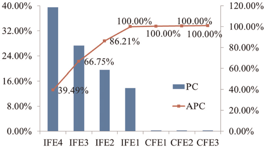
Percentage contributions of seven FEs and their accumulative percentage contributions.
The calculated PCs above have shown that in the four-stage aero-engine assembly, the IFE4 and IFE3 are the contributors of the most important significance. The sum of these two FEs’ contributions is up to 66.75%. It also means that the tolerance of the top-stage component is most sensitive to the FR. Therefore, tightening the first two FEs’ tolerances and relaxing the rest of FEs’ tolerances will be an effective method to achieve a balance between the cost and quality of aero-engine manufacturing. One thing to note here is that the revolution joints are not endowed with any tolerance information; thus, all the PCs of CFE feathers are zero in this case, as shown in Figure 9. As a base for preliminary study, this article just considers that the revolution joints of CFEs only possess rotary regulating effects in the model.
Experimental study
The analysis on accuracy and reliability was made with the experimental results. As shown in Figure 10, a group of aero-engine rotors coupled on the same rotary main axis of the air-bearing turntable. Their structures, dimensions, and tolerance specifications were similar to the case in the previous section, where the parameters were omitted for confidential reasons. A radial dial indicator was used to measure the run-out value of the final component flange, and an axial dial indicator was used to measure the run-out value of the end face. The former was applied to characterize the concentricity, and the latter was adopted to control tilt amount.
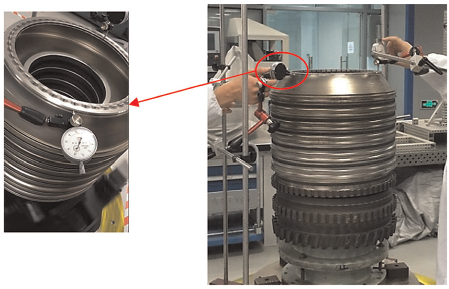
Adjustment and measurement of the experiment.
With the rotors assembled randomly without optimization, the measured data of radial run-out was 0.092 mm. It was hardly to meet the target requirement (0.050 mm) by manual adjustments. While using the assembly technique of multistage rotational optimization which has been described in this article, it took nearly 3 h to acquire the radial run-out of 0.043 mm. Comparative results showed that this assembly technique was conducive to deviation propagation control for revolving components assembly, and of high practicability. It could be integrated with the CAD systems to provide aid for operators in the arduous task of aero-engine assembly.
Conclusion
This work was attempting to propose a novel assembly technique for concentricity control in aero-engine assembly. The revolution joint was introduced in the J-T model for multistage rotational optimization, and a calculating scheme was illustrated on a realistic case originating in aero-engine subassembly. Following conclusions could be drawn:
For a four-stage components assembly, the minimum value of target eccentricity (0.046 mm) can be calculated when the three optimal installation angles (3.334 rad, 1.004 rad, and 4.260 rad) are searched. This assembly technique can be integrated with the CAD systems to provide aid for operators in the arduous task of aero-engine assembly.
Using multistage rotational optimization technique, the overall concentric performance has improved 60.9% relative to the top-stage optimization and 76.3% relative to directly assembling. Experiment results highlighted the benefits that this method was feasible and of high practicability, and could easily predict the final assembly quality.
The derived deviation propagation model can be utilized for assembly tolerances redesign, where each FEs’PCs can be obtained. In the four-stage components assembly, tightening the upper two FEs’ tolerances (APC = 66.75%) and relaxing the lower FEs’ tolerances is an effective way to achieve a balance between the quality and cost.
Moreover, shortcomings for the proposed method are that it cannot well solve the partial parallel chain problem, and deformation of working parts under load would also be difficult to deal with. In future, the rotor structure with the locating spigot round and bolted connection will be considered, to model and optimize the actual assembly process, which can be advantageous to guide assembling fulfillment.
Footnotes
Acknowledgements
The authors are grateful for all the reviewers’ reasonable suggestions on this article’s improvement.
Declaration of conflicting interests
The author(s) declared no potential conflicts of interest with respect to the research, authorship, and/or publication of this article.
Funding
The author(s) disclosed receipt of the following financial support for the research, authorship, and/or publication of this article: This work was supported by the grants from the National Natural Science Foundation of China (Grant Nos. 51121063 and 51175340) and the National Science & Technology Pillar Program during the 12th Five-year Plan Period (Grant No. 2012BAF 06B03).