
Abstract
Line segments, or G01 codes, generated by computer-aided manufacturing softwares are the most widely used toolpath format for computer numerical control systems. The linear toolpath normally consists of thousands of short line segments due to the high-accuracy requirement of the machined parts. Due to the tangential and the curvature discontinuities at the junction of two segments, the feedrates at the start and the end points of line segment have to be slowed down. In order to increase the feedrates along short line segments, a locally optimal transition method is proposed, which uses a two-step strategy to generate a blended toolpath composed of cubic Bezier curves and line segments. In the first step, the optimal proportional coefficient is represented as the function of the angle between two adjacent line segments, which can be employed to minimize the curvature variation energy of the cubic Bezier curve. In the second step, the local optimization model with the aim to minimize the sum of two curvature extrema is established to determine the optimal transition length. The transition length can be analytically obtained under the constraint of the approximation error and the constraints of the line segment lengths. The simulation and experiment results demonstrate that, by comparison with the conventional transition methods, the proposed method can significantly decrease the machining time but does not increase the contouring error.
Keywords
Introduction
With the development of part design and manufacturing technologies, high-feedrate and high-accuracy machining is increasingly required by complex parts such as die-molds, turbines, impellers, and aerospace components. 1 The toolpath generated by computer-aided manufacturing softwares is often represented by short line segments.2,3 Due to the tangential and the curvature discontinuities at the junction of two line segments, the feedrates at the start and the end points of the line segment have to be slowed down to avoid the feedrate fluctuation and the acceleration oscillation. 4 Recently, some commercial computer-aided design (CAD)/computer-aided manufacturing (CAM) softwares have developed the capability of generating numerical control (NC) codes in a parametric format. However, vast majority of computer numerical control (CNC) systems still accept toolpaths represented by line segments rather than parametric curves. Therefore, it is necessary to smooth line segments in order to improve the machining efficiency.
To generate smooth motion along linear toolpath, two major methods, that is, fitting methods5–7 and transition methods, have been proposed. The fitting methods utilize interpolation or approximation technique to generate continuous toolpath from G01 codes. They have been adopted by some advanced commercial CNC systems.8,9 However, there are three shortcomings when the fitting methods are applied.10,11 First, spline curve may wiggle its way when fitting densely short line segments. Second, the fitting error is difficult to control. Third, the fitting is generally computationally demanding.
The transition methods, called corner smoothing methods, usually employ circle arcs,
12
polynomials,13,14 or free-form curves15–22 to blend adjacent line segments. In the high-order polynomial-based transition methods,13,14 the curvature extremum cannot be analytically obtained and the maximum bound on the deviation of the blended toolpath from the linear toolpath is not considered. Yau and Wang
15
proposed a fast
The proposed transition method consists of two steps. In the first step, the relationship between the optimal proportional coefficient and the angle between two adjacent line segments is established. It can be used to analytically minimize the CVE of the cubic Bezier curve. In the second step, the local optimization model with the aim to minimize the sum of two curvature extrema is established to determine the transition length. The locally optimal transition length can be analytically obtained under the constraint of the approximation error and the constraints of the line segment lengths.
The rest of this article is organized as follows. Section “Preliminary” introduces the preliminary of
Preliminary
A kth-degree Bezier curve 23 is defined by
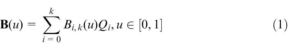
where
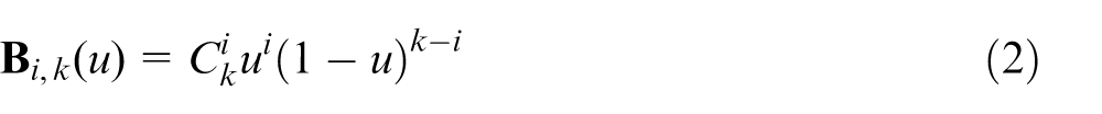
In Zhao et al.,
20
two symmetric cubic Bezier curves
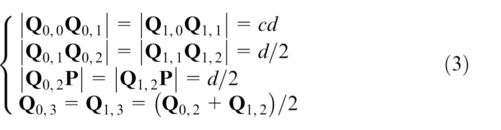
where c is a positive proportional coefficient,
Description of
The curvature extremum
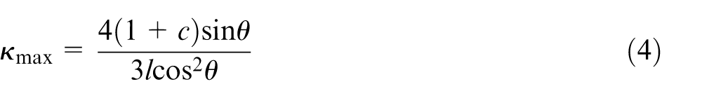
where
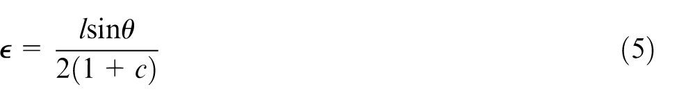
The approximation error
Cubic Bezier curve with minimum CVE
In the design of free-form toolpath, the CVE is invoked as a measure of the smoothness of toolpath due to the fact that high CVE means curvature oscillation. The CVE has the following formula 24
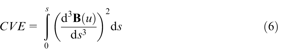
where S is the total arc length of the parametric curve, and s is the arc-length parameter.
According to equation (3), the proportional coefficient, c, in addition to the transition length, l, has an effect on the geometry of the transition curve. Substituting equation (3) into equation (6), the CVE of left cubic Bezier curve
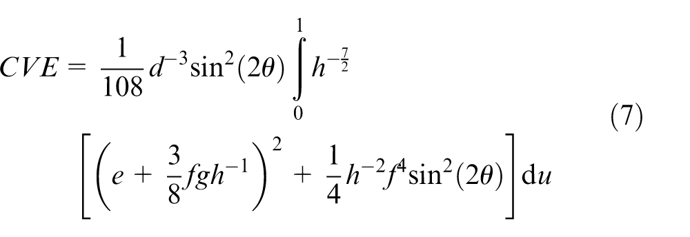
where e, f, g, and h have the following expressions
Note that fixing
CVE changes when the proportional coefficient linearly increases.
With the aid of MATLAB, the function “lsqcurvefit” is used to fit relationship between the optimal proportional coefficient and the angle between two adjacent line segments, and the obtained function
Locally optimal transition method
In this section, a locally optimal transition method with analytical calculation of transition length is illustrated. As depicted in Figure 3,
Application of the locally optimal transition method.
In this article, the sum of the two curvature extrema is adopted as the optimization objective that should be minimized. The local optimization model can be formulated as follows
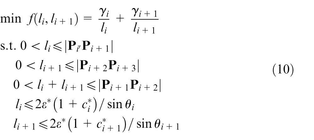
where
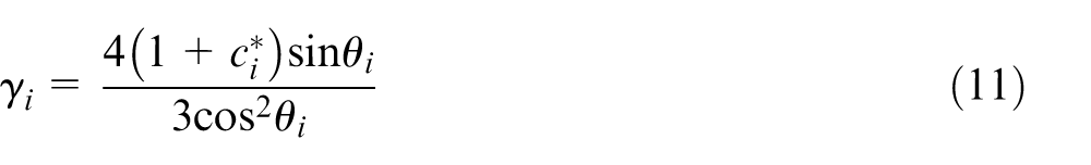
To solve the optimization problem, the initial transition lengths
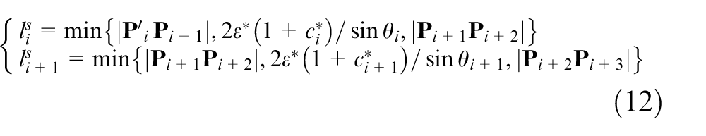
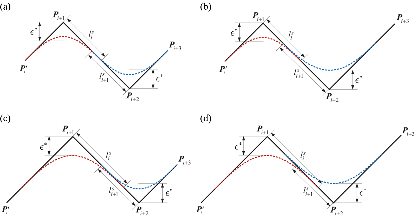
Initial transition lengths
If
However, if
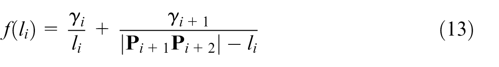
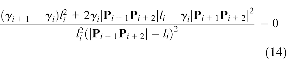
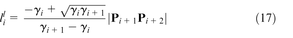
In order to obtain the extremum of
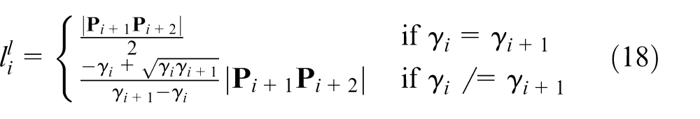
If
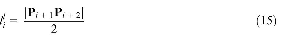
If
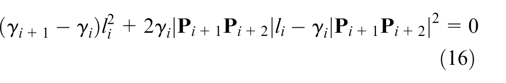
The solution to equation (16) can be analytically determined by the following theorem.
Theorem 1
The quadratic equation
The proof is given in Appendix 1.
As a result, the initial transition length
Note that
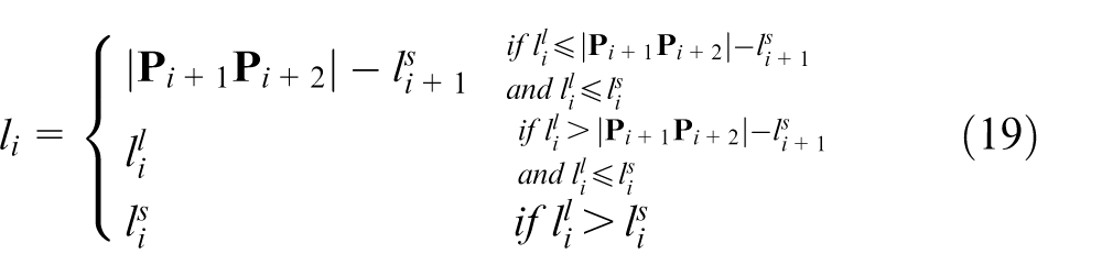
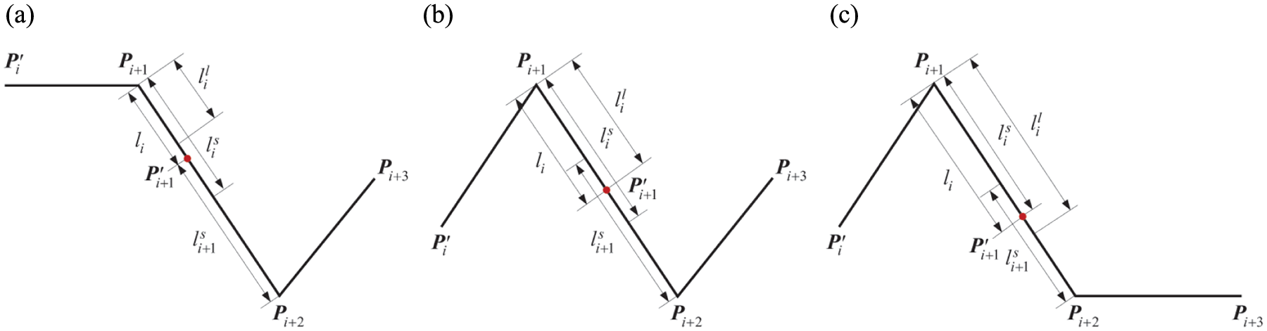
Locally optimal transition length
Obviously, for the short line segments, the actual approximation error of the transition curve is less than the specified approximation error
The transition length is always restricted to be half of the line segment length in the conventional methods. 20 It is locally optimized in the proposed method. Thus, the proposed method can provide a more proper transition length than the conventional transition methods. As a result, the higher feedrate can be achieved for the generated transition curve.
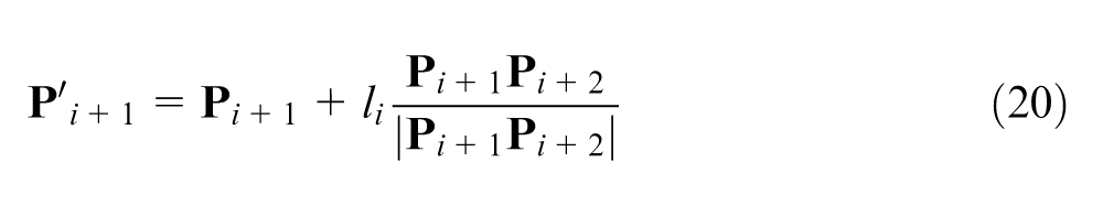
The initial point
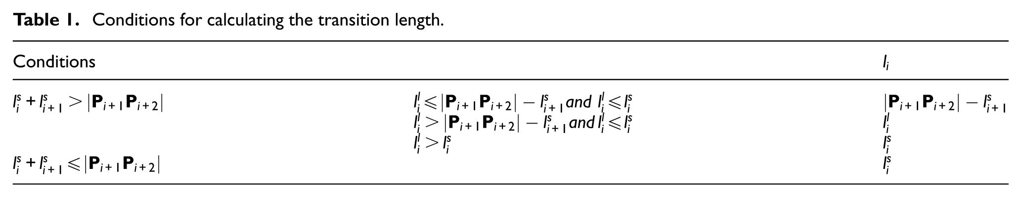
All the conditions for calculating the transition length are summarized in Table 1. Based on the above analysis, we give the following algorithm to analytically determine the locally optimal transition length.
Conditions for calculating the transition length.
Algorithm
LoOpTran
Input. The point sequence
Output.
Step 0
Set
Step 1
Set transition unit
Compute
Compute
Compute
(a) If
(b) If
Step 2
Compute
Compute
Go to Step 3.
Step 3
Compute
Set
(a) If
(b) If
By applying this algorithm, we can smooth the linear toolpath using locally optimal cubic Bezier curves with minimum CVE.
Simulation and experiment
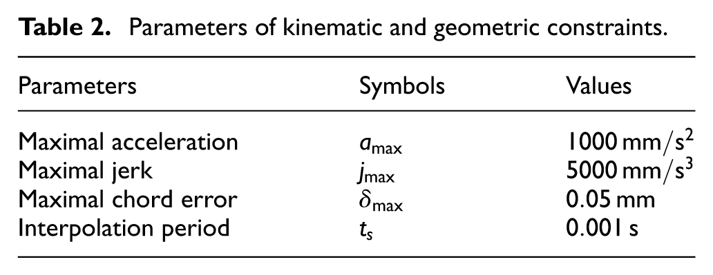
The performance of the proposed algorithm is compared with that of the conventional transition method whose transition length is restricted to be half of the line segment length in Zhao et al. 20 For the sake of conciseness, the proposed transition method and the conventional transition method are abbreviated as “LOTM” and “CTM,” respectively. The jerk-limited feedrate algorithm 25 and the second-order Taylor expansion formula based on the arc length 20 are adopted to generate kinematic profiles and reference position commands, respectively. The locally optimal transition method is coded with VC++. The parameters used in the interpolator are listed in Table 2.
Parameters of kinematic and geometric constraints.
Simulation
In the simulation, the Zigzag linear toolpath, as shown in Figure 6, is utilized to illustrate the effectiveness of the proposed transition method. It is composed of 13 short line segments which are listed in Table 4 of Appendix 2. For fair comparison, LOTM and CTM share the same command feedrate 10 mm/s and the specified approximation error of 0.5 mm.
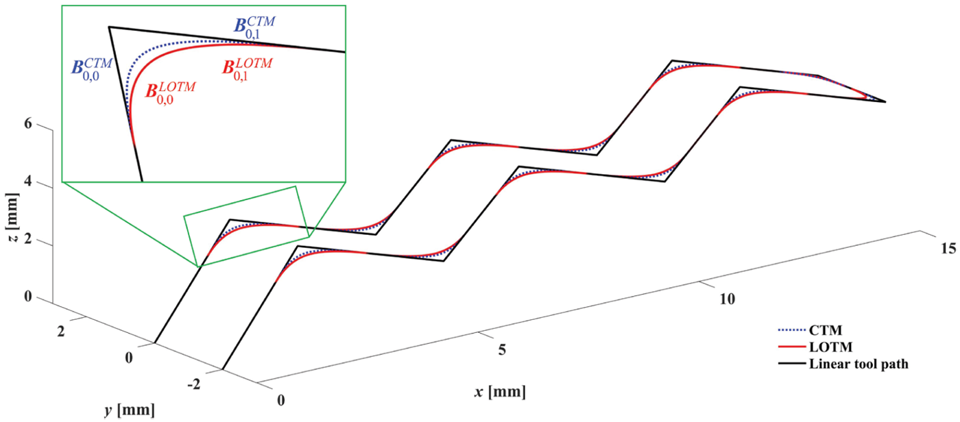
Zigzag linear toolpath.
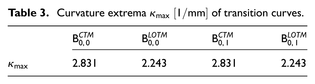
The blended toolpaths with the CTM and the LOTM are denoted by blue dashed lines and red solid lines in Figure 6, respectively. The curvatures of the transition curves within the green solid rectangle in Figure 6 are depicted in Figure 7. It can be observed that the curvature decreases appreciably when the LOTM is applied by comparison with the CTM. As listed in Table 3, the curvature extrema obtained with the LOTM is significantly lower than those obtained with the CT. The kinematic profiles depicted in Figure 8 indicate that the machining time decreases from 4.861 s obtained with the CTM to 4.269 s obtained with the LOTM, decreasing by 12.18%. As analyzed in section “Locally optimal transition method,” the proposed method has higher machining efficiency than the conventional transition method when linear toolpath is composed of the short line segments. The lengths of the toolpath generated by the LOTM and CTM are 44.249mm and 45.850mm respectively. The length by the LOTM is 3.49% shorter. The machining time is decreased mainly due to the increase of the actual feedrate rather than the decrease of the toolpath length.
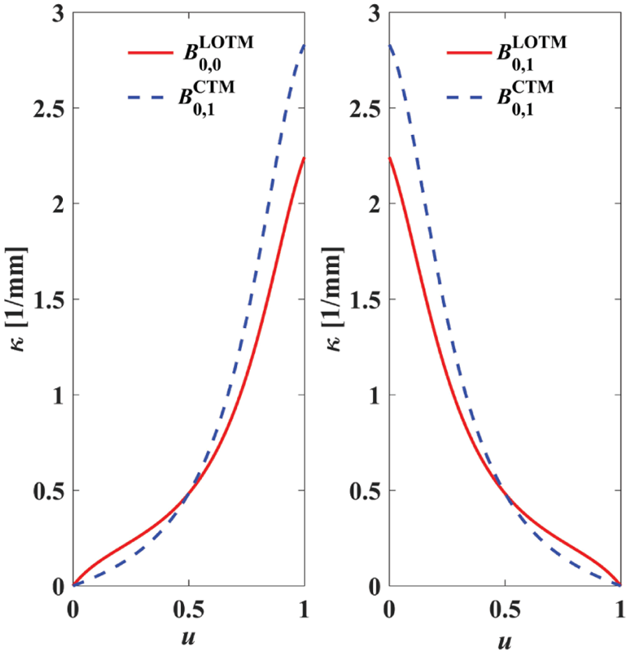
Curvature distributions of transition curves.
Curvature extrema
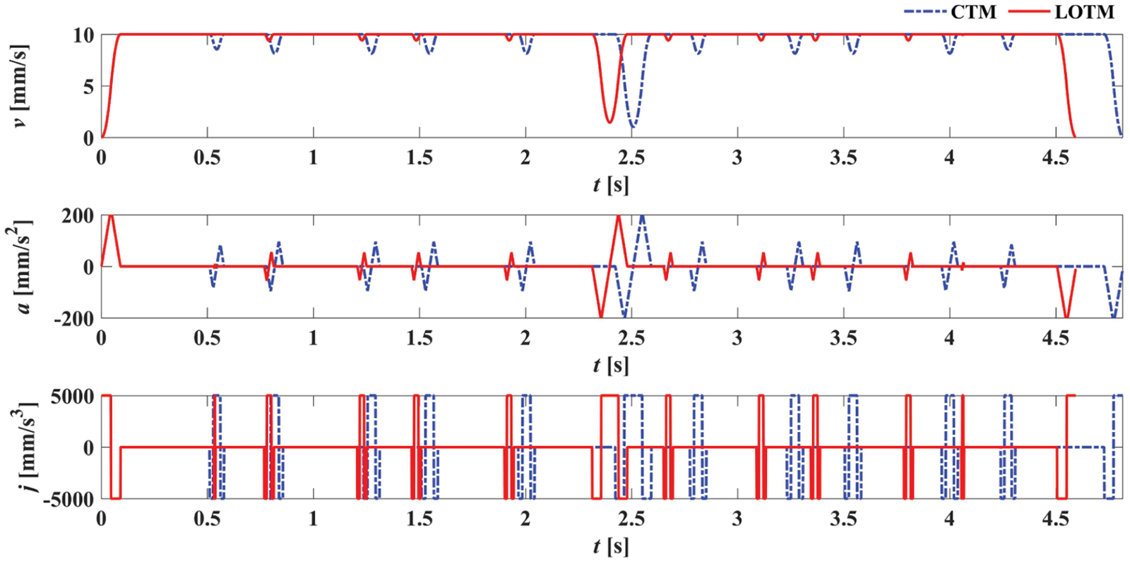
Scheduled feedrate, acceleration, and jerk profiles along the Zigzag toolpath.
Experimental setup
To validate the effectiveness of the proposed transition method, experiment is carried out on a three-axis experimental table driven by YASKAWA SGDV series servo drivers and SGMJV motors, as illustrated in Figure 9. The lead of the ball screw used in the triaxial table is 10 mm/rev, and the resolution of incremental encoder for each motor is 10,000 pulse/rev. Then, the reference position commands generated by the interpolator are sent to the dSPACE-DS1103 system for motion control.
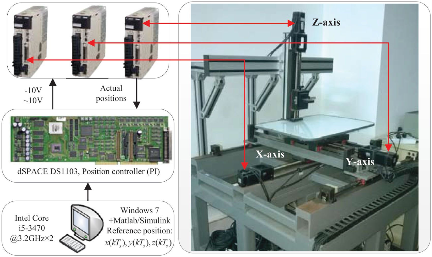
Layout of three-axis experimental table.
Experiment
In the experiment, the Rhombus linear toolpath, as shown in Figure 10, is used to illustrate the effectiveness of the proposed transition method. It is composed of 18 line segments which are described in Table 4 of Appendix 2. The command feedrate and the approximation error are set to be 50 mm/s and 1.0 mm, respectively.
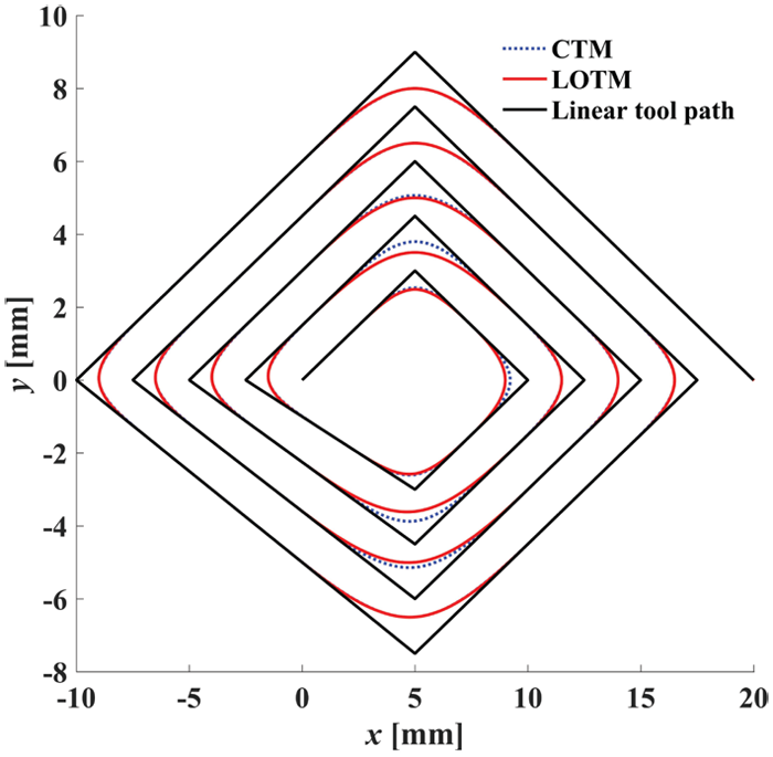
Rhombus linear toolpath.
As depicted in Figures 11 and 12, the kinematic profiles indicate that the machining time decreases from 5.366 s obtained with the CTM to 5.260 s obtained with the LOTM. Note that the machining efficiency in experiment is not improved as significantly as that in simulation. The reason is that Rhombus linear toolpath is composed of long line segments. As analyzed in section “Locally optimal transition method,” the local optimal transition length is determined by the specified approximation error when the linear toolpath is composed of long segments. In the experiments, the contouring error, which is defined as the distance from the actual point to the original linear toolpath, is adopted to evaluate the contour-following accuracy of the CTM and the LOTM. The maximum and the mean contouring errors resulting from the LOTM are 0.5348 and 0.0973 mm, respectively. The maximum and mean contouring errors resulting from the CTM are 0.6904 and 0.0945 mm, respectively. The maximum contouring error with the LOTM is quite smaller than that with the CTM. The mean contouring error with the LOTM is slightly larger than that with the CTM, which is mainly caused by a larger average deviation between the blended toolpath and the linear toolpath with the LOTM, as shown in Figure 13. In fact, the maximum contouring error usually plays a more critical role than the mean contouring error in evaluating the contour-following performance.26,27 Therefore, the proposed method, by comparison with the conventional transition method, can achieve a higher machining efficiency and keeps a similar contour-following accuracy.
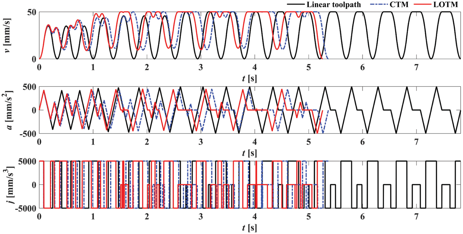
Scheduled feedrate, acceleration, and jerk profiles along the Rhombus linear toolpath.
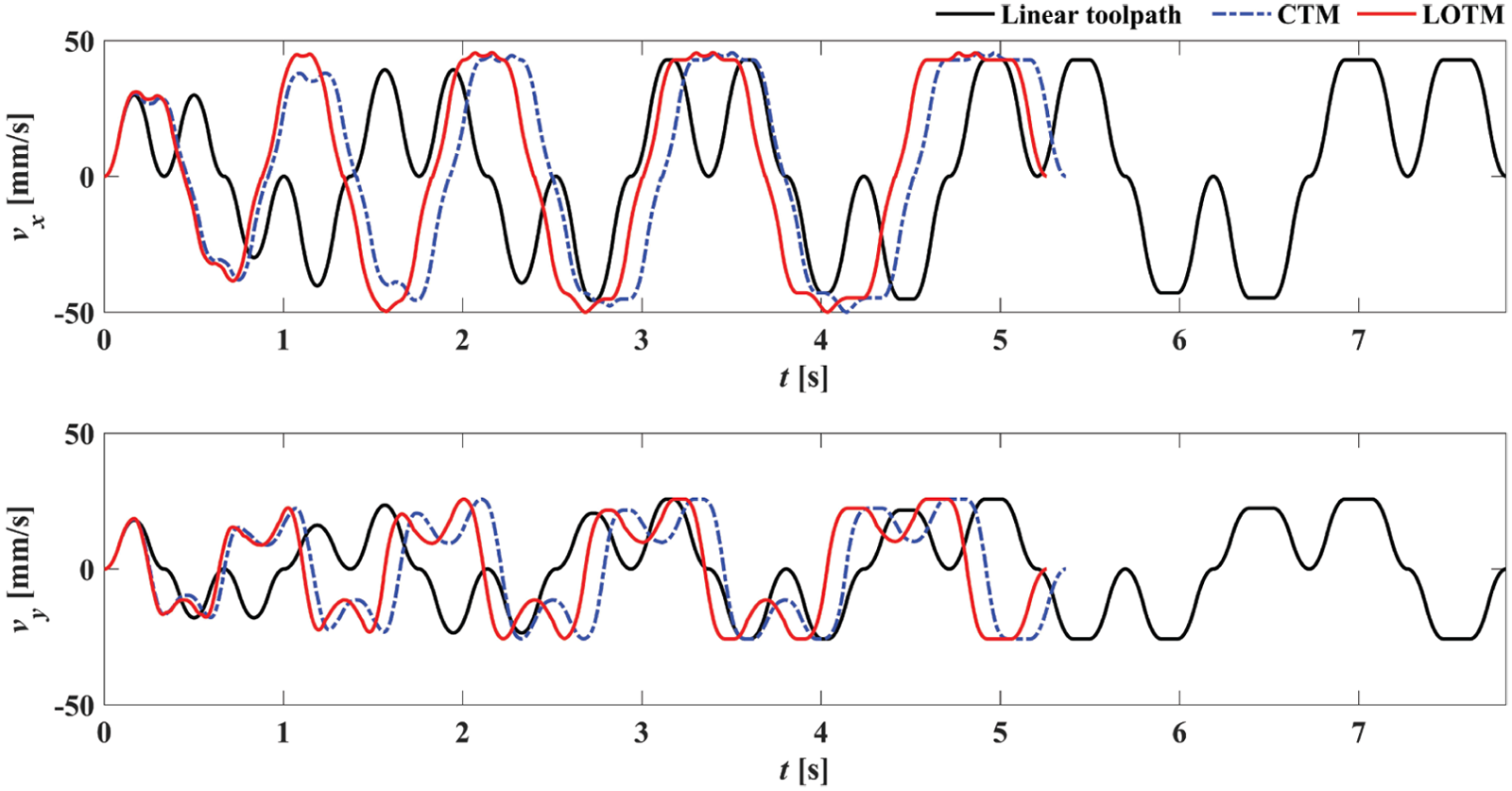
X-axis and Y-axis feedrate profiles.
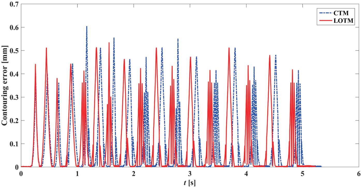
Contouring errors.
Conclusion
In this work, a locally optimal transition method is proposed for CNC machining of short line segments. Compared with the conventional methods with fixed transition length, the proposed method has the following advantages:
The optimal proportional coefficient is represented as a function of the angle between two line segments, which can be used to analytically minimize the CVE of the cubic Bezier curve for transition.
The local optimization model with the aim to minimize the sum of two curvature extrema is established. Under the constraint of the approximation error and the constraints of the line segment lengths, the transition length can be analytically obtained.
The simulation and experiment results demonstrate that the proposed method achieves higher efficiency while keeping a similar accuracy by comparison with the conventional transition method.
Footnotes
Appendix 1
Appendix 2
Declaration of conflicting interests
The author(s) declared no potential conflicts of interest with respect to the research, authorship, and/or publication of this article.
Funding
The author(s) disclosed receipt of the following financial support for the research, authorship, and/or publication of this article: This work was partially supported by the National Natural Science Foundation of China under grants no.51325502 and no.91648202, and the Science & Technology Commission of Shanghai Municipality under grand no.15550722300.