Sage Journals: Discover world-class research

Abstract

Surface roughness is a variable often used to describe the quality of ground surfaces as well as to evaluate the competitiveness of the overall polishing system, which makes it an ever-increasing concern in industries and academia nowadays. In this article, from microscopic point of view, based on the statistics analysis, and by the use of the elastic contact theory and the plastic contact theory, the model of the maximum cutting depth of abrasive grains is developed. Then based on back-propagation neural network, taking the maximum cutting depth of abrasive grains, the rotation speed of belt and the feed rate of workpiece as the input parameters, a prediction model of surface roughness in belt polishing is presented. The prediction model fully takes the characteristics of polishing tool and workpiece into consideration which makes the model more comprehensive. Compared with the model that takes the polishing force as the input parameter, the model in this article needs fewer experiment samples which will save the experiment cost and time. Moreover, it has a wider range of uses and is suitable for different polishing situations such as different workpieces and polishing tools. The results indicate a good agreement between the predicted values and experimental values which verify the model.

Keywords

Surface roughness maximum cutting depth belt polishing artificial neural network statistics analysis

Introduction

Polishing is a kind of finishing process that can effectively eliminate or reduce the processing defects caused by former manufacturing procedures and improve the surface quality and form accuracy, which makes it a vital role to ensure the product quality and the service life.^1,2 Surface roughness is the most widely used index for product quality evaluation and an important variable to evaluate the competitiveness of the overall polishing system. Therefore, the research on surface roughness in polishing has become a hot topic in the field of engineering and academic.^3,4

The polishing process is a complex material removal process involving rubbing, scratching, plowing and cutting between the workpiece and a large number of grains on the surface of the polishing tool. Therefore, there are a number of factors in the polishing process that can affect the surface roughness,⁵ including process parameters such as the tool speed, the feed rate and the polishing force; the characteristics of the polishing tool such as the grain size and material as well as the characteristics of the workpiece such as modulus and curvature. The combined effects of these factors lead to a difficulty in predicting the surface roughness. In practice, the polishing parameters are generally chosen primarily on the basis of human judgment and experience and to some extent on the basis of handbooks, which are highly conservative and does not lead to achievement of optimum polishing parameters and hence loss of productivity and accuracy.⁶ Therefore, it is necessary to perform further studies on surface roughness to achieve a more comprehensive understanding to improve polishing efficiency and quality.

Many scholars have done a lot of work on the research of surface roughness prediction and achieved certain results. The existing roughness prediction models can be divided into three categories: theoretical models, empirical models and intelligent models. Based on the analysis of the interaction between the workpiece and the abrasive grains, theoretical models are developed from microscopic point of view.^7,8 They are applicable to different polishing conditions and thus have a broad scope. While they are mostly based on statistics method which involves a large amount of computations, the calculations are very complicated. In addition, theoretical models are usually based on ideal conditions with a variety of assumptions, resulting in a large deviation between the predicted results and the actual results. In the empirical methods, the relationship between the process parameters and the surface roughness is established based on polishing experiments.^9–11 Compared with theoretical models, empirical models are simple and convenient which do not need complex calculations and profound theoretical knowledge. Since the empirical methods are on the case-by-case basis, a model established under one polishing condition generally cannot be used for other conditions, and hence, the scope of its application is limited.

To overcome the disadvantages of the two methods above and combined with the fact that in many cases surface roughness is difficult or even cannot be described using specific expression, intelligent models have been tried out to predict surface roughness in polishing. Intelligent models are based on the intelligent algorithm. Different from the classical mathematical methods, intelligent models solve complex problems by simulating the natural ecosystem mechanisms. The models are simple and have a wide range of applications. Recently, there has been a lot of interest to develop prediction models for the surface roughness using artificial intelligence techniques.^6,12–14 The main intelligence models contain artificial neural network (ANN), fuzzy logic (FL), support vector regression (SVR), genetic algorithm (GA) and so on. Among them, ANN is currently one of the most widely used intelligent algorithms because of its characteristics of self-organizing, self-learning and self-adaption to nonlinear system.

Based on the analysis above, ANN model is chosen to predict surface roughness in this article. A key issue in ANN model is the choice of input parameters which has an important effect on the accuracy of the prediction results. In general, the more comprehensive the input parameters, the more accurate the output. While too many input parameters will increase the calculation complexity and decrease the calculation speed which make it hard to get the final results of the ANN model. In addition, more experiments are needed to guarantee the accuracy of the results as the input parameters increase.

The polishing force is always used as the input of the neural network in most of ANN prediction models for the surface roughness.^13,15,16 While in the polishing process, surface roughness of the workpiece is affected by a number of factors and it cannot be reflected comprehensively by the polishing force alone. The variable R_a which is defined as the arithmetic average of the absolute values of the deviations of the surface profile height from the mean line within the sampling length is always used to describe surface roughness.¹⁷ From the definition, it can be concluded that the cutting depth of abrasive grains has a direct relationship with the surface roughness and can reflect more comprehensively the nature of roughness which makes it an essential input parameter for ANN prediction.

In many published articles, in the wheel polishing, the polishing wheel is always considered as a rigid body and the cutting depth is also approximately equal to the feed depth of the polishing wheel.^6,12,17 In terms of belt polishing, the polishing process is performed with a relatively soft counter-body, so the polishing wheel suffers from a greater elastic deformation during the polishing process due to its lower stiffness,¹⁸ which makes it difficult to get an accurate cutting depth.

Based on the analysis above, in this article, a prediction model for surface roughness in belt polishing which takes the cutting depth into consideration is developed. First, based on the statistics analysis, and by the use of the elastic contact theory and the plastic contact theory, the relationship between the polishing force and the cutting depth of abrasive grains is developed in belt polishing. On this basis, the maximum cutting depth is obtained. Then the maximum cutting depth together with the other two parameters is taken as the input parameter and a back-propagation (BP) neural network prediction model for surface roughness is presented finally. The predicted results in this article have a good consistency with the experimental data which proves the validity of the model.

The model of cutting depth

In this section, a model of the cutting depth is developed from the microscopic point of view. Analyzed from the perspective of the abrasive grains, it is assumed that the shape of the abrasive grain is conic with spherical, which is more suitable with the reality. Moreover, different stages of the polishing process are decomposed in detail, and the reality that the plastic deformation is accompanied by the presence of elastic deformation is taken into consideration, which makes the model more realistic and precise.

The polishing force is transmitted to the workpiece through the abrasive grains, and the sum of individual force on these abrasive grains is equal to the polishing force.¹⁹ Therefore, two parameters are considered in this section and they are the number of abrasive grains participating in polishing and the individual force on a single abrasive grain. The two parameters are integrated into an overall equation to determine the real cutting depth.

The number of the load-bearing grains

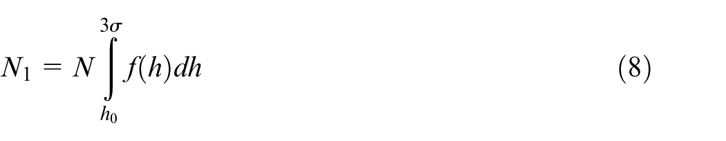
Researches and experiments show that the heights of abrasive protrusion are not the same.¹⁵ Therefore, only a part of grains will participate in the polishing process and this kind of grains are called the load-bearing grains which undertake the polishing force together.

The distribution of the heights of abrasive protrusion

Massive experiments and researches have shown that the maximum dimension $d_{\max}$ and average dimension $d_{m}$ of the abrasive grains are very close to the maximum and average heights of abrasive protrusion, respectively, as shown in Figure 1. Therefore, the distribution of the heights of abrasive protrusion is taken to be Gaussian distribution,¹⁶ that is

f (h) = \frac{1}{\sqrt{2 π} σ} e^{- {(h - u)}^{2} / 2 σ^{2}} | h | \leq 3 σ

(1)

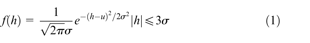
In the equation above, h stands for the height of abrasive protrusion, u is the mathematical expectation of h and $σ$ is the standard deviation which can be given by

σ = \frac{(d_{\max} - d_{m})}{3}

(2)

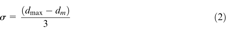
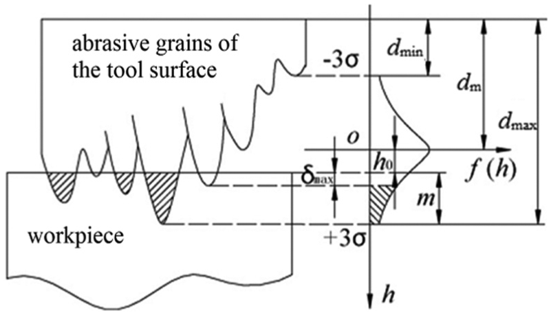
where $d_{\max}$ , $d_{m}$ and $σ$ for different grit designations are shown in Table 1.

Figure 1.

Schematic diagram of the height distribution of abrasive protrusion.

Table 1.

Values of $d_{m}$ , $d_{\max}$ and $σ$ for different grit designations.

M	d_m (μm)	d _max (μm)	σ (μm)
100	150	137.5	4.17
120	125	115.5	3.17
150	106	90.5	5.17
180	90	76.5	4.5
220	75	64	3.67
240	40	34	2

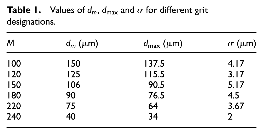
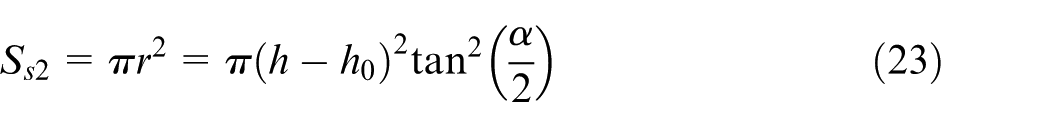
Figure 1 is a schematic diagram of the protrusion heights’ distribution on the polishing tool surface, and the origin point of the coordinate system is fixed on the horizontal position of $d_{m}$ . In Figure 1, $d_{\min}$ is the minimum dimension of the abrasive grains, the vertical distance between the origin point and the workpiece surface is $h_{0}$ , $δ_{\max}$ is the maximum overlap of elastic contact and m is the indentation depth of the highest grain.

The number of the load-bearing grains

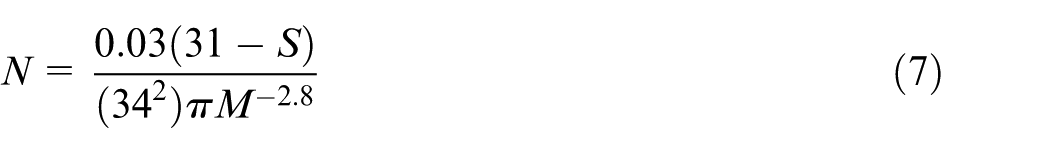
In this article, the structural number S and the grit designation M are taken as the two basic variables for abrasive characteristics. A polishing tool is composed of abrasive grains, bond and air vent. The structure number S stands for the volume ratio of the grains in the whole element volume. The relationship of S and volume ratio is obtained as follows²⁰

V_{g} = 2 (31 - S)

(3)

where V_g (%) is the grain ratio. For instance, V_g is 0.62 when S = 0 and 0.44 when S = 9.

The grit designation M is used to characterize the dimension d of the abrasive grains. The corresponding relationship of M and the dimension d can be calculated as follows²⁰

d_{m} = 68 M^{- 1.4}

(4)

d_{\max} = 15.2 M^{- 1}

(5)

Then the number of the abrasive grains per unit area N can be calculated as²¹

N = \frac{6 \times V_{g}}{π {d_{m}}^{2}}

(6)

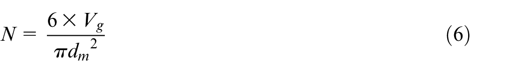
Equation (6) indicates that the structural number S and the grit designation M together determine the total number of the abrasive grains per unit area. From equations (3)–(6), the total number can be obtained as the following form

N = \frac{0.03 (31 - S)}{(34^{2}) π M^{- 2.8}}

(7)

Through the analysis in section “The distribution of the heights of abrasive protrusion,” it can be concluded that in the polishing process, not all the grains are involved in the polishing process. As shown in Figure 1, a grain would contact with the workpiece and support the polishing force only when the protrusion height is bigger than $h_{0}$ . Therefore, from equations (1) and (7), the number of load-bearing grains per unit area can be obtained in the following form

N_{1} = N \int_{h_{0}}^{3 σ} f (h) d h

(8)

The polishing force on a single abrasive grain

The polishing process is a complex material removal process involving rubbing, scratching, plowing and cutting between the workpiece and abrasive grains. It can be divided into two phases: the elastic deformation and plastic deformation according to the behavior of material deformation.¹⁵ The transition between the two phases depends on the cutting depth of the abrasive grains. In this section, the two phases are analyzed in detail, and the theory of contact mechanics and the force equilibrium are adopted to develop the relationship between the polishing force and the cutting depth.

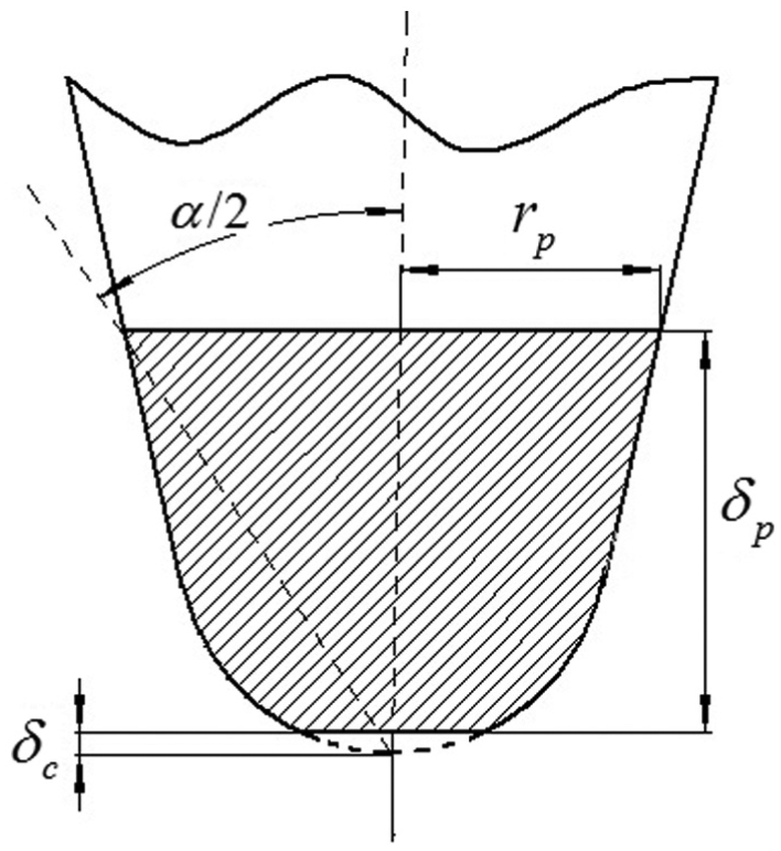
The transverse shape of the grooves produced by abrasive grains has been assumed to be triangular in most of the models developed so far.^15,16 In reality, a single abrasive grain typically has a lot of tiny cutting edges on its tip, which is similar to a multiple-point circular arc. The experiments conducted by Lal and Shaw²² with a single abrasive grain indicate that the grain tip could be better approximated by circular arc. Therefore, in this article, the shape of abrasive grains is assumed to be conic with spherical tip which means that the transverse shape is conic when the cutting depth is big and the transverse shape is spherical when the cutting depth is small.

Elastic deformation

According to the elastic mechanics theory, for a single abrasive grain, when a normal force $F_{0}$ is applied on the workpiece, as shown in Figure 2, then the following equations could be obtained²³

r = {(\frac{3 R F_{0}}{4 E^{*}})}^{1 / 3}

(9)

δ = {(\frac{9 F_{0}^{2}}{16 R E^{* 2}})}^{1 / 3}

(10)

p_{0} = \frac{1}{π} {(\frac{16 {E^{*}}^{2} F_{0}}{9 R^{2}})}^{1 / 3}

(11)

\frac{1}{E^{*}} = \frac{1 - ν_{3}^{2}}{E_{3}} + \frac{1 - ν_{2}^{2}}{E_{2}}

(12)

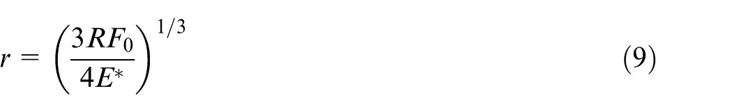
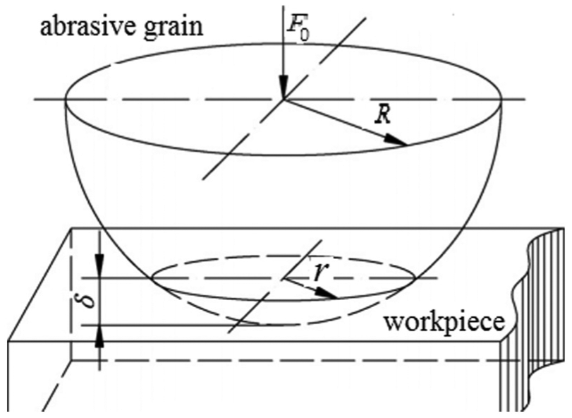
In these equations, R is the spherical radius of the abrasive grains’ tip; r is the radius of the circular contact area; $δ$ is the overlap of elastic contact; $p_{0}$ is the mean contact pressure; $E^{*}$ is the contact modulus of the abrasive grain and the workpiece; $E_{2}$ and $E_{3}$ are the Young’s modulus of the workpiece and the abrasive grain, respectively; $ν_{2}$ and $ν_{3}$ are the Poisson’s ratios of the workpiece and the abrasive grain, respectively.

Figure 2.

Schematic diagram of a single abrasive grain acted on the workpiece.

According to the elastic–plastic deformation theory, there will be plastic deformation on the workpiece surface when the mean contact pressure is bigger than H_B/3,^15,16 where $H_{B}$ is the Brinell hardness of the workpiece surface; conversely, there is only elastic deformation on the workpiece surface. From equations (10) and (11), the maximum overlap of elastic contact $δ_{\max}$ can be expressed as

δ_{\max} = \frac{π^{2} {R H}_{B}^{2}}{16 {E^{*}}^{2}}

(13)

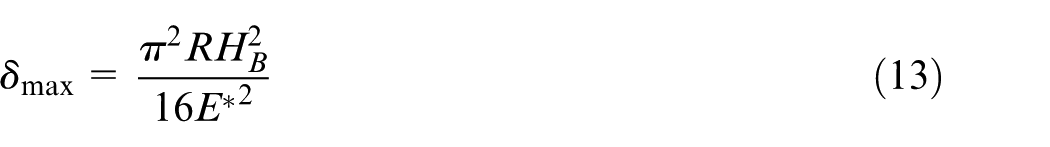
Therefore, when the height of abrasive protrusion belongs to $[h_{0}, h_{0} + δ_{\max}]$ , there is only elastic deformation on the workpiece surface, and the number of abrasive grains in this phase per unit area can be calculated as

N_{t} = N \int_{h_{0}}^{h_{0} + δ_{\max}} f (h) d h

(14)

From equation (10), solving for $F_{0}$ yields

F_{0} = \frac{4 E^{*} R^{1 / 2} {(h - h_{0})}^{3 / 2}}{3}

(15)

The force $F_{t}$ produced by the elastic deformation per unit area can be obtained from equations (14) and (15), and it is expressed as

\begin{matrix} F_{t} = N_{t} F_{0} \\ = \frac{4 N E^{*} \sqrt{R}}{3 σ \sqrt{2 π}} \int_{h_{0}}^{h_{0} + δ_{\max}} {(h - h_{0})}^{3 / 2} Δ d h \end{matrix}

(16)

where $Δ = e^{- h^{2} / 2 σ^{2}}$ .

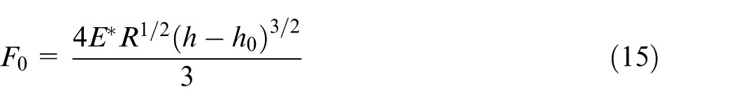
Plastic deformation

From the analysis above, it is known that there will be plastic deformation on the workpiece surface when the height of abrasive protrusion is bigger than $δ_{\max} + h_{0}$ .

As mentioned at the beginning of section “The polishing force on a single abrasive grain,” the transverse shape is different as the cutting depth varies. Therefore, the plastic deformation is divided into two phases in this part to make the analysis more conform to the reality.

Phase 1: the phase of spherical cutting

When the cutting depth is smaller than the spherical radius of the abrasive grain’s tip R, the process of spherical cutting takes place. In the actual polishing process, the plastic deformation is always accompanied by the presence of elastic deformation as shown in Figure 3. $δ_{c}$ is the depth of elastic deformation and the part in the area of the oblique lines is the transverse shape of the plastical cutting. According to the elastic–plastic deformation theory, $δ_{c}$ can be expressed as²⁴

δ_{c} = {(\frac{0.6 π H_{B}}{2 E^{*}})}^{2} R

(17)

Figure 3.

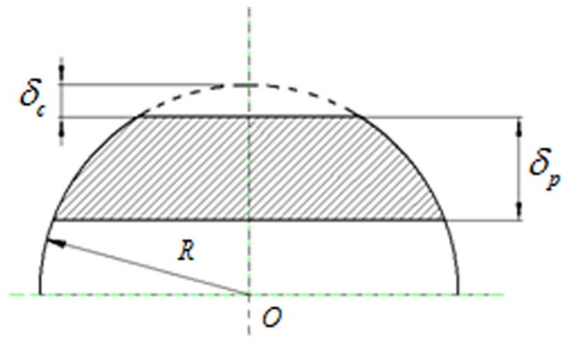
Schematic diagram of the spherical cutting of a single abrasive grain.

And the corresponding force caused by the elastic deformation can be calculated as²⁴

F_{c} = \frac{4}{3} E^{*} \sqrt{R} δ_{c}^{3 / 2}

(18)

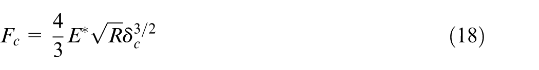
Here, if $δ_{p}$ is denoted as the cutting depth, then the corresponding force caused by the plastic deformation can be calculated as²⁰

F_{p} = 2 H_{B} π R δ_{p}

(19)

From equations (18) and (19), the total force on a single abrasive grain in the phase of spherical cutting is given by

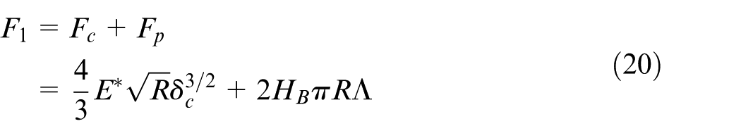
\begin{matrix} F_{1} = F_{c} + F_{p} \\ = \frac{4}{3} E^{*} \sqrt{R} δ_{c}^{3 / 2} + 2 H_{B} π R Λ \end{matrix}

(20)

where $Λ = h - h_{0} - δ_{c}$ .

The number of abrasive grains per unit area in this phase can be expressed as

N_{21} = N \int_{h_{0} + δ_{\max}}^{h_{0} + R} f (h) d h

(21)

From equations (20) and (21), the total force per unit area in the phase of spherical cutting can be written as

\begin{matrix} F_{s 1} = N_{21} F_{1} = \frac{4 \sqrt{R} δ_{c}^{3 / 2} N E^{*}}{3 σ \sqrt{2 π}} \int_{h_{0} + δ_{\max}}^{h_{0} + R} Δ d h \\ + \frac{2 H_{B} π R N}{\sqrt{2 π} σ} \int_{h_{0} + δ_{\max}}^{h_{0} + R} Δ Λ d h \end{matrix}

(22)

Phase 2: the phase of conic cutting

When the cutting depth is bigger than the spherical radius of the abrasive grain’s tip R, the process of conic cutting takes place and the cross section of the removed material is shown in Figure 4. In this phase, the elastic deformation will also occur. It is known from equation (17) that the elastic deformation is merely a function of R. Therefore, the depth and force caused by the elastic deformation are the same in the phase of spherical cutting and conic cutting.

Figure 4.

Schematic diagram of the conic cutting of a single abrasive grain.

In the phase of conic cutting, the pressure caused by the plastic deformation is always set to be $p_{1} = H_{B} / 2$ .^15,16 It is found that the shape of the contact area is circular, the radius r_p of which is equal to $(h - h_{0}) \tan (α / 2)$ , where $α$ is the apical angle of the cone. Therefore, the contact area can be expressed as

S_{s 2} = π r^{2} = π (h - h_{0})^{2} \tan^{2} (\frac{α}{2})

(23)

The number of abrasive grains per unit area in this phase can be calculated as

N_{22} = N \int_{h_{0} + R}^{3 σ} f (h) d h

(24)

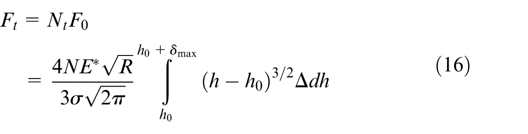
Thus, the total force per unit area caused by the plastic deformation in the phase of conic cutting is written as

\begin{matrix} F_{s 2} = N_{22} (F_{c} + S_{s 2} p_{1}) = \frac{4 \sqrt{R} δ_{c}^{3 / 2} N E *}{3 σ \sqrt{2 π}} \int_{h_{0} + R}^{3 σ} Δ d h \\ + \frac{H_{B} π N \tan^{2} (α / 2)}{2 \sqrt{2 π} σ} \int_{h_{0} + R}^{3 σ} Δ (h - h_{0})^{2} d h \end{matrix}

(25)

The model of the maximum cutting depth

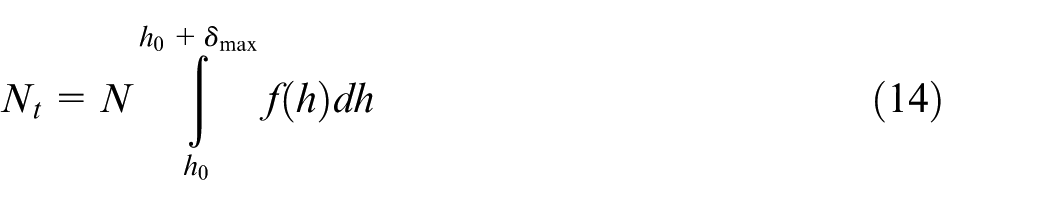
As analyzed above, the sum of the individual force on the load-bearing grains is equal to the normal polishing force. Based on the assumption, the relationship between the normal polishing force per unit area P (pressure) and the cutting depth of abrasive grains can be established. According to the value of the maximum cutting depth m, the following three cases are contained:

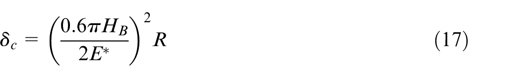
When $0 \leq m \leq δ_{\max}$ , there is only the elastic deformation, and the pressure is given by

P = F_{t}

(26)

When $δ_{\max} \leq m \leq R$ , the elastic deformation and the plastic deformation (spherical cutting) will occur simultaneously, and the pressure can be calculated as

P = F_{t} + F_{s 1}

(27)

When $R \leq m \leq 6 σ$ , the elastic deformation and the plastic deformation (spherical cutting and conic cutting) will occur simultaneously, and the pressure can be calculated as

P = F_{t} + F_{s 1} + F_{s 2}

(28)

In this article, the pressure distribution is assumed to accord with Hertz contact theory which is shown in Appendix 2. In case of a known pressure distribution, the maximum cutting depth of the abrasive grains could be obtained based on equations (26)–(28) which will be the input parameter of ANN.

Prediction model of surface roughness

ANN

ANN is currently one of the most widely used intelligent algorithms because of its characteristics of self-organizing, self-learning and self-adaption to nonlinear system. It has been used in diverse applications in control, robotics, pattern recognition, forecasting, power systems, manufacturing, optimization, signal processing and so on. There are various kinds of ANN models among which BP network is applied most broadly.¹³ BP neural network, which is a kind of multilayer feedforward network based on the error BP algorithm, consists of two processes: forward-propagation of the information and BP of the error. Based on the difference between the actual output and the desired output, the steepest descent algorithm is used to constantly adjust the weights and thresholds of the network until the sum of the squared error (SSE) is acceptable. BP neural network is good at solving nonlinearity problem with the characters of high operability, self-organizing configuration and stable working condition, so it is chosen to model surface roughness in this article.

The prediction model based on BP network

The BP network is composed of a set of neurons grouped in layers. Usually, three types of layers are used: input layer, hidden layer and output layer. The BP neural network architecture used in this article is shown in Figure 5. The basic steps of BP prediction model can be summarized as follows.

Figure 5.

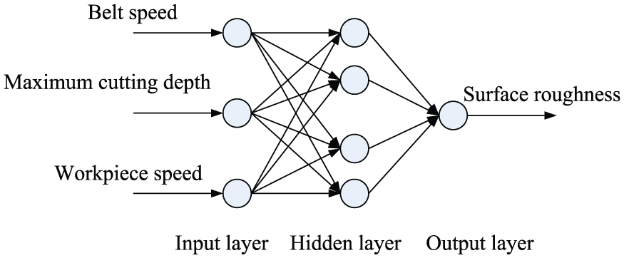
The architecture of BP neural network.

Parameters’ definition and data normalization

In this article, the input parameters can be divided into two types. The first type is the microscopic parameter, namely, the maximum cut depth of abrasive grains which can be solved by the model in section “The model of cutting depth.” The second type contains two macroscopic parameters, including belt speed and the feed rate of the workpiece which are set by the process. The output of the BP network is the value of surface roughness Ra.

Then, for stability reasons, it is necessary to normalize the values of the input and output data to a specific range, which is commonly between 0 and 1. Here, the arithmetic mean method is adopted and the normalized values can be calculated by

X_{c} (k) = \frac{X_{c j} (k) - X_{c \min} (k)}{X_{c \max} (k) - X_{c \min} (k)}

(29)

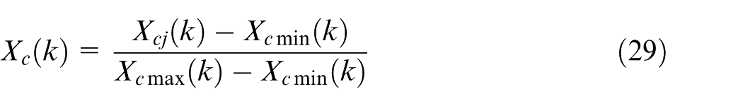
where $X_{c j}$ is the sample value before normalization; $X_{c \max}$ and $X_{c \min}$ are the maximum and minimum values of sample data, respectively.

Network initialization

In this article, the hidden layer consists of 11 neurons. The activation function of the hidden layers is the Tan-sigmoid transfer function, and linear transfer function is used for the output layer. Levenberg–Marquardt (LM) algorithm is selected for training the ANN. Mean square error (MSE) is used to detect the deviation between the output data of the network.

Network training and testing

In this part, the sample data are divided into two groups, namely, the training samples and the testing samples. During the training, the input data are presented to the network and the output data of the network are compared with the desired output. The training stops when MSE is less than the goal value (0.001). Then the trained neural network is tested using testing samples, and the prediction results are used to verify the model in this article.

The flow chart of the prediction model

The flow chart of the roughness prediction model is shown in Figure 6. The process can be divided into two parts: the calculation of the maximum abrasive cutting depth and roughness prediction model based on BP neural network. The maximum abrasive cutting depth can be calculated by the model in section “The model of cutting depth” and then it together with the other two parameters, namely, the feed rate of workpiece and belt speed, are used as the input parameters to train and test the prediction model.

Figure 6.

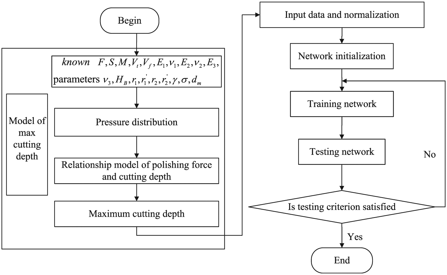
The flow chart of the surface roughness prediction model.

Experimental results and discussion

To evaluate the proposed model in this article, the predicted results are compared with the experiment data reported in the dissertation by Ding.²⁵ The experimental platform is a cylindrical computer numerical control (CNC) polishing machine, the workpiece is an A356 aluminum alloy wheel and the polishing tool is a belt wheel as shown in Figure 7. The other parameters are shown in Table 2, and the meaning of the parameters can be seen in Appendix 1.

Figure 7.

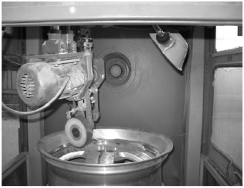
Schematic diagram of the belt polishing.²⁵

Table 2.

The adopted process parameters.²⁵

Items	Conditions
Grains	M = 240, E₃ = 400 GPa, ν₃ = 0.3, α = 90°, R = 2.792 μm
Tool	E ₁ = 25 MPa, ν₁ = 0.10, r₁ = 50 mm, $r'_{1} = \infty$ , S = 0
Workpiece	E ₂ = 72.4 GPa, ν₂ = 0.33, r₂ = 20 mm, $r'_{2} = 100 mm$ , H_B = 686 MPa
Other parameters	γ = 0°, F = 5, 10, 15, 20, 25, 30 N, V_f = 0.05, 0.1, 0.16, 0.22, 0.27 m/min, V_t = 7.5, 8.5, 9.5, 10.5, 11.5 m/min

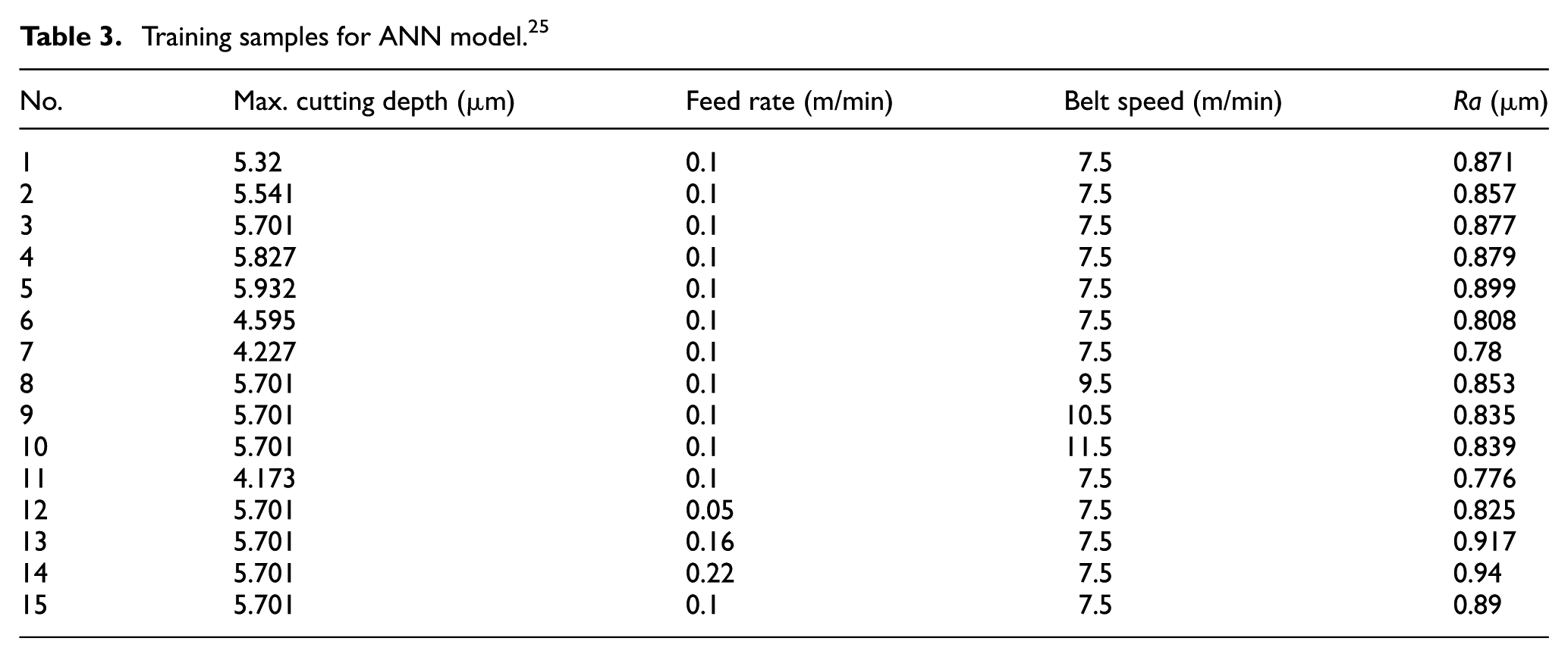
In this article, 20 samples are selected from the dissertation²⁵ among which 15 groups are selected as the training samples and the remaining 5 groups as the testing samples, as shown in Tables 3 and 4, respectively. The parameters of belt speed and feed rate of the workpiece are also given by the dissertation²⁵ and the maximum cutting depth can be obtained using the model in section “The model of cutting depth.”

Table 3.

Training samples for ANN model.²⁵

No.	Max. cutting depth (μm)	Feed rate (m/min)	Belt speed (m/min)	Ra (μm)
1	5.32	0.1	7.5	0.871
2	5.541	0.1	7.5	0.857
3	5.701	0.1	7.5	0.877
4	5.827	0.1	7.5	0.879
5	5.932	0.1	7.5	0.899
6	4.595	0.1	7.5	0.808
7	4.227	0.1	7.5	0.78
8	5.701	0.1	9.5	0.853
9	5.701	0.1	10.5	0.835
10	5.701	0.1	11.5	0.839
11	4.173	0.1	7.5	0.776
12	5.701	0.05	7.5	0.825
13	5.701	0.16	7.5	0.917
14	5.701	0.22	7.5	0.94
15	5.701	0.1	7.5	0.89

Table 4.

Testing samples for ANN model and prediction results.²⁵

No.	Max cutting depth (μm)	Feed rate (m/min)	Belt speed (m/min)	Ra (μm)
No.	Max cutting depth (μm)	Feed rate (m/min)	Belt speed (m/min)	Experimental results²⁵	Results in dissertation²⁵	Results in this article
1	5.897	0.1	7.5	0.89	0.878	0.889
2	4.788	0.1	7.5	0.824	0.83	0.842
3	5.701	0.27	7.5	0.98	0.962	0.961
4	5.701	0.1	8.5	0.851	0.86	0.839
5	5.701	0.1	7.5	0.863	0.872	0.86
Average relative error					1.2%	1.19%

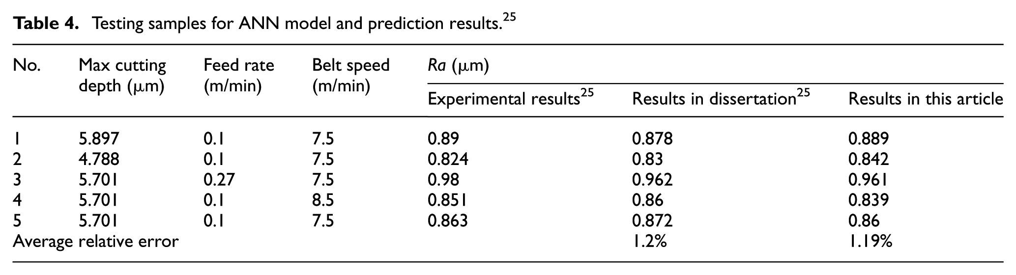
Figure 8 shows the training epoch versus MSE from which it can be found that the training step stops at 24th epoch when MSE is less than the goal value (0.001) during training. While in the dissertation,²⁵ the number of epoch is about 60. Therefore, the BP neural network in this article has a faster convergence rate because compared with the model in the dissertation,²⁵ the number of input parameters and testing samples in this article is smaller. The testing results are listed in Table 4, and the two prediction methods show a good fitting accuracy. It can be seen that the average prediction error of the dissertation²⁵ is 1.2%, and it is 1.19% in this article which shows no obvious difference and proves that both of them have a high degree of accuracy.

Figure 8.

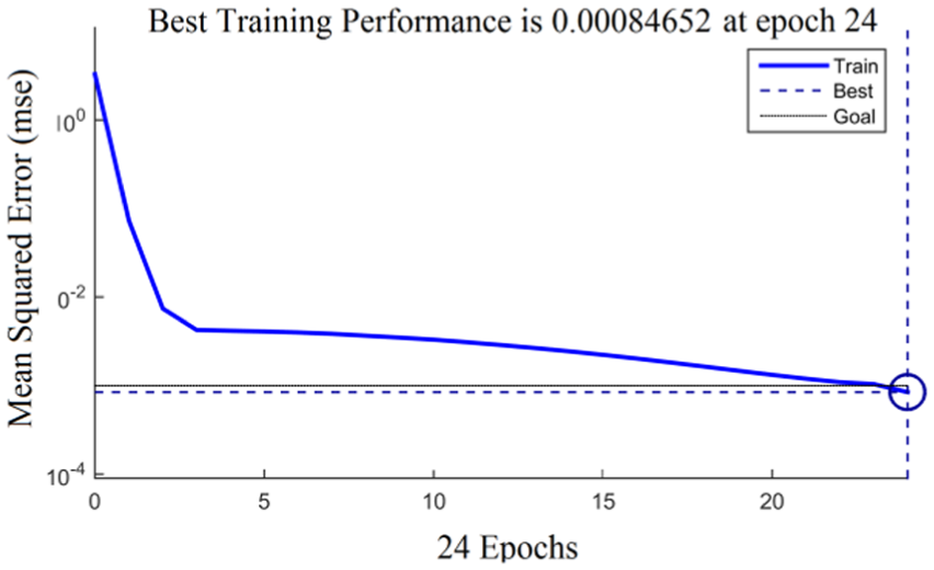
The training epoch versus MSE.

However, there is a fact that the number of training samples in the dissertation²⁵ is 193 while it is 15 in this article. The results above show that on the premise that the prediction accuracy can be met, the prediction model in this article has a faster convergence rate and requires fewer experimental data which will save the cost and time of the experiments. This is because compared with the polishing force, the abrasive cutting depth can reflect the surface roughness more comprehensively. Therefore, the model can reflect the formation mechanism and the value of surface roughness more comprehensively and precisely by taking the maximum cutting depth into consideration.

Conclusion

In this article, a predictive model of surface roughness based on ANN in belt polishing is presented. Comparison between the prediction and experimental results shows a good consistency which verifies the theoretical model. The work in this article is concluded as follows:

From the perspective of the grains, the grit designation and structural number are used as the two basic variables for abrasive characteristics, and it is assumed that the shape of an abrasive grain is conic with spherical tip, which fully takes into account the characteristics of the abrasive grains.

Different stages of the deformations of the workpiece during the polishing process are decomposed in detail in the model. With the consideration that the plastic deformation is accompanied by the presence of elastic deformation, the model of the cutting depth in this article is more realistic.

Based on the work above, and by the use of the elastic contact theory and the plastic contact theory, the model of the cutting depth for the polishing process is developed.

The maximum cutting depth together with the other parameters is used as the input parameter and then the ANN prediction model for surface roughness is presented finally.

Compared with the polishing force, the abrasive cutting depth contains more parameters that have effect on surface roughness and reflects the nature of the roughness more comprehensively. On the premise that the prediction accuracy can be met, the prediction model in this article has a faster convergence rate and requires fewer experimental data which will save the cost and time of the experiments. In addition, the model can be applied to different situations such as polishing under different workpieces and polishing wheels, so it has a wider range of applications with better application prospects.

Footnotes

Appendix 1

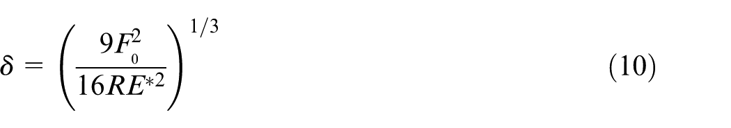
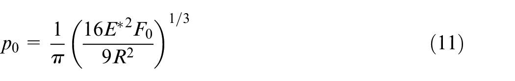
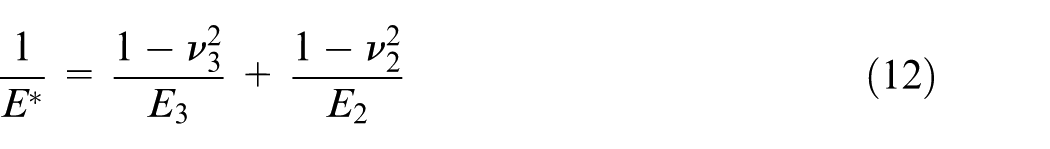
Appendix 2

The pressure distribution equation is as follows

(30)

p (x, y) = p_{0} \sqrt{1 - \frac{x^{2}}{a^{2}} - \frac{y^{2}}{b^{2}}}

where $p_{0}$ is the maximum contact pressure located at the center of the contact ellipse. $p_{0}$ , a and b can be calculated as follows

(31)

p_{0} = \frac{3 F}{2 π a b}

(32)

a = {[\frac{3 k_{2}^{2} ε (k_{1}) F}{π E_{1}^{*} (A + B)}]}^{1 / 3}

(33)

b = {[\frac{3 ε (k_{1}) F}{π k_{2} E_{1}^{*} (A + B)}]}^{1 / 3}

where F is the applied force between the tool and the workpiece surface, $E_{1}^{*}$ is the contact modulus of the workpiece and the tool which can be given by $(1 / E_{1}^{*}) = ((1 - ν_{1}^{2}) / (E_{1})) + ((1 - ν_{2}^{2}) / (E_{2}))$ and $E_{1}$ and $ν_{1}$ refer to Young’s modulus and Poisson’s ratio of the polishing tool, respectively. The other parameters can be calculated as follows

(34)

k_{1} = \frac{a}{b} \approx 1.0339 {(\frac{B}{A})}^{0.636}

(35)

ε (k_{1}) = 1.0003 + 0.5968 (\frac{A}{B})

(36)

A + B = \frac{1}{2} (\frac{1}{r_{1}} + \frac{1}{{r'}_{1}} + \frac{1}{r_{2}} + \frac{1}{{r'}_{2}})

(37)

B - A = \frac{1}{2} \sqrt{{(\frac{{r'}_{1} - r_{1}}{r_{1} {r'}_{1}})}^{2} + {(\frac{{r'}_{2} - r_{2}}{r_{2} {r'}_{2}})}^{2} + 2 (\frac{{r'}_{1} - r_{1}}{r_{1} {r'}_{1}}) (\frac{{r'}_{2} - r_{2}}{r_{2} {r'}_{2}}) \cos 2 γ}

where $r_{1}$ and $r'_{1}$ are the principal radii of curvature of the polishing tool at the contacting point, $r_{2}$ and $r'_{2}$ are the principal radii of curvature of the workpiece at the contacting point and $γ$ is the included angle between the directions of principle curvature of the workpiece and the tool at the contacting point.

Acknowledgements

The experimental data in the last part of this article are cited from the group of Changlin Wu of Huazhong University of Science and Technology. And the authors are grateful for the permissions.

Declaration of conflicting interests

The author(s) declared no potential conflicts of interest with respect to the research, authorship and/or publication of this article.

Funding

The author(s) disclosed receipt of the following financial support for the research, authorship, and/or publication of this article: This study was supported by the Fundamental Research Funds for the Central Universities (Grant no. 3102015JCS05012).

References

Pan

Wang

Jiang

. A novel method for aspheric polishing based on abrasive trajectories analysis on contact region. Proc IMechE, Part B: J Engineering Manufacture 2015; 229(2): 275–285.

Sun

Feng

. Automatic robotic polishing on titanium alloy parts with compliant force/position control. Proc IMechE, Part B: J Engineering Manufacture 2015; 229(7): 1180–1192.

Tsai

Wang

Tsai

. Investigation of increased removal rate during polishing of single-crystal silicon carbide. Int J Adv Manuf Techn 2015; 80(9–12): 1511–1520.

Lee

. Prediction of surface roughness in magnetic abrasive finishing using acoustic emission and force sensor data fusion. Proc IMechE, Part B: J Engineering Manufacture 2011; 225(6): 853–865.

Ghadikolaei

Vahdati

. Experimental study on the effect of finishing parameters on surface roughness in magneto-rheological abrasive flow finishing process. Proc IMechE, Part B: J Engineering Manufacture 2014; 229(9): 1517–1524.

Kant

Sangwan

. Predictive modelling and optimization of machining parameters to minimize surface roughness using artificial neural network coupled with genetic algorithm. Procedia CIRP 2015; 31: 453–458.

Wei

Yang

. Investigation of factors influencing microscopic interactions between the diamond indenter and material surfaces in nano-indentation. Appl Surf Sci 2015; 355: 761–765.

Belkhir

Aliouane

Bouzid

. Correlation between contact surface and friction during the optical glass polishing. Appl Surf Sci 2014; 288: 208–214.

Ahn

Shen

Kim

. Development of a sensor information integrated expert system for optimizing die polishing. Robot Cim: Int Manuf 2001; 17(4): 269–276.

10.

Márquez

Pérez

Rıos

. Process modeling for robotic polishing. J Mater Process Tech 2005; 159(1): 69–82.

11.

Wang

. Research on polishing process of a special polishing machine tool. Mach Sci Technol 2009; 13(1): 106–121.

12.

Sangwan

Saxena

Kant

. Optimization of machining parameters to minimize surface roughness using integrated ANN-GA approach. Procedia CIRP 2015; 29: 305–310.

13.

Wang

Zhao

. Process optimization of the serial-parallel hybrid polishing machine tool based on artificial neural network and genetic algorithm. J Intell Manuf 2012; 23(3): 365–374.

14.

Durmuş

Özkaya

Meri

. The use of neural networks for the prediction of wear loss and surface roughness of AA 6351 aluminium alloy. Mater Design 2006; 27(2): 156–159.

15.

Ding

Chen

. Research on modeling method of material removal depth in CNC mechanical polishing for aluminum alloy wheel. China Mech Eng 2009; 20(21): 2558–2562.

16.

Wang

. Modeling and analysis of the material removal depth for stone polishing. J Mater Process Tech 2009; 209(5): 2453–2463.

17.

Hecker

Liang

. Predictive modeling of surface roughness in grinding. Int J Mach Tool Manu 2003; 43(8): 755–761.

18.

Ren

Cabaravdic

Zhang

. A local process model for simulation of robotic belt grinding. Int J Mach Tool Manu 2007; 47(6): 962–970.

19.

Chang

Farris

Chandrasekar

. Contact mechanics of superfinishing. J Tribol 2000; 122(2): 388–393.

20.

Zhou

. Modeling surface roughness in the stone polishing process. Int J Mach Tool Manu 2005; 45(4): 365–372.

21.

Doman

Warkentin

Bauer

. A survey of recent grinding wheel topography models. Int J Mach Tool Manu 2006; 46(3): 343–352.

22.

Lal

Shaw

. The role of grain tip radius in fine grinding. J Eng Ind 1975; 97(3): 1119–1125.

23.

Xie

Williams

. The prediction of friction and wear when a soft surface slides against a harder rough surface. Wear 1996; 196(1): 21–34.

24.

Chang

Etsion

Bogy

. An elastic-plastic model for the contact of rough surfaces. J Tribol 1987; 109(2): 257–263.

25.

Ding

. Basic research on process optimization for CNC mechanical polishing aluminum alloy wheel. PhD Thesis, Huazhong University of Science and Technology, China, 2010.

Modeling and prediction of surface roughness in belt polishing based on artificial neural network

Abstract

Keywords

Introduction

The model of cutting depth

The number of the load-bearing grains

The distribution of the heights of abrasive protrusion

The number of the load-bearing grains

The polishing force on a single abrasive grain

Elastic deformation

Plastic deformation

Phase 1: the phase of spherical cutting

Phase 2: the phase of conic cutting

The model of the maximum cutting depth

Prediction model of surface roughness

ANN

The prediction model based on BP network

Parameters’ definition and data normalization

Network initialization

Network training and testing

The flow chart of the prediction model

Experimental results and discussion

Conclusion

Footnotes

Appendix 1

Appendix 2

Acknowledgements

Declaration of conflicting interests

Funding

References