Sage Journals: Discover world-class research

Abstract

Nickel-based alloys are a class of hard-to-machine materials that exhibit a unique combination of high strength at high temperature. While they are widely used in industry, the high tool wear rate of these materials makes machining them a challenging task. Furthermore, machining tolerances, residual stresses, and tool runout impose uncertainty in tracking tool wear. In this work, the current view on tracking progressive tool wear is shifted from deterministic domains into the stochastic domain to study the probability distribution of the tool wear during the process. To do so, Bayesian-based estimation was used for accurate model inference and the result was fed into the Kalman filter for tracking tool wear in end-milling Rene-108 Ni-based alloy. To improve the accuracy, a direct laser measuring system for capturing tool length change was fused with the indirect power measurement. The results show a significant improvement in accuracy over the indirect method, with less than 8 µm root mean square error. This measuring strategy improved the accuracy, while preserving the automated platform for monitoring the tool’s health.

Keywords

Tool wear Bayesian Kalman filter milling nickel-based alloy monitoring

Introduction

Automation of tool condition monitoring (TCM) is gaining more attention in manufacturing processes in recent times. A total of 20% of machining downtime is reported to be due to tool wear,¹ which causes surface deterioration and can be detrimental to machine health. Tool wear also limits the productivity rate, which has direct influence on profitability. With advances in developing new higher-performing materials in the power generation and advanced engines’ industries that are far more detrimental to cutting tools in the manufacturing process, the need for monitoring the state of the tool is becoming more important.

Tool wear monitoring can be done in a direct or indirect manner. Direct methods of tool wear measurement require direct access to the process. The process should be stopped, and the tool is evaluated using visual inspection or measurement with a pre-installed device. Because of direct access to the tool wear, these methods are more accurate for tool wear monitoring, but not very practical in automated manufacturing systems due to the tedious nature of the required work. In addition, when the whole process is stopped, machining downtime is increased and the rate of productivity is decreased. Recently, a non-intrusive digital image processing using machine vision has been utilized for automated monitoring of tool wear or workpiece surface texture analysis.^2,3 The existence of chips, dirt, or lubricating fluid in the machining environment and extra sensitivity to lighting condition are some of the major challenges for direct image processing strategies to be accepted in industrial machine shops.⁴ In an early work by Sortino,⁵ he used a statistical bi-dimensional high-pass filter for processing camera images of the cutting tool and detecting borderlines of worn land. Sortino showed that using the mean and standard deviation of each pixel and its corresponding neighboring pixels provides enough information for detecting worn land of the tool surface. In a recent effort by Shahabi and Ratnam,⁶ a charge coupled device (CCD) camera was used with Wiener filtering for image noise suppression in various cutting conditions; it was shown that the effect of environmental factors can be significantly reduced using this method. Kuttolamadom et al.⁷ used a three-dimensional (3D) image of a carbide insert with complex geometry, developed under optical surface profiler in milling Ti6Al4V alloy. The 3D image of the worn insert was later used to find the correlation between volumetric tool wear rate and material removal rate in milling operation.⁸

An alternative for direct methods of studying tool wear is indirect methods, in which directly observed external signals such as acoustic emission, machining forces, spindle power consumption, and vibration are related to the tool wear state. The advantage of indirect methods over direct methods is that there is no need to interrupt the process, so they can be incorporated in automated machining processes without the loss of productivity. The main disadvantage is the existence of noise in signals, which induces uncertainty, and requires advanced signal processing for extracting the relevant features of the signal to relate them to the tool wear.

Since 1907 when Taylor proposed his famous tool life model,⁹ several studies were conducted to understand the nucleation and dynamic evolution of tool wear in cutting processes. Several empirical or analytical models were proposed by researchers; however, the variability in materials, tooling geometry, coating, and cutting conditions in addition to lack of current knowledge in understating the wear dynamics have made establishing a general model impossible. All these factors make in-process tool wear tracking a challenging task. Understanding all underlying effects and interactions in the machining operation might be impossible, but these can be treated as sources of uncertainty. The uncertainties should then be quantified to improve the decision-making strategy for replacing the worn-out tool with a sharp one. Therefore, tool wear should be assumed as a probabilistic variable and the focus of indirect estimation algorithms should be shifted from tracking the actual flank wear to tracking its probability distribution.

In general, the indirect estimation strategies of monitoring tool wear can be divided into deterministic-based or probabilistic-based methods. While the deterministic methods such as neural network^10,11 and support vector machine¹² have been widely explored in the context of TCM, the probabilistic algorithms based on Bayes theorem are gaining more attention recently. The robustness, low computational cost, and ability to provide decision probability are some of the advantages of these algorithms over deterministic ones. The probabilistic-based algorithms can be used for model parameter calibration or state tracking purposes. One of the early works in model parameter calibration was stochastic estimation based on a mesh grid method for identifying unknown parameters in the orthogonal Merchant model.¹³ The identified parameters were fed into the model for predicting cutting force and its uncertainty, and the model was experimentally validated by turning AISI-1045 steel. In another work, the mesh grid method and Markov chain Monte Carlo (MCMC) were used for Bayesian parameter inference on Taylor tool life and extended Taylor life in milling of AISI-4137 steel;^14,15 here, it was shown that using a Bayesian method fewer experiments were required for parameter inference.

Besides parameter calibration, online tracking or classification strategies such as Bayesian network, hidden Markov models (HMMs), and Kalman/particle filters are examples of indirect probabilistic estimation strategies. Bayesian networks are classified as probabilistic graphical models for representing causal relation between causes and effects. Therefore, they are capable of diagnosing system’s root causes of variation. The Bayesian network has been used by Dey and Stori¹⁶ for identifying sources of variability in workpiece dimensional tolerances and tool wear in sequential machining processes with different sensors. The naive Bayes classifier as a subcategory of Bayesian networks has been used by Karandikar et al.¹⁷ for detecting tool wear state in both discrete and continuous scenarios in end-milling AISI-1018; low computational time and the ability for fusing information from multiple sensors were concluded as the advantages of naive Bayes algorithm. The ability of naive Bayes in fusing sensory signals for fault detection was also investigated by Mehta et al.¹⁸ for early detection of computer numerical control (CNC) spindle failure using temperature and ultrasonic sensors. Contrary to the Bayesian network which does not capture the temporal behavior of sensor signal, dynamic Bayesian networks, also known as HMMs, were introduced first in the speech recognition community¹⁹ and later found their way to different manufacturing operations such as micro-milling and turning.^20,21 In a study carried out by Scheffer et al., the performance of the HMM and neural network for tool wear classification was evaluated. It was shown that the ease of training HMM with the Baum–Welch algorithm is the major advantage of the HMM over a neural network.²² However, the drawback is that the HMM only works for classification purposes and cannot be used for continuous tracking of tool wear. For tracking a continuous state of a system, stochastic-based filters such as Kalman filter and particle filter were proposed. In these methods, the probability distribution of a system’s state or parameter is updated when the sensor measurement becomes available. The Kalman filter was used for estimating the tool wear in down-milling of a $γ'$ -strengthened alloy with a mechanical touch probe as the measurement device; it was shown that it performs better than the deterministic approach.²³ The performance comparison of the particle filter and the Kalman filter in wear probability characterization in both milling and turning was investigated by Akhavan Niaki et al.,^24,25 and it was shown that using the random sampling strategy of the particle filter, a more informative prior distribution function can be generated for online inference. Furthermore, the applicability of the particle filter with a continuous resampling strategy for joint state and time-varying parameter estimation was investigated by Wang and Gao^26,27 in predicting tool wear growth and engine performance tracking and was further validated with the experimental results.

Nickel-based alloys are among a class of hard-to-machine materials, with exceptional high strength and corrosion resistivity. However, machining cost plays an important role in introducing them to designs because of their strength and excessive temperature rise at the cutting zone due to their low conductivity. Because of the potential damage that tool failure may cause for the high-cost Ni-based workpiece, having an estimation of tool wear or other important parameters while machining these materials is of great importance. Reviewing the state-of-art articles published recently shows that several micro-scale level studies have been undertaken for understanding the dominant wear failure mechanisms in Ni-based alloys and the effect of machining parameters such as tool geometry and coating or lubrication on the tool wear.^28,29 However, online monitoring of the tool wear has not been addressed yet in depth except in a few articles.

This study aims at using a probabilistic-based method for online tracking of the tool wear in end-milling Rene-108 Ni-based alloy. To improve the performance, this article examines the applicability of using a laser system as direct measuring strategy with no human interruption and fuses its output with an indirect measuring method using the spindle power signal. The mathematical background of probabilistic tools will be discussed in section “Mathematical background” followed by proper model for power and laser measurement in section “Measurement models.” In section “Experimental setup, “machining setup will be explained and dominant wear failure modes will be identified. In sections “Random-walk Metropolis method for inference on cutting power model” and “Stochastic modeling of tool flank wear,” random-walk Metropolis algorithm will be used for calibrating parameters of power model, and discrete state space model for the Kalman filter is explained. The results and conclusions are then discussed in sections “Results and discussion” and “Conclusion,” respectively.

Mathematical background

Bayesian inference is being used to address the uncertainties of a system, model, or parameter in terms of probabilistic functions. Contrary to Frequentist inference where an event is considered deterministic with a single true value bounded by a confidence interval representing inaccuracy in measurement or model, in the Bayesian inference a true value does not exist. Instead, the event is considered as a random variable with certain probability distribution function and its uncertainty is described by a credible interval. The Bayesian inference can be done in two fashions: offline or online. In the offline inference, batch of experiments should be completed before making an inference to build up a likelihood probability function $p (Y | X)$ , where Y represents the measurements and X represents the unknown variables. Then the initial knowledge known as a prior belief of X, which is based on previous measurements or knowledge, is mixed with the likelihood probability to complete the inference and to produce a posterior probability of parameters X.

Unlike the Frequentist analysis which states performing enough measurements is adequate to define a system, in the Bayesian analysis the previous knowledge (p(X)) is combined with the measurements as shown in equation (1). Therefore, the Bayesian inference becomes distinguishable where limited measurements are available or running experiments are costly. In cases where a closed-form solution for the posterior probability is not available, it is described by producing enough samples from its distribution. MCMC methods such as random-walk Metropolis algorithm have an extensive use for this purpose

p (X | Y) \propto p (Y | X) p (X)

(1)

In the random-walk Metropolis algorithm described in Figure 1, a proposal density (usually a Gaussian distribution) close to the posterior distribution is chosen to draw samples from. The ratio of the probability of drawn samples to the probability of the previously chosen samples determines whether the samples should be accepted or rejected. By proper selection of the proposal density and drawing enough samples, the posterior distribution of X; $p (X | Y)$ can be identified.

Figure 1.

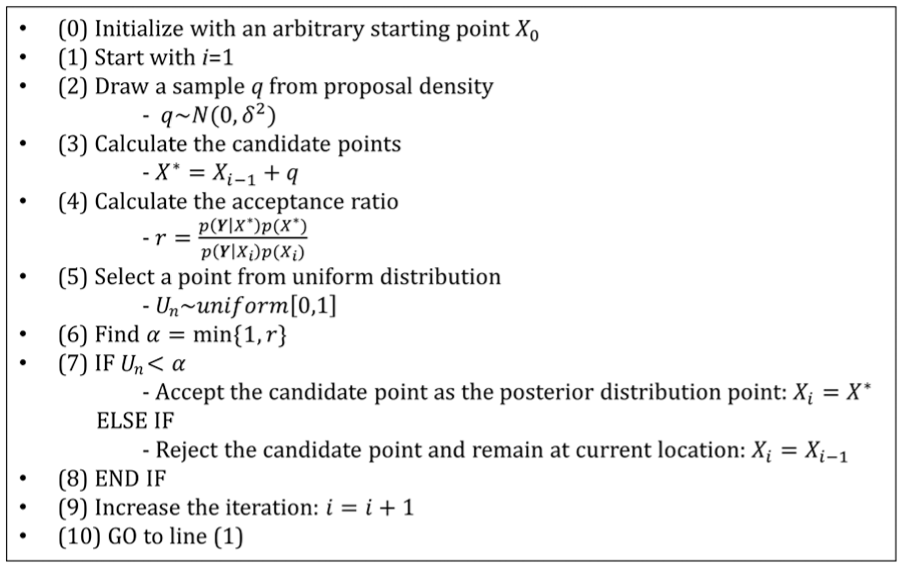
Pseudo code for random-walk Metropolis algorithm with normal proposal density function.³⁰

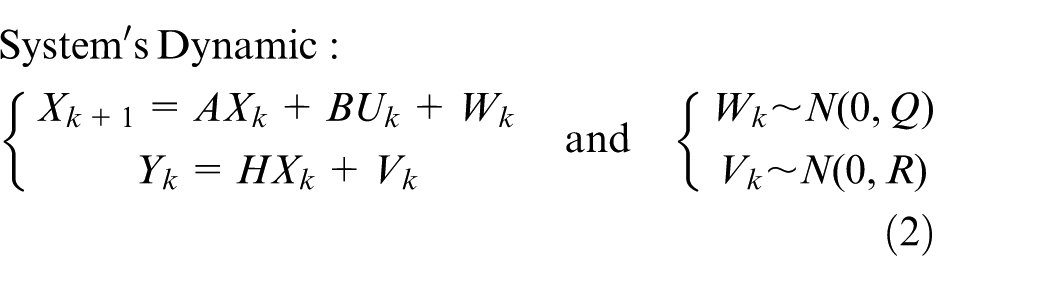
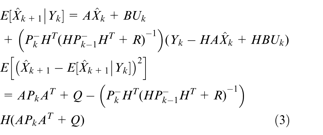
The offline Bayesian inference suits well to calibrate model parameters. However, to be able to describe the temporal behavior of a system, another approach should be taken. Assuming a dynamic system described in equation (2), and assuming a Gaussian probability function for unknown states (X), Rudolf Kalman found a closed-form solution to recursively update the mean and covariance of X over time. At each iteration k, the estimate of the mean and covariance of states will be updated based on the previous update ${\hat{X}}_{k}$ and P_k and later will be adjusted when the measurement Y_k becomes available. This is described in equation (3). Note that the state noise (W_k) and measurement noise (V_k) are characterized as Gaussian distributions with zero mean and covariance Q and R, respectively. Offline inference can be done to calibrate the model parameters and then the model can be used in the Kalman filter framework to make an online estimation of the system’s states. This is summarized in Figure 2

\begin{array}{l} {System}^{'} s Dynamic : \\ {\begin{matrix} X_{k + 1} = A X_{k} + B U_{k} + W_{k} \\ Y_{k} = H X_{k} + V_{k} \end{matrix} and {\begin{matrix} W_{k} ~ N (0, Q) \\ V_{k} ~ N (0, R) \end{matrix} \end{array}

(2)

At each iteration ↓

\begin{matrix} E [{\hat{X}}_{k + 1} | Y_{k}] = A {\hat{X}}_{k} + B U_{k} \\ + (P_{k}^{-} H^{T} {({HP}_{k - 1}^{-} H^{T} + R)}^{- 1}) (Y_{k} - HA {\hat{X}}_{k} + HB U_{k}) \\ E [{({\hat{X}}_{k + 1} - E [{\hat{X}}_{k + 1} | Y_{k}])}^{2}] \\ = A P_{k} A^{T} + Q - (P_{k}^{-} H^{T} {({HP}_{k - 1}^{-} H^{T} + R)}^{- 1}) \\ H (A P_{k} A^{T} + Q) \end{matrix}

(3)

Figure 2.

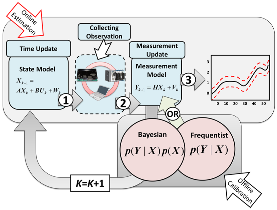
The Kalman filter diagram where the Bayesian-based or Frequentist-based models can be fed to as the measurement model.

Measurement models

Mechanistic tool wear model

Hall-effect sensors for measuring spindle current have the advantage of ease of installation and low cost. Therefore, these sensors were used to measure spindle power consumption shown as Y_k in equation (2). A mechanistic model already proposed by Shao et al.³¹ was chosen and is shown in equation (4), where P denotes the spindle power, N is the spindle speed (r/min), f is the feed, Vb is the tool flank wear, and K_i are unknown model parameters. These parameters should be determined for each specific tool–workpiece combination before using the model. It is also worth mentioning that in equation (4), power is linearly dependent on the tool wear when the cutting condition is constant

Pow = K_{1} N f^{K_{2}} + K_{3} NVb

(4)

Tool length change model

As the cutting tool wears out during the process, the length of the insert gradually decreases until catastrophic failure occurs. Therefore, direct measurement of the change in the length of the insert before and after the cutting process makes tool wear estimation possible. Mechanical touch probes have already been used to measure tool length change.²³ However, the process is time-consuming since it involves multiple repetitions to eliminate the measurement error. The application of laser in assisting the cutting process and reducing tool wear rate by thermal softening of metal has been shown previously in machining operations.^32,33 However, a laser measuring system can also be used as an alternative method to be implemented for precise and accurate measurement of the tool length and detecting tool breakage. Repeatability, quick measurement, and the ability to measure the length of rotating and non-rotating tools are some of the advantages of laser measurement systems over mechanical touch probes. Mechanical touch probes are prone to mechanical damage due to the direct contact of the tool to the probe, but the laser-based measuring system shown in Figure 3 makes non-contact measurement possible and eliminates the possibility of any damage to the tool or measurement device. However, high cost of implementation is a drawback of such systems.

Figure 3.

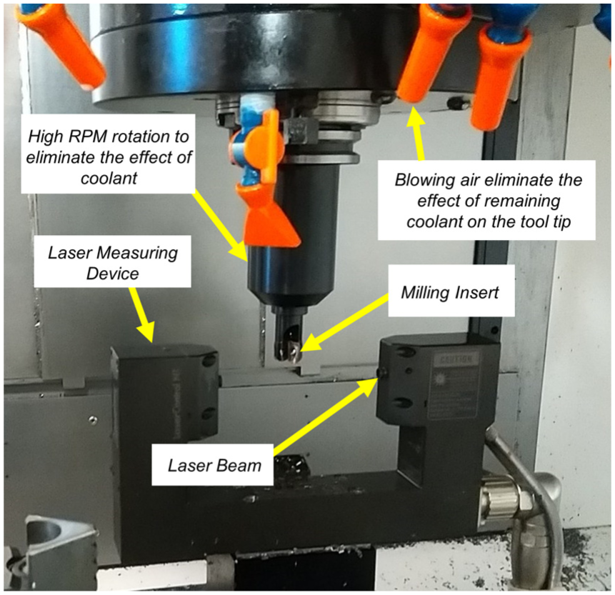
Laser measuring device.

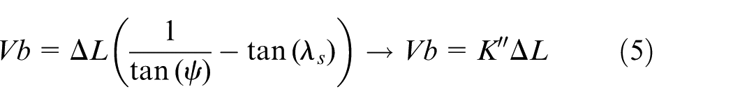
The model relating the change in tool length to tool flank wear was derived geometrically using Figure 4 and is shown in equation (5), where ψ and λ_s are the geometrical properties of the insert which generate the constant K″, and ΔL is the change in tool length after the cutting process. Note that only axial change in the tool length has been considered in this work and the radial change has been neglected

Vb = Δ L (\frac{1}{\tan (ψ)} - \tan (λ_{s})) \to Vb = K ″ Δ L

(5)

Figure 4.

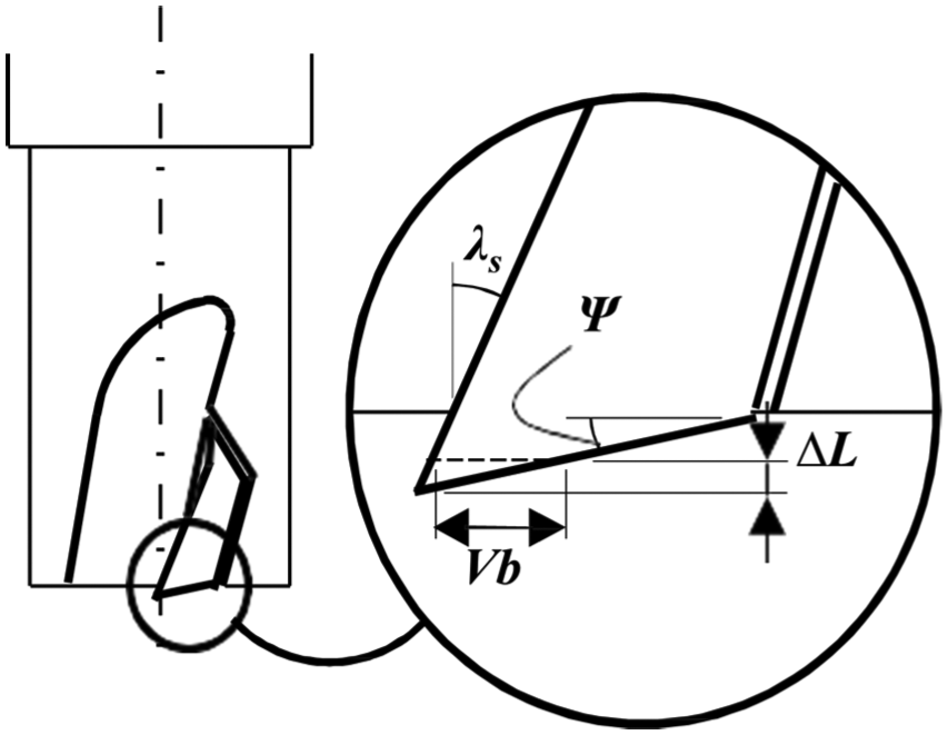
Insert geometry.²³

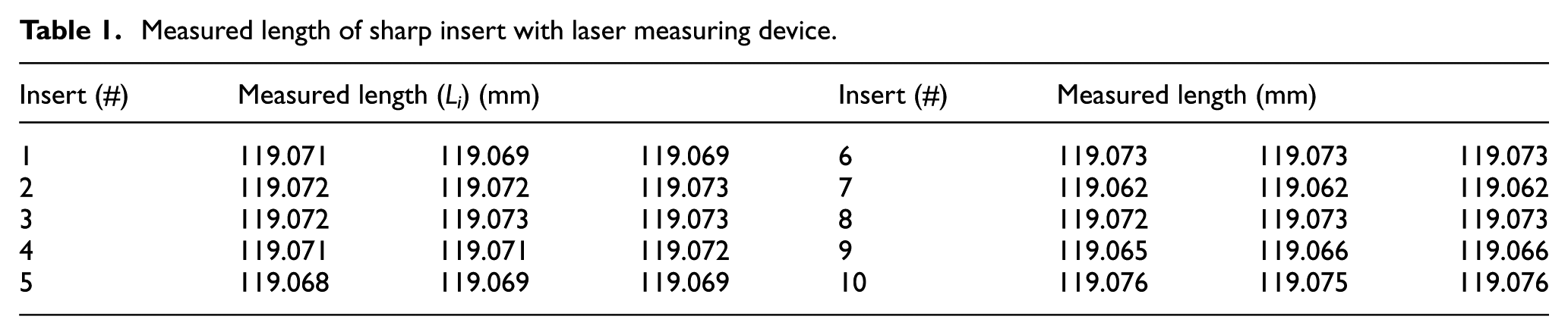
To obtain the accuracy of the measurement system, a statistical gage R&R was carried out for 10 randomly selected new inserts. The length of each insert was measured three times and total of 3 × 10 = 30 data points were obtained (see Table 1). Since one measurement device existed, only repeatability can be evaluated and reproducibility cannot be evaluated here with gage R&R. From the total %variation shown in Table 2, 14.93% was attributed to the gage system. This value is considered as accepted according to Automotive Industry Action Group (AIAG) criteria (>30% is a threshold for rejection) and proves the accuracy of the measuring system (laser measurement device) and shows the largest cause of variation is rooted in insert’s geometrical tolerances.

Table 1.

Measured length of sharp insert with laser measuring device.

Insert (#)	Measured length (L_i) (mm)			Insert (#)	Measured length (mm)
1	119.071	119.069	119.069	6	119.073	119.073	119.073
2	119.072	119.072	119.073	7	119.062	119.062	119.062
3	119.072	119.073	119.073	8	119.072	119.073	119.073
4	119.071	119.071	119.072	9	119.065	119.066	119.066
5	119.068	119.069	119.069	10	119.076	119.075	119.076

Table 2.

Gage R&R results for evaluating amount of variation in measuring system.

Source	SD	Study variation (6 × SD)	% Study variation
Total gage R&R	0.0006055	0.0036332	14.93
Repeatability	0.0006055	0.0036332	14.93
Reproducibility	N/A
Part-to-part	0.0040108	0.0240647	98.88
Total variation	0.0040562	0.0243374	100.00

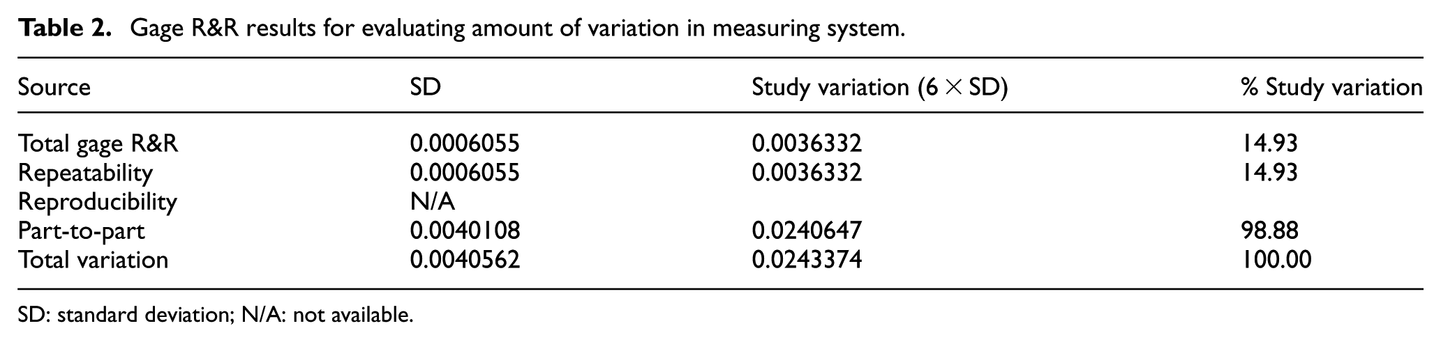
SD: standard deviation; N/A: not available.

Experimental setup

Rene-108 Ni-based alloy is chosen in this work as the workpiece material. A down-milling operation with 2 flute Sandvik R390-11 T3 08M-PM 1030, TiAlN-coated insert with 60% engagement was performed on the rectangular block of size 60 × 80 × 25 mm with Okuma GENOS M460-VE three-axis CNC. Wet machining is chosen as the lubrication strategy to avoid early failure of the insert due to the poor machinability of the chosen material. The workpiece installation and test setup configuration in the CNC machine are shown in Figure 5.

Figure 5.

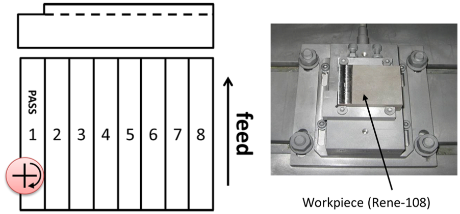
Workpiece (Rene-108) test setup.

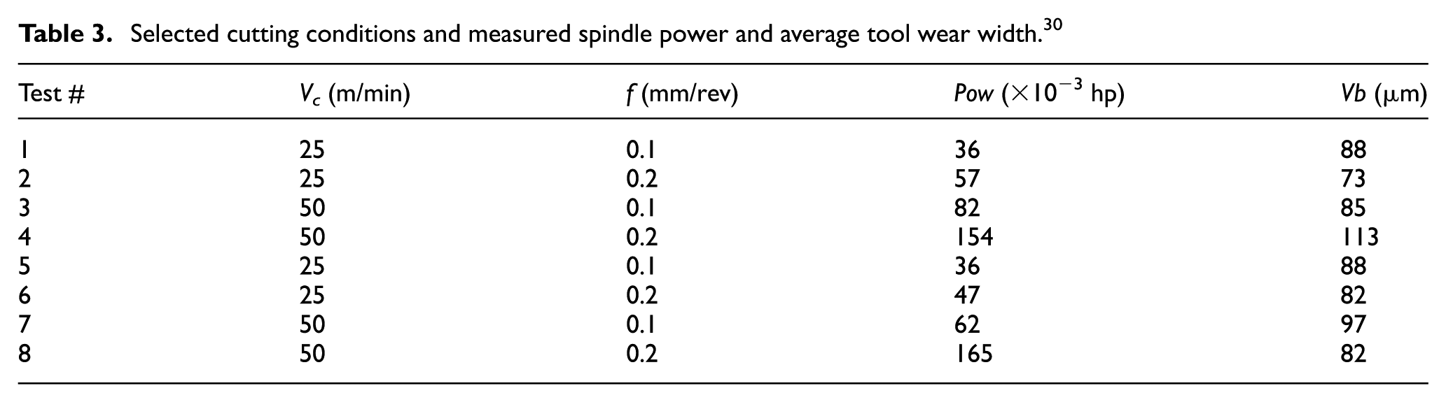
To identify and calibrate the unknown parameters K_i in equation (4), four sets of experiments with two replications were carried out in variable feed and cutting speed and constant cutting depth of 0.5 mm. In each experiment, a sharp insert was used and the average tool wear width was measured on the flank side of the insert using an optical microscope in addition to the average spindle power between 80% and 90% of the total cutting distance as shown in Table 3.

Table 3.

Selected cutting conditions and measured spindle power and average tool wear width.³⁰

Test #	V_c (m/min)	f (mm/rev)	Pow (×10⁻³ hp)	Vb (µm)
1	25	0.1	36	88
2	25	0.2	57	73
3	50	0.1	82	85
4	50	0.2	154	113
5	25	0.1	36	88
6	25	0.2	47	82
7	50	0.1	62	97
8	50	0.2	165	82

Identifying mechanisms of the tool wear

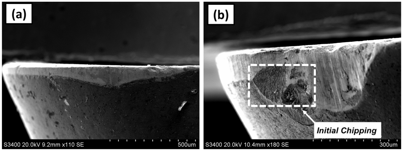
To shed a light on tool failure mechanisms in end-milling of Rene-108, scanning electron microscopy (SEM) along with X-ray elemental analysis were used to study the flank side of the insert in different cutting conditions. As shown in Figure 6(a), the elemental analysis showed an extensive amount of nickel and cobalt on the flank face of the insert in the mildest feed and cutting speed, which represents adhesion and diffusion wear mechanisms in the cutting process. Parallel grooves on the flank face were also observed, which represent abrasion wear. With an increase in feed, initial chipping of coating was observed in Figure 6(b). High content of tungsten which is the base material for the insert revealed the initiation of coating damage during the cutting process. Considering Figure 6(c), where only cutting speed is increased shows a larger chipped off area from the flank face; therefore, it can be concluded that cutting speed has more influence on exciting the chipping mechanism in the process. In the most aggressive cutting condition, where both feed and cutting speed increased together, extensive chipping was observed. The SEM image in Figure 6(d) demonstrates a completely failed insert in these cutting conditions. The existence of each wear failure mode is summarized graphically in Table 4. It is clear that chipping starts in the first pass except for the mildest conditions.

Figure 6.

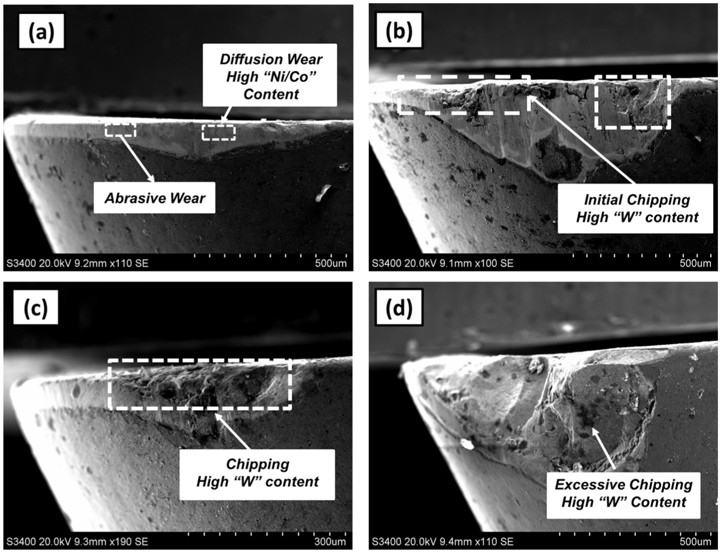
SEM image for (a) feed of 0.1 mm/rev and cutting speed of 25 mm/min, (b) feed of 0.2 mm/rev and cutting speed of 25 mm/min, (c) feed of 0.1 mm/rev and cutting speed of 50 mm/min, and (d) feed of 0.2 mm/rev and cutting speed of 50 mm/min.³⁰

Table 4.

Contribution of dominant tool failure modes in different cutting conditions in milling Rene-108.

	Feed (mm/rev)	Cutting speed (m/min)
1	0.1	25
2	0.2	25
3	0.1	50
4	0.2	50

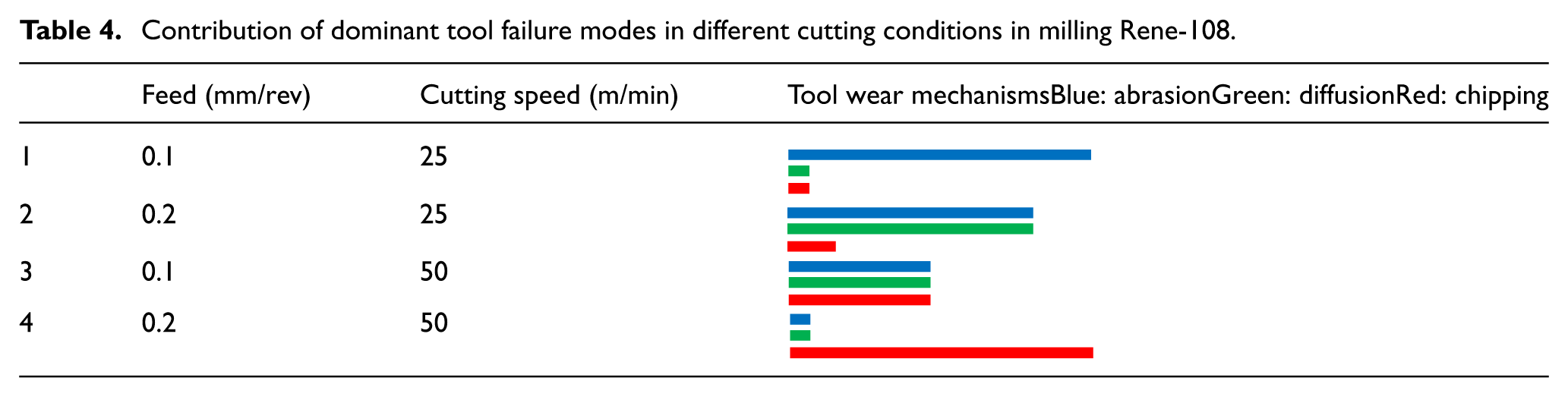
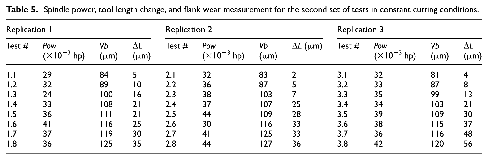
In this study, Table 3 was used solely for offline inference on the unknown parameters of the power model in equation (4). For the rest of the study, it was decided to choose a certain feed and cutting speed to avoid or delay the chipping effect. Therefore, for online stochastic estimation, it was decided to run three replications with constant cutting conditions (feed 0.1 mm/rev and speed of 25 mm/min). Each replication started with a sharp insert and continued with the same insert until extensive chipping was observed. After only eight consecutive cuts, the insert reached a failure region as shown in Figure 7, where chipped off coating can be observed in Figure 7(b). In addition to spindle power, the length of the cutting tool was measured three times before and after each cut, and the average tool length change was calculated. In Table 5, the measured power and the tool length change for each cut are shown. As illustrated in Figure 8, the linear regression analysis between tool flank wear width and tool length change shows 97%, 86%, and 89% goodness of fit (R²) for each replication. Therefore, the linear geometrical relation of equation (5) is in agreement with the experimental results.

Figure 7.

Progress of the tool flank wear from the (a) first cut to (b) eighth cut.

Table 5.

Spindle power, tool length change, and flank wear measurement for the second set of tests in constant cutting conditions.

Replication 1				Replication 2				Replication 3
Test #	Pow (×10⁻³ hp)	Vb (µm)	ΔL (µm)	Test #	Pow (×10⁻³ hp)	Vb (µm)	ΔL (µm)	Test #	Pow (×10⁻³ hp)	Vb (µm)	ΔL (µm)
1.1	29	84	5	2.1	32	83	2	3.1	32	81	4
1.2	32	89	10	2.2	36	87	5	3.2	33	87	8
1.3	24	100	16	2.3	38	103	7	3.3	35	99	13
1.4	33	108	21	2.4	37	107	25	3.4	34	103	21
1.5	36	111	21	2.5	44	109	28	3.5	39	109	30
1.6	41	116	25	2.6	30	116	33	3.6	38	115	37
1.7	37	119	30	2.7	41	125	33	3.7	36	116	48
1.8	36	125	35	2.8	44	127	36	3.8	42	120	56

Figure 8.

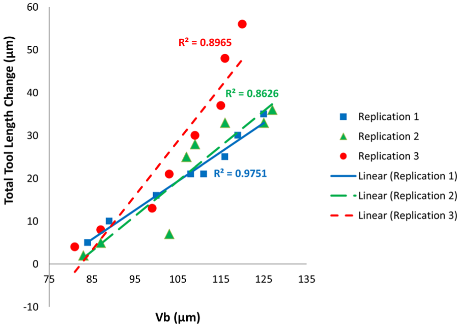
Linear regression analysis on experimental results of tool length change and average flank wear width.

Random-walk Metropolis method for inference on cutting power model

To make an inference on parameters K_i of equation (4) the Bayesian random-walk Metropolis algorithm was chosen. This has been discussed in the previous work of Akhavan Niaki et al.³⁰ and will be briefly discussed here. To highlight the advantage of this method over the Frequentist maximum likelihood method, a small dataset of Table 3 with only eight experiments was used. It is a reasonable assumption to initialize the Markov chain with the output of Frequentist maximum likelihood method. Hence, parameters K₁, K₂, and K₃ were found using the simplex unconstrained search algorithm shown in equation (6), and the Markov chain started with them

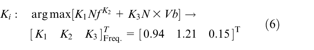
\begin{array}{l} K_{i} : \arg \max [K_{1} N f^{K_{2}} + K_{3} N \times V b] \to \\ [\begin{matrix} K_{1} & K_{2} & K_{3} \end{matrix}]_{Freq .}^{T} = [\begin{matrix} 0.94 & 1.21 & 0.15 \end{matrix}]^{T} \end{array}

(6)

The method proposed by Solonen³⁴ is chosen for finding the initial proposal density covariance (δ²) using the Jacobian matrix of unknown parameters. To improve the performance of the random-walk method, the algorithm was run twice, first with 2000 samples and then with 10,000 samples. The initial prior of the second chain was updated using the mean and covariance of the generated chain in the first run. The output as the probabilistic distribution of each pair of parameters K_i using Bayesian-based method is shown in Figure 9. The expected value of the unknown parameters shown in equation (7) is different from what the Frequentist maximum likelihood method estimated (see equation (6)). This difference is attributed to the searching algorithm of Frequentist method, where it only identifies the local maxima of a function. On the other hand, the random-walk Metropolis method is capable of bringing additional information as the initial prior to the search domain, which makes it more robust in finding the global maxima. This becomes specifically significant when limited information is available for inference. The effect of using identified parameters with the Bayesian or Frequentist approaches on the online estimation accuracy will be discussed in section “Results and discussion”

E ([\begin{matrix} K_{1} & K_{2} & K_{3} \end{matrix}]_{Bayes .}^{T}) = [\begin{matrix} 1.94 & 1.79 & 0.43 \end{matrix}]^{T}

(7)

Figure 9.

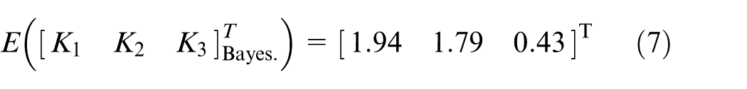
Identified probability of parameters after running the random-walk Metropolis algorithm: (a) K₁ − K₂, (b) K₂ − K₃, and (c) K₁ − K₃.³⁰

Stochastic modeling of tool flank wear

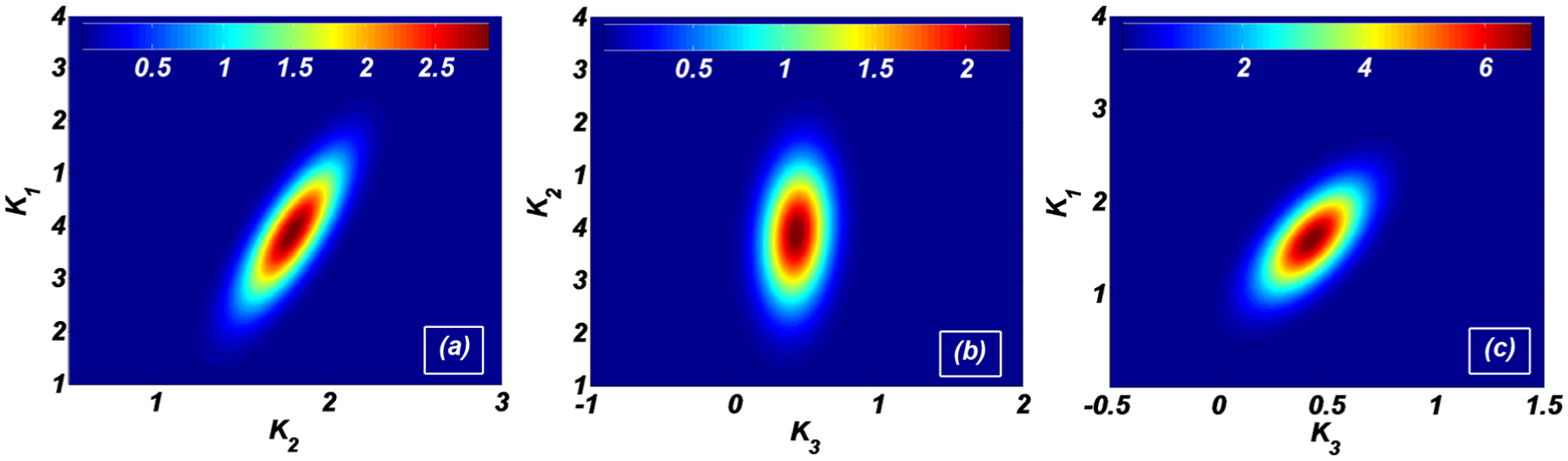
To study the online estimation performance using the Kalman filter, information from Table 5 was used. Due to poor machinability of the selected material (Rene-108), the evolution of tool flank wear was very fast as described in section “Identifying mechanisms of the tool wear” where only eight cuts could be completed before excessive chipping. To enable the in-process tool wear monitoring, spindle power and tool length were measured in five distinct regions of each cut. However, the tool wear was measured at the end of each cut, and therefore, for each five measurements, one actual value of the tool wear existed. Considering a linear progress for the tool wear and assuming it as the first state of the system, the tool wear rate was assumed as the second state. Hence, a discretized state model can be written as equation (8), where MR denotes the volume of removed material. The state errors were added to equation (7) as two independent normally distributed zero-mean noises with variances q₁ and q₂, respectively

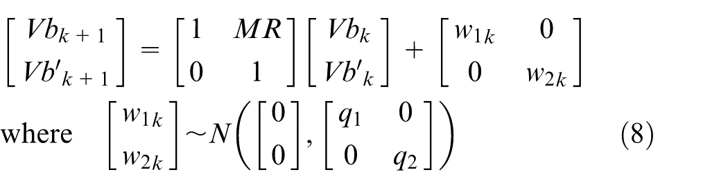
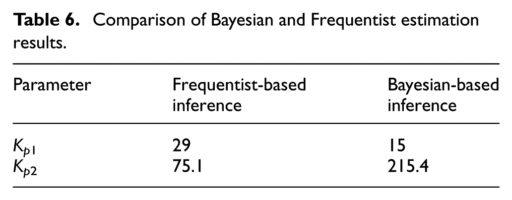
[\begin{matrix} V b_{k + 1} \\ V {b^{'}}_{k + 1} \end{matrix}] = [\begin{matrix} 1 & M R \\ 0 & 1 \end{matrix}] [\begin{matrix} V b_{k} \\ V {b^{'}}_{k} \end{matrix}] + [\begin{matrix} w_{1 k} & 0 \\ 0 & w_{2 k} \end{matrix}] where [\begin{matrix} w_{1 k} \\ w_{2 k} \end{matrix}] \sim N ([\begin{matrix} 0 \\ 0 \end{matrix}], [\begin{matrix} q_{1} & 0 \\ 0 & q_{2} \end{matrix}])

(8)

The maximum variances of the measured tool wear and the tool wear rate determine the approximate values for the state noise variances (q_i). These were calculated as q₁ = 1.36 × 10² µm² and q₂ = 1.6 × 10⁻⁶ µm²/mm⁶. Constant cutting conditions simplify equation (4) as equation (9). The parameters K_p₁ and K_p₂ were determined from the results of Bayesian and Frequentist methods described in section “Random-walk Metropolis method for inference on cutting power model.” These parameters are shown in Table 6

Pow = K_{p 1} + K_{p 2} Vb

(9)

Table 6.

Comparison of Bayesian and Frequentist estimation results.

Parameter	Frequentist-based inference	Bayesian-based inference
K_p ₁	29	15
K_p ₂	75.1	215.4

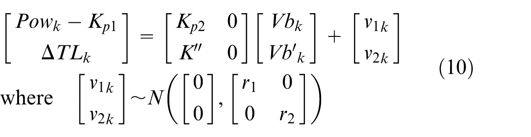
The measurement error variances for the spindle power and tool length change were calculated the same way as q₁ equal to 11.3 hp² and 14 × 10² µm², respectively, and equation (9) was re-written in discrete format as equation (10) with the assumption of independent measurements. For further discussion on selection of initial states and covariance matrices, refer to Akhavan Niaki et al.²⁴

[\begin{matrix} P o w_{k} - K_{p 1} \\ Δ T L_{k} \end{matrix}] = [\begin{matrix} K_{p 2} & 0 \\ K^{″} & 0 \end{matrix}] [\begin{matrix} V b_{k} \\ V {b^{'}}_{k} \end{matrix}] + [\begin{matrix} v_{1 k} \\ v_{2 k} \end{matrix}] where [\begin{matrix} v_{1 k} \\ v_{2 k} \end{matrix}] \sim N ([\begin{matrix} 0 \\ 0 \end{matrix}], [\begin{matrix} r_{1} & 0 \\ 0 & r_{2} \end{matrix}])

(10)

Results and discussion

Performance of the Kalman filter using indirect measurement

As described in Figure 2, Bayesian and Frequentist models were fed as the measurement model in the Kalman filter. The Kalman filter’s outputs using these two approaches are shown in Figures 10 and 11. A significant error reduction in the output of the Kalman filter was observed when a Bayesian-based model was used as the measurement model. However, unlike the measured tool wear, the estimated wear does not exhibit a linear monotonically increasing function specifically for first and second replications of Figure 11. This behavior is attributed to insert chipping. When small pieces of the insert coating chip off from the flank face during the operation, a sudden drop followed by a rise in the power signal can be observed. Since the chipped particle at the tool tip reduces the contact area between the flank face and the workpiece, the power cannot reach the same magnitude when previous surfaces were in full contact. This effect shown in Figure 12 affects the estimated flank wear, causing an unrealistic drop in the estimated wear. Note that the Kalman filter estimates the mean and covariance of the states, and therefore, uncertainty in Figures 10 and 11 represents the variance of estimated tool wear; the evolution of the tool wear represented by the Gaussian function is shown in Figure 13.

Figure 10.

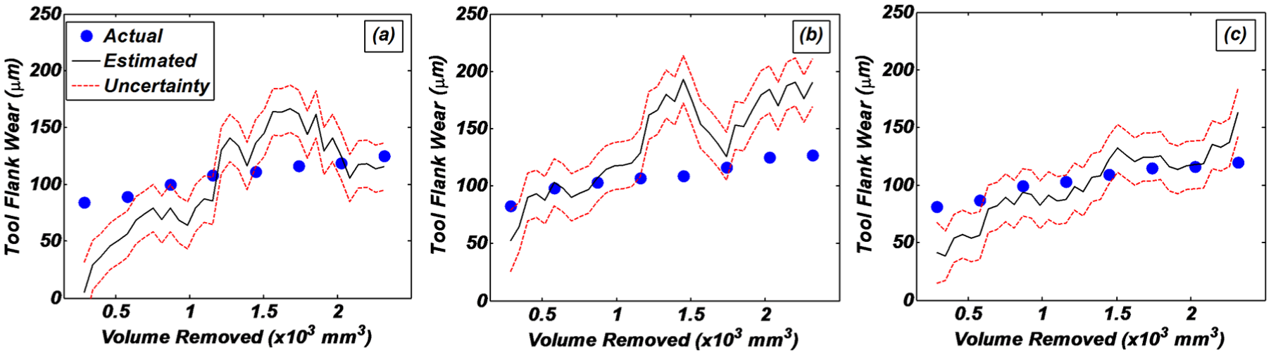
Estimated tool flank wear and its corresponding uncertainty when Frequentist-based power model is used: (a) first replication, (b) second replication, and (c) third replication.

Figure 11.

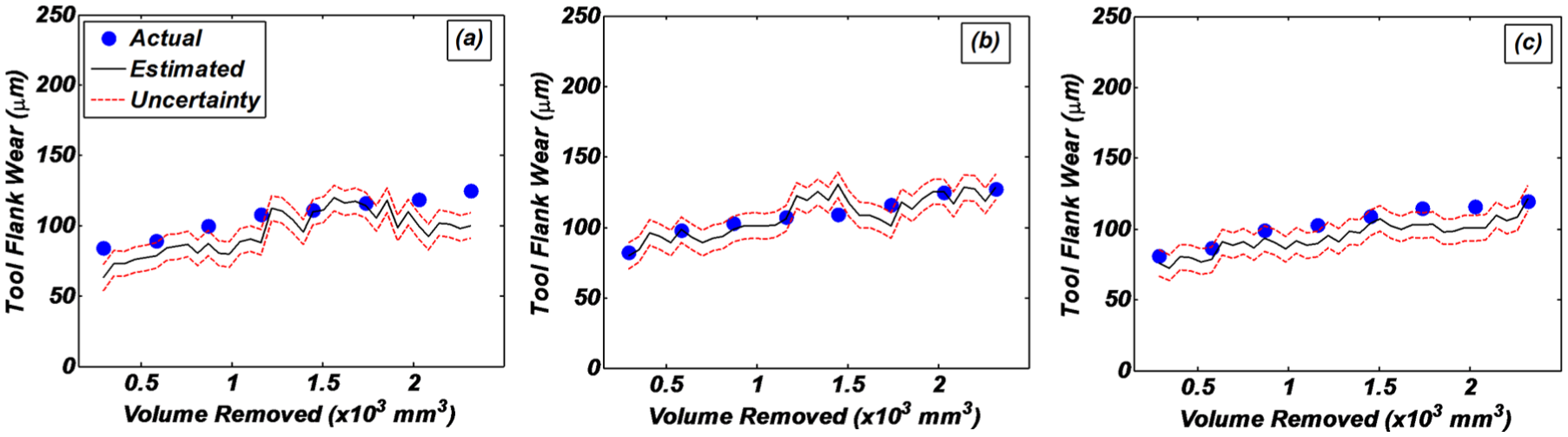
Estimated tool flank wear and its corresponding uncertainty when Bayesian-based power model is used: (a) first replication, (b) second replication, and (c) third replication.

Figure 12.

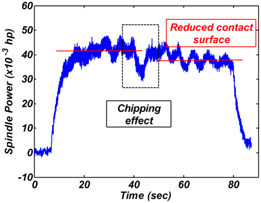
Chipping effect as drop and rise in power signal for test 1.7.

Figure 13.

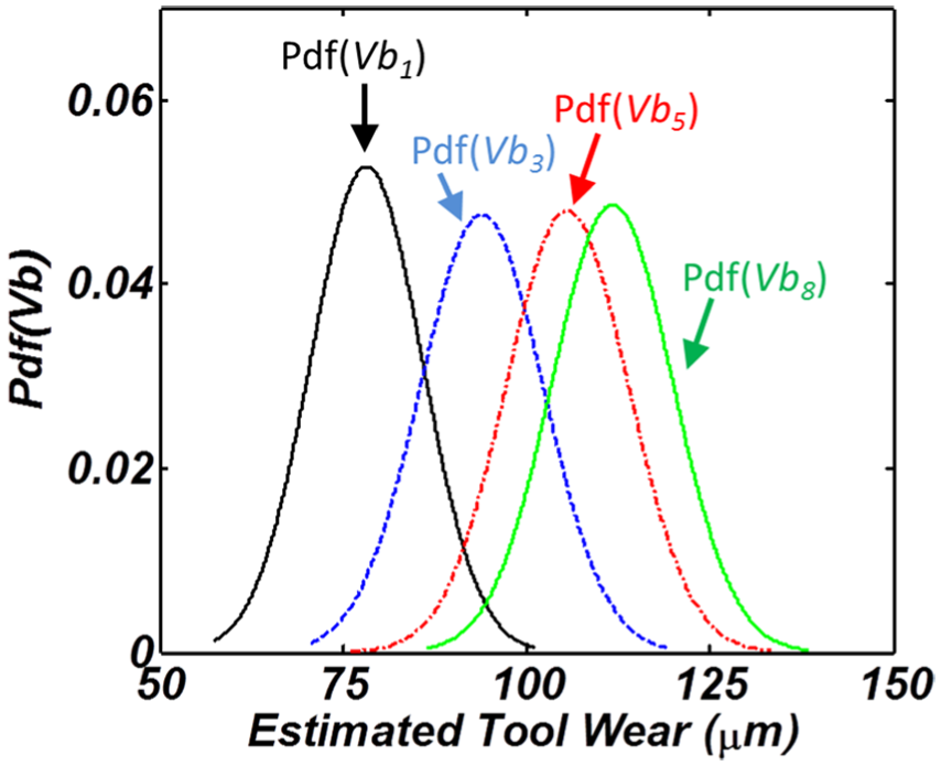
Evolution of tool wear probability distribution over time for the first replication (with Bayesian-based measurement model).

Feasibility of fusing direct and indirect measurement

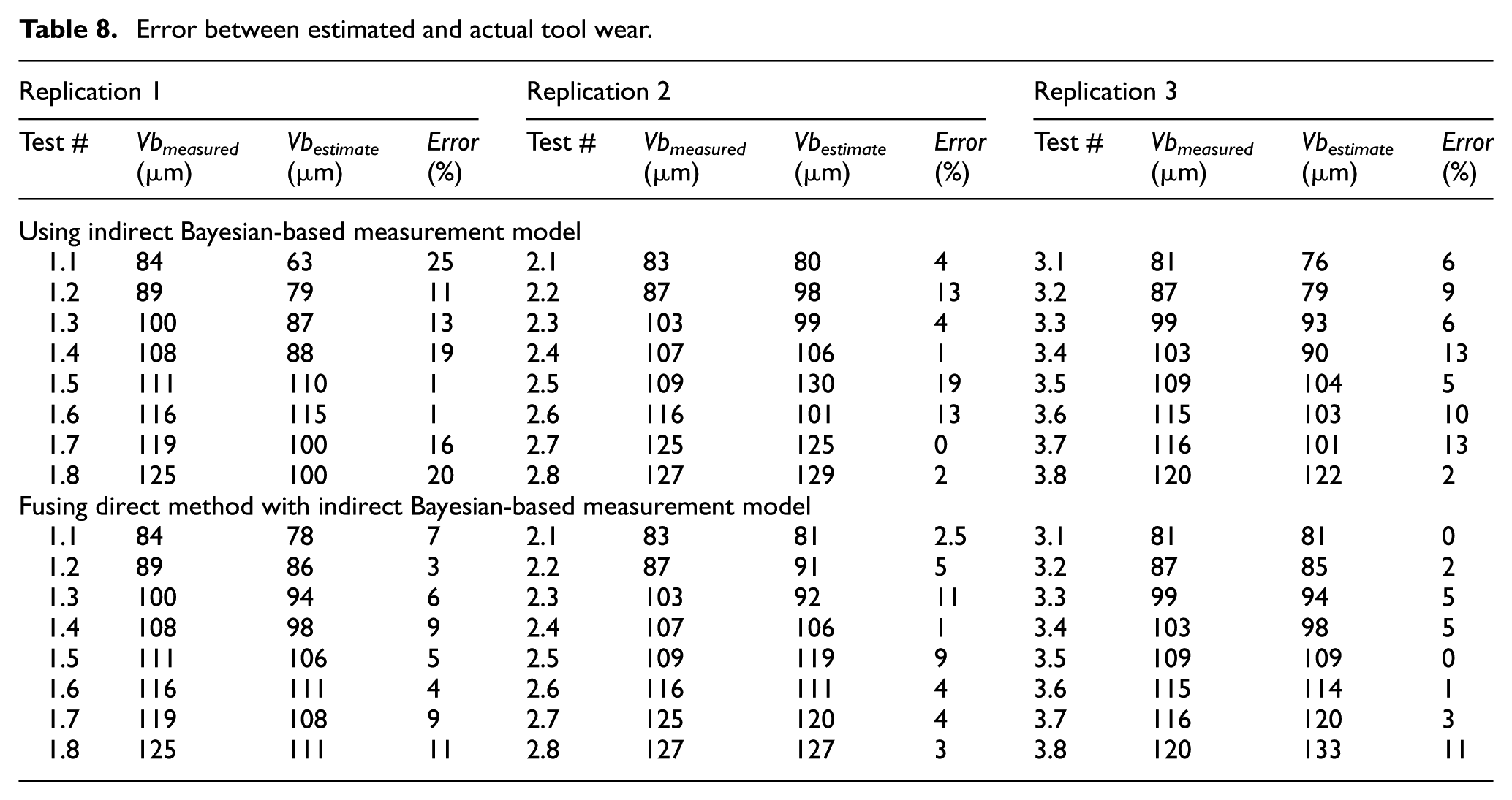
Using a laser measuring system to capture the change in tool length provides direct access to the tool wear. The information from this system can easily be fused with the power signal in the Kalman filter framework as shown in equation (10). The results of estimation are shown in Figure 14, where significant improvement was observed. Furthermore, the chipping effect was significantly compensated. To evaluate the improvement of fusing direct method into the indirect method (using only power signal), three errors were selected: root mean square error (RMSE), mean absolute error (MAE), and maximum error and compared in Table 7. Moreover, the percentage errors between the estimated wear and the actual wear for all the replications are compared in Table 8.

Figure 14.

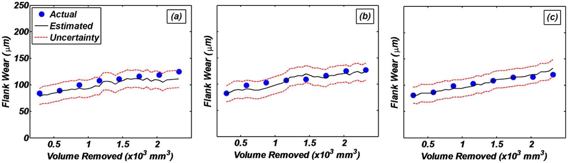
Estimated tool flank wear and its corresponding uncertainty when direct and indirect method fused together: (a) first replication, (b) second replication, and (c) third replication.

Table 7.

Error comparison for each replication.

Method	Replication 1			Replication 2			Replication 3
Method	RMSE	MAE	Max. error	RMSE	MAE	Max. error	RMSE	MAE	Max. error
Freq.-based model	11.1	30.4	79.6	27.1	34.7	83.8	3.1	19.8	43.2
Bayes.-based model	13.8	13.8	25.0	0.06	5.7	21.2	7.9	8.3	15.1
Fusion with direct measurement	7.5	7.4	11.2	5.4	5.4	10.7	3.7	3.7	10.9

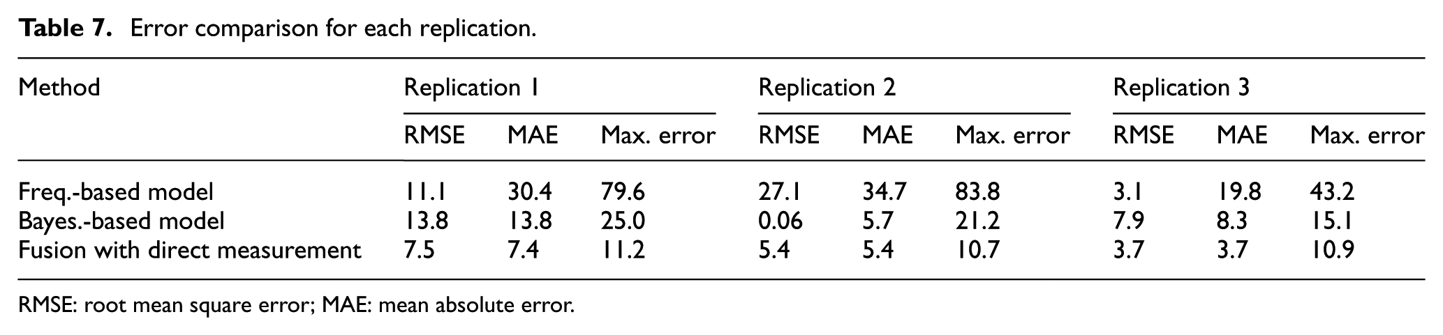
RMSE: root mean square error; MAE: mean absolute error.

Table 8.

Error between estimated and actual tool wear.

Replication 1				Replication 2				Replication 3
Test #	Vb_measured (µm)	Vb_estimate (µm)	Error (%)	Test #	Vb_measured (µm)	Vb_estimate (µm)	Error (%)	Test #	Vb_measured (µm)	Vb_estimate (µm)	Error (%)
Using indirect Bayesian-based measurement model
1.1	84	63	25	2.1	83	80	4	3.1	81	76	6
1.2	89	79	11	2.2	87	98	13	3.2	87	79	9
1.3	100	87	13	2.3	103	99	4	3.3	99	93	6
1.4	108	88	19	2.4	107	106	1	3.4	103	90	13
1.5	111	110	1	2.5	109	130	19	3.5	109	104	5
1.6	116	115	1	2.6	116	101	13	3.6	115	103	10
1.7	119	100	16	2.7	125	125	0	3.7	116	101	13
1.8	125	100	20	2.8	127	129	2	3.8	120	122	2
Fusing direct method with indirect Bayesian-based measurement model
1.1	84	78	7	2.1	83	81	2.5	3.1	81	81	0
1.2	89	86	3	2.2	87	91	5	3.2	87	85	2
1.3	100	94	6	2.3	103	92	11	3.3	99	94	5
1.4	108	98	9	2.4	107	106	1	3.4	103	98	5
1.5	111	106	5	2.5	109	119	9	3.5	109	109	0
1.6	116	111	4	2.6	116	111	4	3.6	115	114	1
1.7	119	108	9	2.7	125	120	4	3.7	116	120	3
1.8	125	111	11	2.8	127	127	3	3.8	120	133	11

Effect of measurement noise on the performance of the filter

The uncertainty of the tool wear probability distribution (estimated variance P_k in equation (3)) after using each method described in sections “Performance of the Kalman filter using indirect measurement” and “Feasibility of fusing direct and indirect measurement” is shown in Figure 15. It is worthwhile mentioning that while adding the information from the laser measuring system improved the estimation accuracy in terms of RMSE and MAE, the uncertainty of the estimation increased. This is due to the selection of measurement noise for the laser system. The focus of this work was to reduce the estimation error; therefore, the measurement noise variance (r₂ in equation (10)) was tuned to produce the least RMSE. The trade-off between estimation error and uncertainty in the results is shown in Figure 16. By decreasing the measurement noise variance r₂, less uncertainty in the output was achieved. However, the RMSE of the outputs increased for the second and third replications. On the other hand, by increasing the measurement noise variance from the current chosen condition (m = 1 in Figure 16), both uncertainty and RMSE increased for the first and third replications, while the RMSE of the second replication remained almost constant and the filter failed to produce reliable results. Therefore, fine-tuning of the filter parameters plays a significant role in the output results.

Figure 15.

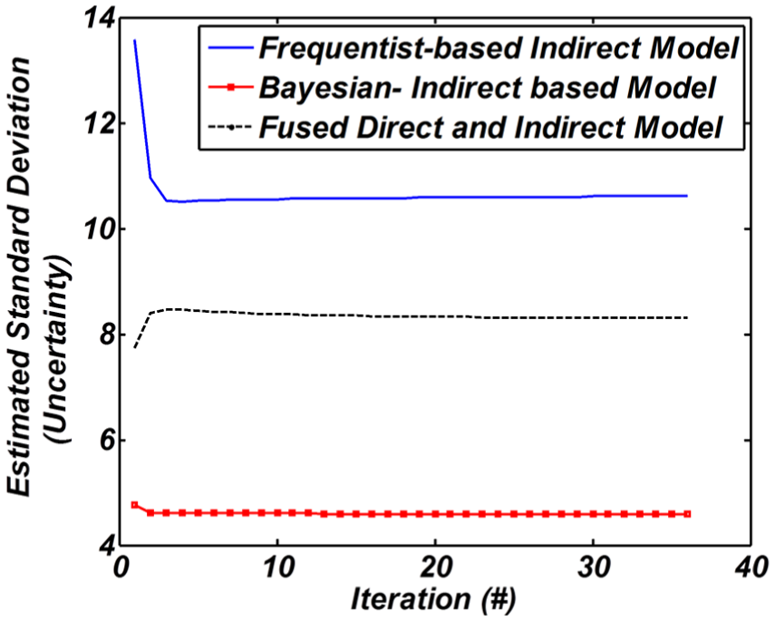
Evolution of estimated tool wear uncertainty (P_k) using different methods, adding direct laser measurement increased the uncertainty but decreased RMSE.

Figure 16.

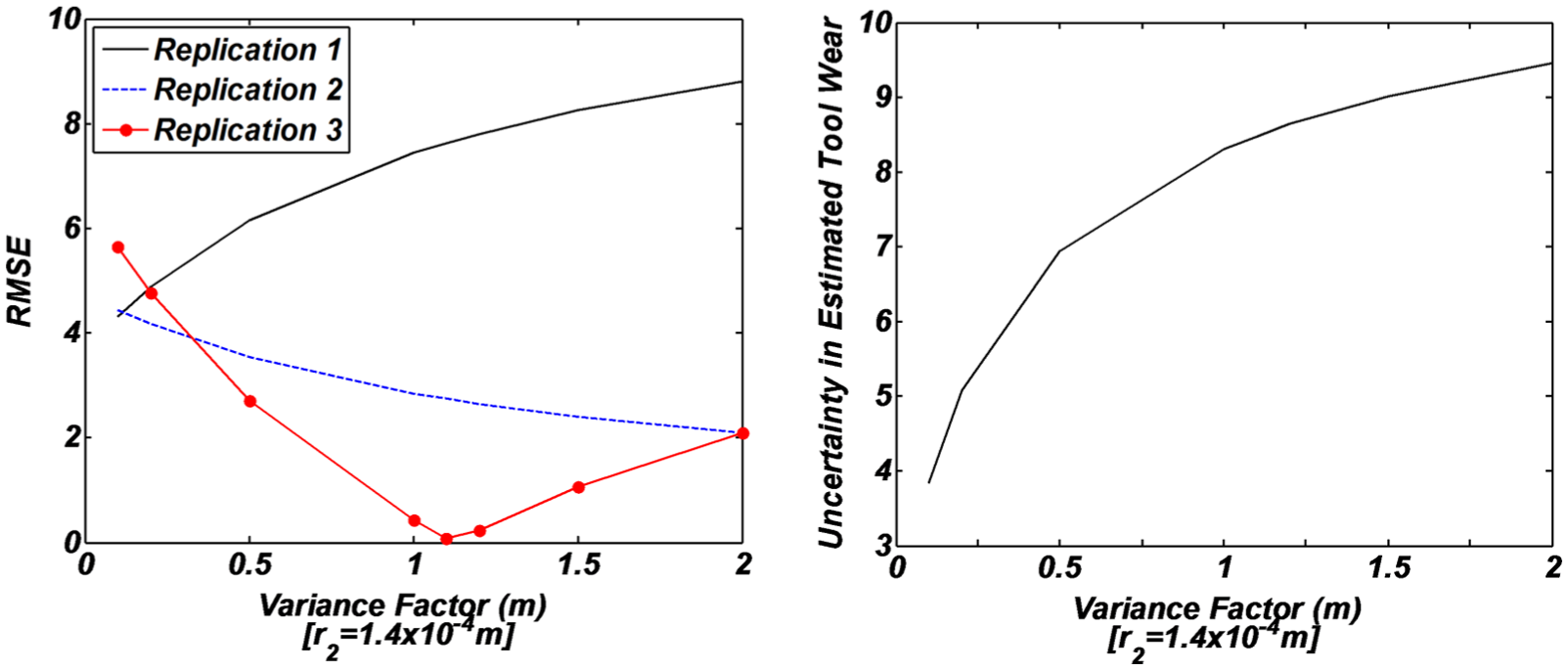
Trade-off between uncertainty in the output and estimation error.

Conclusion

In this work, a probabilistic-based method was used to first estimate the average flank wear in end-milling Rene 108 difficult-to-machine alloy and second to identify the uncertainties in estimated wear. Furthermore, the possibility of introducing direct laser measuring method to improve the estimation was discussed. The following are the takeaways from this study:

The dominant tool failure mechanisms existing in milling Rene-108 were identified using SEM image and elemental analysis, and proper cutting conditions were selected to delay chipping at the initial stages of tool wear progress. It was concluded that with an increase in cutting speed, the dominant wear mechanism evolves from adhesion and diffusion to chipping.

Random-walk Metropolis algorithm as a Bayesian parameter inference method was used and its performance against Frequentist maximum likelihood estimation was investigated when a limited dataset is available for inference. It was shown that using the Bayesian-based model outweighs the Frequentist-based model when it is used in the Kalman filter framework.

To increase the performance of the filter, intermittent direct measurement from the laser measuring system was added to the Kalman filter. The accuracy of the estimation was compared when using only spindle power and it was shown that significant improvement can be achieved using this method. It was discussed that the chosen direct method does not require human interference and conserves the automatic estimation platform for monitoring the tool wear.

This work provides valuable information about the evolution of probability distribution of the tool wear during the cutting process in terms of average wear and its corresponding uncertainty. In high-value industrial applications, preserving the quality of the workpiece comes before saving the tool. On the other hand, the focus of academia is solely on the tool wear. Therefore, the missing gap still exists between the beneficial/detrimental effects of tool wear on the surface quality and a proper decision-making strategy for stopping the process to preserve the quality of the part. The decision-making strategy should be sensitive not only to the tool wear but also to the underlying uncertainty as well. Investigating such methods is worthy of future studies.

Footnotes

Appendix 1 Acknowledgements

Any opinions, findings, and conclusions or recommendations expressed in this material are those of the authors and do not necessarily reflect the views of the National Science Foundation.

Declaration of conflicting interests

The author(s) declared no potential conflicts of interest with respect to the research, authorship, and/or publication of this article.

Funding

The author(s) disclosed receipt of the following financial support for the research, authorship, and/or publication of this article: The authors wish to thank the National Science Foundation for support of this work under Grant No. 0954318.

References

Vallejo

Jr Nolazco-Flores

Morales-Menéndez

et al . Tool-wear monitoring based on continuous hidden Markov models. In: Proceedings of the 10th Ibero American congress conference on progress in pattern recognition, image analysis and applications, Havana, Cuba, 15–18 November 2005, pp.880–890. Berlin: Springer.

Atli

Urhan

Ertürk

et al . A computer vision-based fast approach to drilling tool condition monitoring. Proc IMechE, Part B: J Engineering Manufacture 2006; 220(9): 1409–1415.

Arunachalam

Ramamoorthy

Texture analysis for grinding wheel wear assessment using machine vision. Proc IMechE, Part B: J Engineering Manufacture 2007; 221(3): 419–430.

Dutta

Pal

Mukhopadhyay

et al . Application of digital image processing in tool condition monitoring: a review. CIRP J Manuf Sci Technol 2013; 6(3): 212–232.

Sortino

Application of statistical filtering for optical detection of tool wear. Int J Mach Tool Manu 2003; 43(5): 493–497.

Shahabi

Ratnam

Assessment of flank wear and nose radius wear from workpiece roughness profile in turning operation using machine vision. Int J Adv Manuf Tech 2009; 43(1–2): 11–21.

Kuttolamadom

Mears

Kurfess

TR.

On the volumetric assessment of tool wear in machining inserts with complex geometries—part 1: need, methodology, and standardization. J Manuf Sci Eng 2012; 134(5): 051002.

Kuttolamadom

Mehta

Mears

et al . Correlation of the volumetric tool wear rate of carbide milling inserts with the material removal rate of Ti–6Al–4V. J Manuf Sci Eng 2015; 137(2): 021021-1–021021-8.

Taylor

FW.

The art of cutting metals. Sci Am 1907; 63: 25942–25944.

10.

Srikant

Krishna

Rao

Online tool wear prediction in wet machining using modified back propagation neural network. Proc IMechE, Part B: J Engineering Manufacture 2011; 225: 1009–1018.

11.

Paul

Varadarajan

A multi-sensor fusion model based on an artificial neural network to predict tool wear during hard turning. Proc IMechE, Part B: J Engineering Manufacture 2012; 226(5): 853–860.

12.

Kaya

Oysu

Ertunc

et al . A support vector machine-based online tool condition monitoring for milling using sensor fusion and a genetic algorithm. Proc IMechE, Part B: J Engineering Manufacture 2012; 226(11): 1808–1818.

13.

Schmitz

Karandikar

Kim

et al . Uncertainty in machining: workshop summary and contributions. J Manuf Sci Eng 2011; 133(5): 051009.

14.

Karandikar

Abbas

Schmitz

TL.

Tool life prediction using Bayesian updating. Part 1: milling tool life model using a discrete grid method. Precis Eng 2014; 38(1): 9–17.

15.

Karandikar

Abbas

Schmitz

TL.

Tool life prediction using Bayesian updating. Part 2: turning tool life using a Markov Chain Monte Carlo approach. Precis Eng 2014; 38(1): 18–27.

16.

Dey

Stori

A Bayesian network approach to root cause diagnosis of process variations. Int J Mach Tool Manu 2005; 45(1): 75–91.

17.

Karandikar

McLeay

Turner

et al . Tool wear monitoring using naïve Bayes classifiers. Int J Adv Manuf Tech 2015; 77(9–12): 1613–1626.

18.

Mehta

Werner

Mears

Condition based maintenance-systems integration and intelligence using Bayesian classification and sensor fusion. J Intell Manuf 2015; 26(2): 331–346.

19.

Rabiner

A tutorial on hidden Markov models and selected applications in speech recognition. P IEEE 1989; 77(2): 257–286.

20.

Zhu

Wong

Hong

GS.

Multi-category micro-milling tool wear monitoring with continuous hidden Markov models. Mech Syst Signal Pr 2009; 23(2): 547–560.

21.

Wang

CHMM for tool condition monitoring and remaining useful life prediction. Int J Adv Manuf Tech 2012; 59(5–8): 463–471.

22.

Scheffer

Engelbrecht

Heyns

A comparative evaluation of neural networks and hidden Markov models for monitoring turning tool wear. Neural Comput Appl 2005; 14(4): 325–336.

23.

Henderson

Updated force model for milling nickel-based superalloys. PhD Dissertation, Clemson University, Clemson, SC, 2012.

24.

Akhavan Niaki

Ulutan

Mears

. Stochastic tool wear assessment in milling difficult to machine alloys. Int J Mechatron Manuf Syst 2015; 8(3–4): 134–159.

25.

Akhavan Niaki

Michel

Mears

. State of health monitoring in machining: extended Kalman filter for tool wear assessment in turning of IN718 hard-to-machine alloy. J Manuf Process 2016; 24: 361–369.

26.

Wang

Gao

RX.

Markov nonlinear system estimation for engine performance tracking. J Eng Gas Turb Power 2016; 138(9): 091201.

27.

Wang

Gao

RX.

Stochastic tool wear prediction for sustainable manufacturing. Proced CIRP 2016; 48: 236–241.

28.

Akhtar

Sun

et al . Tool wear mechanisms in the machining of nickel based super-alloys: a review. Front Mech Eng 2014; 9(2): 106–119.

29.

Thakur

Gangopadhyay

State-of-the-art in surface integrity in machining of nickel-based super alloys. Int J Mach Tool Manu 2016; 100: 25–54.

30.

Akhavan Niaki

Ulutan

Mears

. Parameter inference under uncertainty in end-milling γ′-strengthened difficult-to-machine alloy. J Manuf Sci Eng 2016; 138(6): 061014-1–061014-10.

31.

Shao

Wang

Zhao

XM.

A cutting power model for tool wear monitoring in milling. Int J Mach Tool Manu 2004; 44(14): 1503–1509.

32.

Mohammadi

Ravindra

Kode

et al . Experimental work on micro laser-assisted diamond turning of silicon (111). J Manuf Process 2015; 19: 125–128.

33.

Mohammadi

Bogaç Poyraz

Ravindra

et al . Surface finish improvement of an unpolished silicon wafer using micro-laser assisted machining. Int J Abras Technol 2015; 7(2): 107–121.

34.

Solonen

Monte Carlo methods in parameter estimation of nonlinear model. Master’s Thesis, Lappeenranta University of Technology, Lappeenranta, 2006.

Test #	V_c (m/min)	f (mm/rev)	Pow (×10⁻³ hp)	Vb (µm)
1	25	0.1	36	88
2	25	0.2	57	73
3	50	0.1	82	85
4	50	0.2	154	113
5	25	0.1	36	88
6	25	0.2	47	82
7	50	0.1	62	97
8	50	0.2	165	82

Test #	V_c (m/min)	f (mm/rev)	Pow (×10⁻³ hp)	Vb (µm)
1	25	0.1	36	88
2	25	0.2	57	73
3	50	0.1	82	85
4	50	0.2	154	113
5	25	0.1	36	88
6	25	0.2	47	82
7	50	0.1	62	97
8	50	0.2	165	82

A probabilistic-based study on fused direct and indirect methods for tracking tool flank wear of Rene-108,nickel-based alloy

Abstract

Keywords

Introduction

Mathematical background

Measurement models

Mechanistic tool wear model

Tool length change model

Experimental setup

Identifying mechanisms of the tool wear

Random-walk Metropolis method for inference on cutting power model

Stochastic modeling of tool flank wear

Results and discussion

Performance of the Kalman filter using indirect measurement

Feasibility of fusing direct and indirect measurement

Effect of measurement noise on the performance of the filter

Conclusion

Footnotes

Appendix 1

Acknowledgements

Declaration of conflicting interests

Funding

References

Test #	V_c (m/min)	f (mm/rev)	Pow (×10⁻³ hp)	Vb (µm)
1	25	0.1	36	88
2	25	0.2	57	73
3	50	0.1	82	85
4	50	0.2	154	113
5	25	0.1	36	88
6	25	0.2	47	82
7	50	0.1	62	97
8	50	0.2	165	82