Sage Journals: Discover world-class research

Abstract

The atomic force microscopy tip-based nanomechanical machining method has already been employed to machine different kinds of nanostructures with the control of the normal force of the tip. The previous studies verified the feasibility of the nanomachining approach with the force control. However, there are still some shortcomings of small normal force, small machining scale, high cost and low machining efficiency. Therefore, in this study, a tip-based micromachining system with normal force closed-loop control is established based on the principle of atomic force microscopy. The control parameters are optimized based on an analysis of the control process to enable the production of a constant normal force during machining when using a tip tool. The maximum machining velocity that can be attained using this system while maintaining a constant normal force is obtained based on an analysis of the normal force variations during machining. By controlling nanoscale accuracy and high-precision stage, more complex microstructures, including microsquares, millimeter-scale microchannels and three-dimensional step microchannels, are successfully fabricated using the proposed force control method. Experimental results show that the tip-based normal force control method is a simple, low-cost and versatile micromachining method with the potential ability to machine more complex structures and is likely to find wider applications in the micromachining field.

Keywords

Micromachining tip-based fabrication force control microstructure

Introduction

The comparatively recent development of micro- and nanomachining technologies has become a popular research topic and is attracting increasing research attention worldwide.^1–5 Various microstructures, including microgrooves, microchannels and even three-dimensional (3D) microstructures, which play important roles in the microchip cooling field,⁶ chemical material transport,^7,8 solar cell,^9,10 photovoltaic manufacturing^11,12 and surface-enhanced Raman scattering (SERS),^13–15 have been machined successfully by the existing micro/nanomachining methods including photolithography, focused ion beam (FIB), laser-based processes, micro–electrical discharge machining (EDM) and microcutting. Photolithography^16,17 and FIB^18,19 process methods could fabricate nanostructures with high precision. However, these process methods own low machining efficiency and high equipment cost. Laser-based^20,21 and micro-EDM^22,23 process methods are applied to fabricate dots and lines, but more complex micro- and nanostructures are not suitable to be machined by these two methods. Traditional ultra-precision machining methods, including turning, milling and grinding, are based on a rigid cutting mechanism. The displacement between the tool and the workpiece is constant, and the sample is needed to be precisely leveled to ensure the machined depth constantly. Therefore, the shortcomings of these processes, including high equipment cost, limitations on the variety of available materials and strict environmental controls, are encouraging researchers to find new micromechanical machining methods.

Since the invention of the atomic force microscopy (AFM), which is based on control of the interaction force between the measurement tip and the sample, AFM tip-based nanomechanical machining methods have been widely used in the fabrication of nanodots,^24,25 two-dimensional (2D) nanostructures^26,27 and 3D nanostructures^28,29 with nanometer-scale accuracy. These researches demonstrated that machining procedures based on control of a constant normal force was feasible.³⁰ This constitutes a new approach when compared with conventional micromachining techniques and also differs from ultra-precision machining processes. In the AFM tip-based nanomechanical machining process, the normal force of the tip is controlled to perform the machining process. In ultra-precision machining processes, in contrast, the relative positioning between the tool and the workpiece is controlled to perform the machining process. However, the existing AFM tip-based nanomechanical machining method has the following drawbacks. (1) Because the elastic constant of the cantilever is limited, the normal force between the tip and the sample is too small and only ranges from several nanonewtons to hundreds of micronewtons at most. The machined depth is correspondingly very small. (2) The machined dimensions are restricted to within several tens of microns by the range of movement of the piezo tube or the precision stage used. The machining velocity (hundreds of micrometers per second at most) is also very small. Both of these aspects contribute to a very low throughput. (3) The AFM silicon tip is prone to wear. The wear of the AFM diamond tip can be ignored, but it is slightly more expensive than conventional cutting tools. (4) A commercial AFM is very expensive because it is a high-accuracy measurement device rather than a machining tool. While AFM offers a good potential machining method, it is still a long way from being fully developed.

Researchers have therefore tried to machine microstructures using methods based on force control strategies. Commercial nanoindenters were used instead of AFM to perform machining tasks. The normal force applied by nanoindenters can also be controlled precisely, and a nanoindenter can apply a larger normal force to the diamond tip.^31–35 For example, Huang et al. used a Berkovich tip to machine grooves on aluminum films. The effects of different tip scratching directions on the machining process were also studied.¹⁷ Adams et al. used a Berkovich tip to fabricate nanogrooves on poly(methyl methacrylate) (PMMA) surfaces. The applied normal force and the machining velocity were 10 mN and 10 µm/s, respectively.³³ Line patterns were fabricated on Si (100) surfaces using a combination of nanoindenter-based mechanical scratching and KOH wet etching.^34,35 However, like AFM, the nanoindenter is still primarily a measurement device. The same shortcomings of small machining scale, low machining speed, tip wear and high cost also existed with the nanoindenter. Some researchers also tried to design new systems based on force control strategies. For example, using the force sensor and the piezoelectric ceramic, Wei Gao et al. developed a hybrid system to fabricate microlens arrays on the oxygen-free copper surface and the Ni-P plating surface based on a rigid cutting mechanism. Simultaneously, the in-process measurement of the microsurface form was achieved using the constant force control method based on the same system.³⁶ Lee et al.³⁷ developed a micromachining system with a stiff cantilever that can apply several hundreds of micronewtons to the diamond tip. The required scratch depth can be achieved by appropriate setting of the normal force. Microholes and microgroove arrays were fabricated on copper or silicon surfaces by mechanical scratching followed by the wet etching method. However, in both studies, the normal force was not controlled to be constant during machining. Recently, Herrera-Granados et al. designed a non-rigid micron-scale cutting system with the ability to machine grooves within a large manufacturing area. In their device, a V-shaped diamond tool was fixed to a parallel leaf spring cantilever. In a similar manner to the AFM system, a force feedback control system was implemented to achieve constant cutting depths. Using this system, the effects of the cutting angles were studied to enable fabrication of perfect microgrooves.^38,39 However, more complex structures were not fabricated using V-shaped diamond tool. The effect of control parameters was not discussed to guarantee the normal force constantly during machining.

Based on the summary of researches on the force control strategy, the problems of small normal force, small machine scale, high cost and low machining efficiency are needed to be solved to fabricate more complex structures using this method. Therefore, in this work, a conventional cube corner diamond nanoindenter is used as a cutting tool. A tip-based normal force control micromachining system similar to a commercial AFM is established. The effects of the control parameters and the maximum machining velocity on the machining process are studied to ensure the normal force constantly and improve process efficiency, respectively. Because the cube corner tip is used, rather than a conventional diamond tool such as a V-shaped tool, the tip can be used as a single abrasive element to machine more complex structures. Finally, by controlling nanoscale accuracy and high-precision stage, microsquares, millimeter-scale microchannels and 3D step microchannels are successfully fabricated.

Experimental setup and details

Figure 1(a) shows a schematic of the developed normal force–controlled tip-based micromachining system, which includes a coarse stage with a movement range of 100 mm and a nanoscale accuracy stage (z) with a 30-µm movement range in the vertical direction, a strain gauge force sensor with 50 g capacity (LSB-200, Futek, USA), a 200-nm-radius pyramidal diamond tip to act as the cutting tool (Synton-MDP, Switzerland), an X-Y nano accuracy stage (P-517, PI, Germany), an X-Y high-precision stage (M-714.2HD, PI, Germany) and a universal motion and automation controller (UMAC, Delta Tau Data Systems, USA). The movement range of the X-Y nano accuracy stage is 100 µm × 100 µm, and the positioning accuracy is 5 nm. The stage consists of a piezoelectric ceramic tube acting as the driving part, a flexible hinge acting as the guide and a strain gauge acting as the displacement sensor. The X-Y high-precision stage can move within an area of 100 mm × 100 mm with positioning accuracy of less than 30 nm. A fine-tuning platform is used to adjust the sample inclination angle relative to the horizontal plane, as shown in Figure 1(b). Figure 1(c) shows a scanning electron microscopy (SEM) image of the cube corner tip with its triangular pyramid shape and corresponding machining directions. The single groove is machined in the v direction (i.e. the edge-forward direction). The reciprocating movement is accomplished in the v₁ direction in subsequent experiments. The face angle with the central axis of the cube corner tip is 35.26°, and the apex angle of the cube corner tip is 90°.

Figure 1.

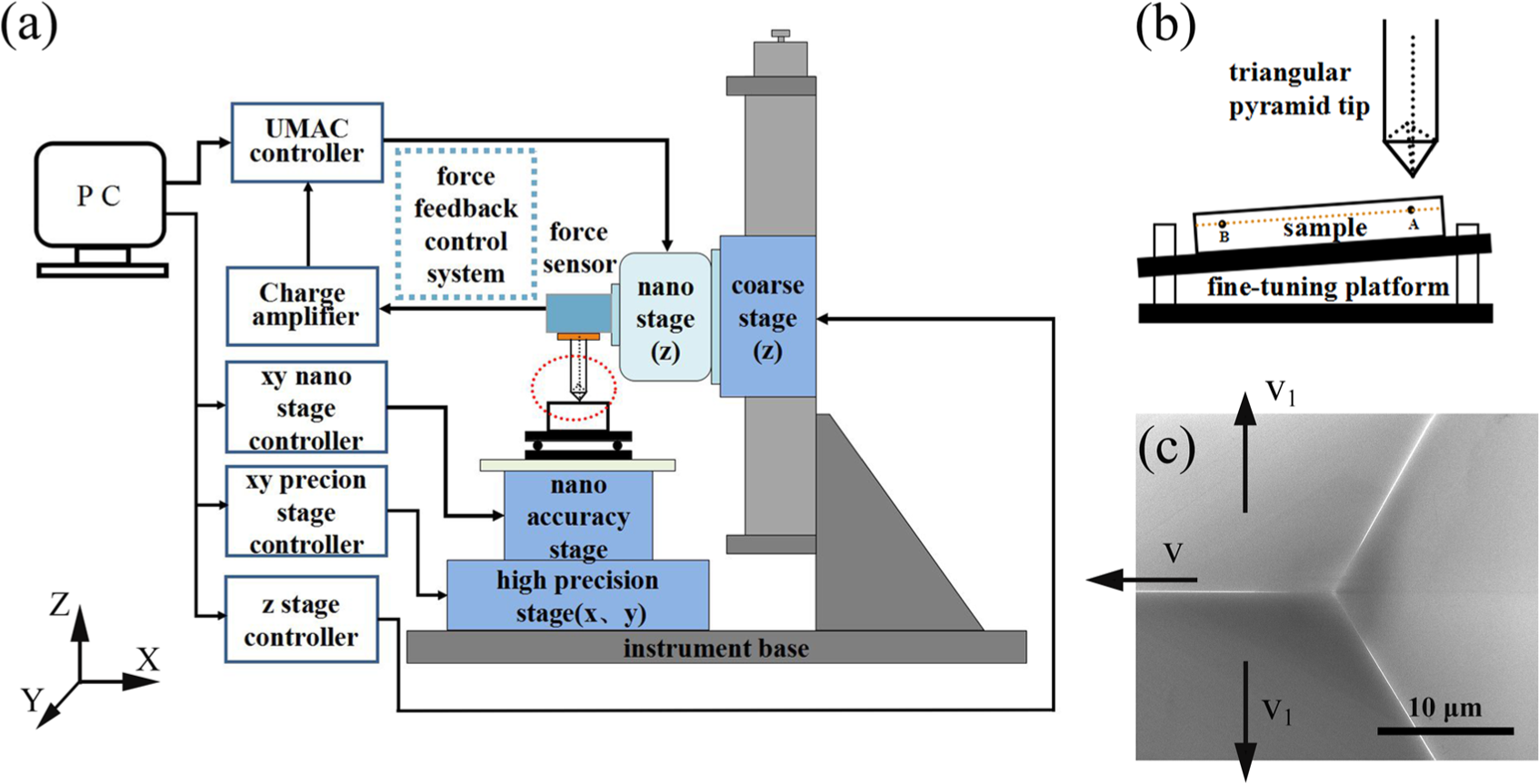
Tip-based micromachining system with force feedback control. (a) A schematic of the developed normal force-controlled tip-based micromachining system. (b) An enlarge picture of the local position of Figure (a). (c) SEM image of the cube corner tip with its shape and corresponding machining directions.

The samples used in this study are made from an aluminum alloy (2A12) that was turned using ultra-precision machine tools developed by our laboratory. The roughness (R_a) is less than 10 nm. The SEM and AFM systems used to image the machined structures are the Helios Nanolab 600i (Helios, Germany) and Dimension Icon (Bruker, Germany), respectively.

Using this system, the required normal force is set by the movement of the nanoscale accuracy stage (z) to cause the tip to penetrate the sample surface. During machining, the normal force signal is measured by the force sensor and is fed back to the UMAC through a charge amplifier. Force feedback control is used to ensure that the normal force remains almost constant by moving the nanoscale accuracy stage up and down. At this stage, there is no further need to move the coarse stage during the machining process. The coarse stage is only used to bring the tip to within 30 µm of the surface.

Response of the normal force feedback control system

Figure 2 shows a diagram of the force feedback control system. The deviation between the actual force value c(t) and the theoretical force value U(t) is represented by e(t). Integral (K_i) control is implemented to optimize the control system behavior. The K_i value is adjusted via the UMAC to ensure that the normal force remains constant during machining.

Figure 2.

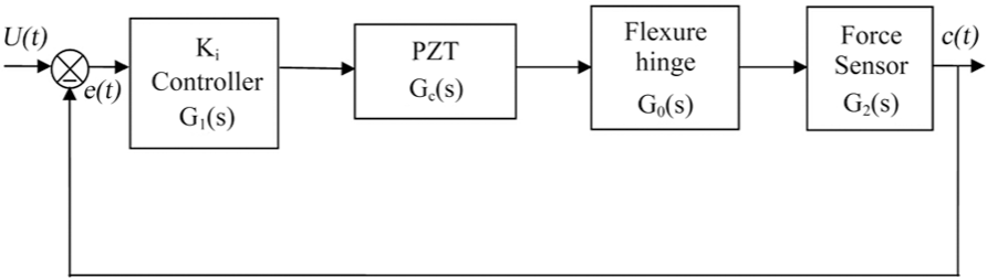
Schematic diagram of the normal force feedback control system.

The transfer function of this control system G′(s) is expressed as

G' (s) = G_{1} (s) \times G_{c} (s) \times G_{0} (s) \times G_{2} (s)

(1)

G' (s) = \frac{K_{i}}{s} \frac{K_{c}}{C R_{c} s + 1} \frac{K_{x} ω_{n}^{2}}{s^{2} + 2 ξ ω_{n} s + ω_{n}^{2}} K_{1} K_{2} = \frac{100}{s} \times \frac{3}{0.000344 s + 1} \frac{1}{0.49} \times \frac{0.75 \times {(2 π \times 983)}^{2}}{s^{2} + 2 \times 0.043 \times (2 π \times 983) s + {(2 π \times 983)}^{2}} \times 1.93

(2)

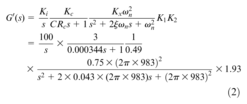
where G_c(s), G₀(s) and G₂(s) are the transfer functions of the piezoelectric ceramic (PZT), the flexure hinge of the stage and the force sensor, respectively. K₁ and K_i represent the force signal–induced changes to the voltage and integral coefficients of the control system. The time constant CR_c of the piezoelectric ceramic driving power of 0.000344 is obtained from the experimental results. K_c is determined to be 3 from the linear relationship between the input of the piezoelectric ceramic and the output of the precision stage displacement in the Z direction. The stiffness values of the piezoelectric ceramic (K_m) and the flexure hinge (K_n) are 30 and 10 N/µm, respectively. The stiffness coefficient of K_x is 0.75. A dynamic tester (Donghua Testing Technology Co., Ltd) is used to measure the frequency-domain signal using the strike method, where the average natural frequency (ω_n) of the precision stage (z) is 983 Hz and the system damping coefficient (ξ) is 0.043.

The relationship between the voltage U and the input load F is linear. The coefficient K₁ = 1/0.49. F = K₂X, which is the ideal static model characteristic equation of the sensor based on Hooke’s law. K₂ is 1.93 mN/µm for the X-displacement of the sensor.

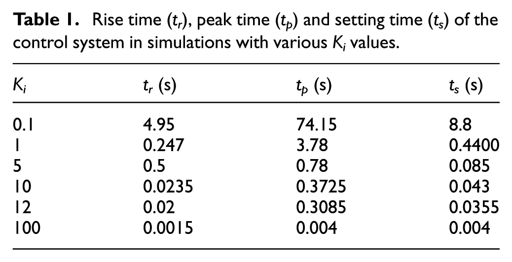
An integral link is added to the control system to ensure the system stability and reduce the system bandwidth. The coefficient K_i of the controller can be used to adjust the dynamic response of the feedback control system. The control process for this system is simulated using MATLAB software based on the model of equation (2). Figure 3(a) shows that the system has a phase margin of 72.7°, a gain margin of 2.44 dB and a cut-off frequency of 1389.5 rad/s with K_i of 100, which means that this system is stable. Figure 3(b) shows the responses to step signals with typical K_i values. Table 1 shows the corresponding control system parameters with the different K_i values. We find that with increasing K_i, the rise time (t_r), the peak time (t_p) and the setting time (t_s) all decrease. When K_i = 100, the setting time reaches 4 ms, demonstrating the good dynamic response of the system. However, when K_i exceeds 100, the control system will not be stable. In the following experiments, the K_i value of 100 is used to study the effects of the machining velocity.

Figure 3.

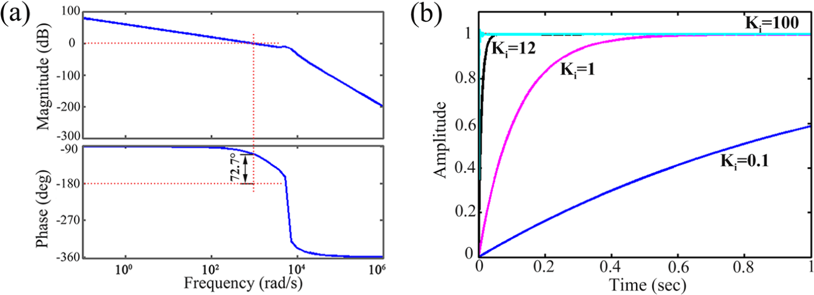
Open-loop Bode diagram and step response curve. (a) The system of Open-loop Bode diagram. (b) The response of step signals with different K_i values.

Table 1.

Rise time (t_r), peak time (t_p) and setting time (t_s) of the control system in simulations with various K_i values.

K_i	t_r (s)	t_p (s)	t_s (s)
0.1	4.95	74.15	8.8
1	0.247	3.78	0.4400
5	0.5	0.78	0.085
10	0.0235	0.3725	0.043
12	0.02	0.3085	0.0355
100	0.0015	0.004	0.004

Results and discussion

Comparison of the machining processes between the feedback control and open-loop states

Figure 4(a) and (b) shows schematics of the tip-based micromachining processes when using open-loop control and force feedback control, respectively. The original sample surface is inclined as an example. As shown in Figure 4(a), the machined surface (indicated by the dotted line) is parallel to the horizontal plane because of the motion between the tip and the sample. In Figure 4(b), the machined surface is parallel to the original surface rather than to the horizontal plane because of the feedback control of the constant normal force, and this results in the up and down motions (Δx) of the tip and the PZT.

Figure 4.

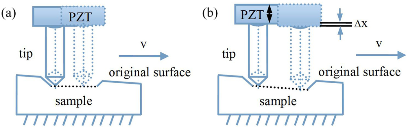
Schematic diagram of tip-based machining on an inclined surface with the normal force open-loop or closed-loop control. (a) The schematic diagram of machining with the normal force open-loop control. (b) The schematic diagram of machining with the normal force closed-loop control.

Figure 5(a) shows the variations in the normal force when scratching a single groove in the open-loop control state corresponding to Figure 4(a). The normal force is 10 mN. The machining velocity and groove length are 0.04 mm/s and 1 mm, respectively. The machining process is divided into three stages: before machining, during machining and after machining. The normal force is kept constant at 10 mN before machining, but is then gradually reduced to 1 mN during machining. In the open-loop control system, the normal force is not controlled to remain constant, as shown in Figure 4(a). The inclination of the original sample surface will thus result in variations in the normal force signal (Figure 5(a)). Figure 5(b) shows the force signal variation under the normal force feedback control condition with the same machining parameters that were used in the open-loop control state. Unlike the force signal in Figure 5(a), the normal force remains constant before, during and after the machining process. This means that the control system developed in this study can realize the required force control function.

Figure 5.

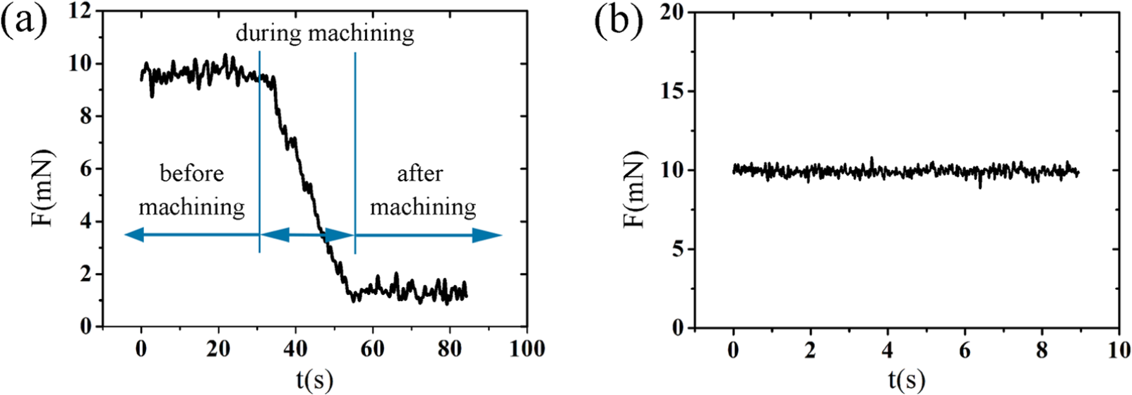
Variations in the normal forces in the open-loop and closed-loop states. (a) The normal force signal variation when scratching a single groove under the open-loop control state. (b) The normal force signal variation when scratching a single groove under the closed-loop control state.

Fabrication of single groove based on the tip-based normal force control approach

Maximum machining velocity of the normal force feedback control system

The machining velocity will influence the tip-sample state, which will in turn affect both the force control system and the machining process significantly. The machining velocity is thus very important for the force control system developed in this study. The response frequency of the control system is limited, and thus the machining velocity must have a value to which the system can respond appropriately. From the machining viewpoint, a high machining velocity leads to high machining efficiency. Therefore, the maximum machining velocity is studied in this section as follows.

Figure 6 shows the experimental response curve of the system to a step signal. When using the optimized controller parameters, the peak and setting times of this control system are 2 and 4 ms, respectively. The system overshoot is 2.4%. These results agree well with those of the theoretical analysis. Under these conditions, the normal force and the machined length of the groove are 10 mN and 1 mm, respectively. The machining velocities used are 25, 50, 100, 250, 500 and 1500 µm/s. Figure 7 shows the variations in the normal force signal with machining velocity. When the machining velocity is in the range between 25 and 250 µm/s, the constant normal force can be maintained during machining, as shown in Figure 7(a)–(d). When the machining velocity is greater than 500 µm/s, a normal force deviation is generated at the beginning of the machining process and continues with subsequent machining processes, as shown in Figure 7(e). Figure 7(f) shows that the normal force changes considerably from 8 to 12 mN when the machining velocity is increased to 1500 µm/s. Obviously, the maximum machining velocity at which the normal force can be controlled to remain constant is thus 250 µm/s in this study.

Figure 6.

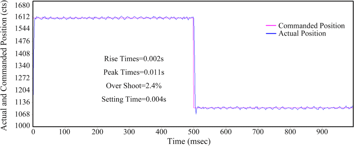
Proportional–integral–derivative system response curves (the setting time of 4 ms).

Figure 7.

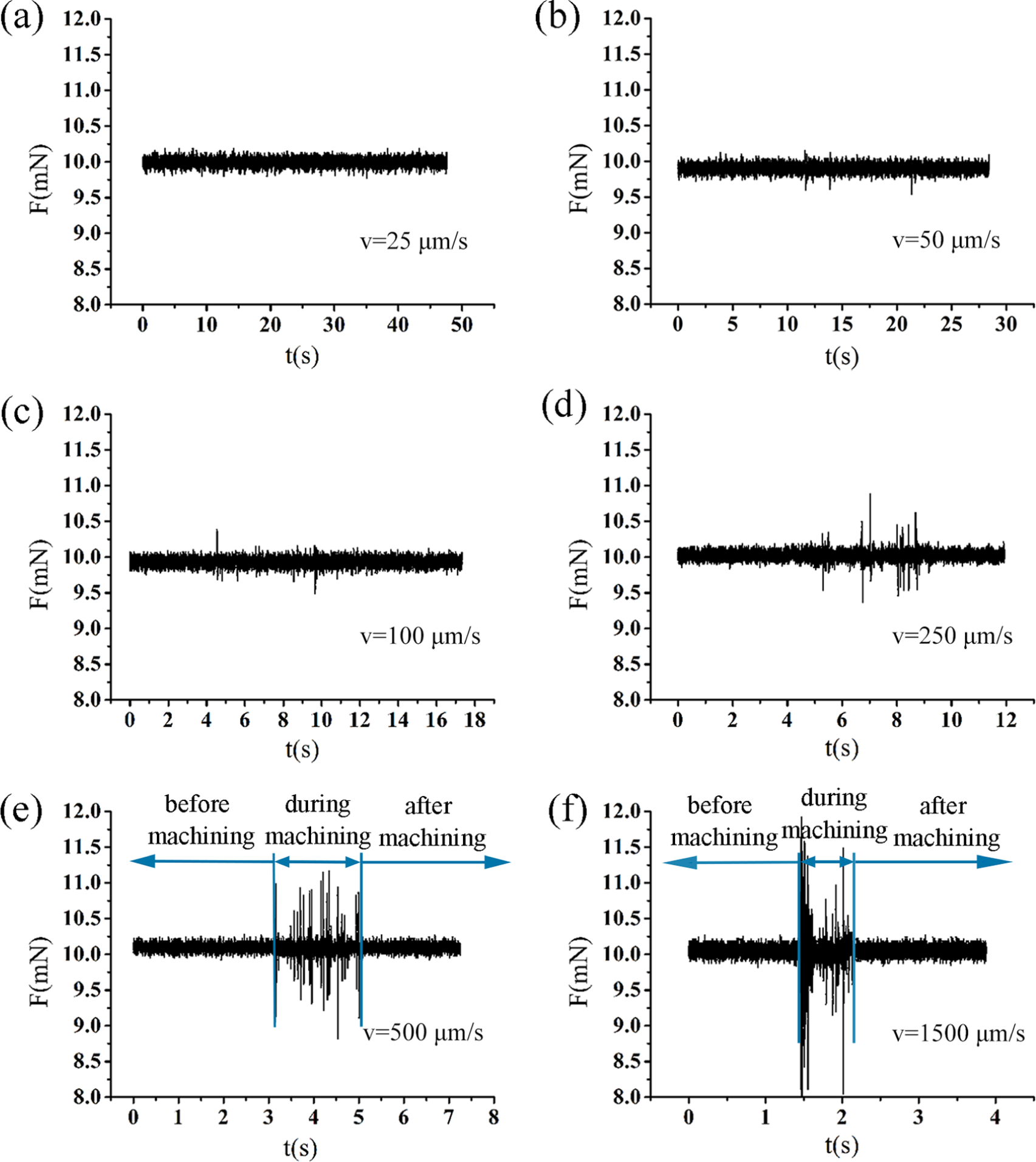
Normal force signal variation with different machining velocities. (a) The machining velocity of (a) 25 μm/s, (b)50 μm/s, (c) 100 μm/s, (d) 250 μm/s, (e) 500 μm/s, and (f) 1500 μm/s.

Prediction of groove depth for a fixed normal force

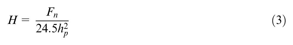
The normal force is controlled to remain constant during the machining process. Therefore, the relationship between the normal force and the machined depth must be known and is determined as follows. The Berkovich hardness $(H)$ can be expressed as a function of the applied load $(F_{n})$ and the penetration depth $(h_{p})$ in equation (3). The face angle with respect to the central axis of the indenter $(θ)$ and the projected area (A) of the cube corner tip after indentation are expressed as follows⁴⁰

H = \frac{F_{n}}{24.5 h_{p}^{2}}

(3)

A = 3 \sqrt{3} h_{p}^{2} \tan^{2} θ

(4)

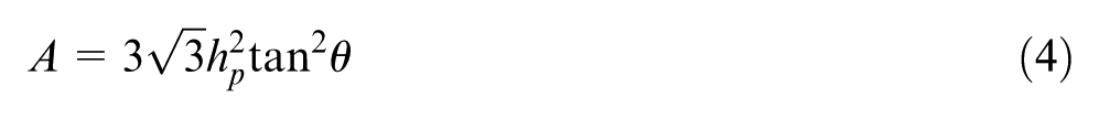
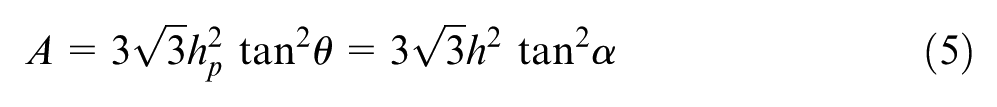
The geometry of the Berkovich indenter and the cube corner tip in this study can be determined based on the equivalent projected area, where the diamond-shaped projected area created by the Berkovich indenter is equal to the triangular pyramid contact area generated by the cube corner tip

A = 3 \sqrt{3} h_{p}^{2} \tan^{2} θ = 3 \sqrt{3} h^{2} \tan^{2} α

(5)

The groove depth h can then be obtained from equation (6) using equations (3) and (5)

h = \sqrt{\frac{F_{n}}{3 \sqrt{3} H \tan^{2} α}}

(6)

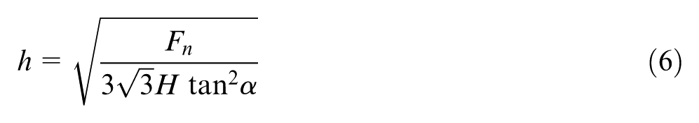
where α is 35.26° for the cube corner tip, and the aluminum alloy hardness is 2.6 GPa, as measured using a Berkovich indenter. Therefore, the relationship between the normal force and the groove depth can be obtained from equation (6) when using the cube corner tip. The relationship between the normal force and the groove depth is shown in Figure 8. The experimental and theoretical depths are indicated by the red and black lines, respectively. Groove machining tests were also carried out: the edge-forward machining direction was used and the machining velocity was 100 µm/s. The theoretical and experimental depths when the normal force is applied are presented and show only a small deviation. This shows that the theoretical model of equation (6) can be used to predict the groove depth accurately. The similar hardness equation was used to predict the width rather than the depth of the groove by Lee et al.³⁷ The reason for predicting the groove width in their studies is that the machined groove would be used as the track for the following chemical etching process. A cone tip was used to fabricate the SiO₂ film. The width of the abrasion track on SiO₂ coated silicon was from 1 to 3.5 µm with the normal force ranging from 10 to 70 mN.

Figure 8.

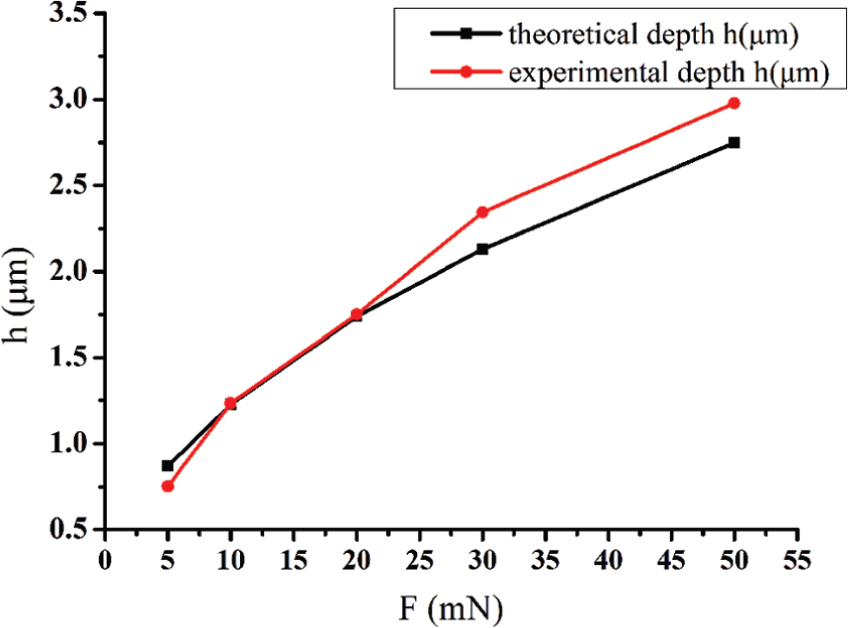
Theoretical and experimental depth variations with applied normal force.

As an example, SEM and AFM images of a groove machined with a normal force of 10 mN are presented in Figure 9. Three different positions are imaged at the front, center and rear of this groove, as shown in the SEM image of Figure 9(a). The groove depths are 1.23, 1.205 and 1.271 µm, respectively. It is thus demonstrated that the groove depth remains constant when using the normal force feedback control approach. During this test, the originally inclined sample was no need to be adjusted to level because the constant normal force can make the tip trace the sample surface. In addition, the grooves were fabricated on inclined or curved copper surfaces using a V-shaped diamond tool with the cutting angle of 90° by Herrera-Granados et al. Grooves with the depth of approximately 20 µm were machined on the copper and brass surface. The groove depth was comparable to our results. However, more complex structures are difficult to be achieved using the simple V-shaped tool.^39,41 In this work, using the cube corner tip as the cutting tool and by a complex tip trace, more complex microstructures can be machined by our setup, which will be explained in the following sections.

Figure 9.

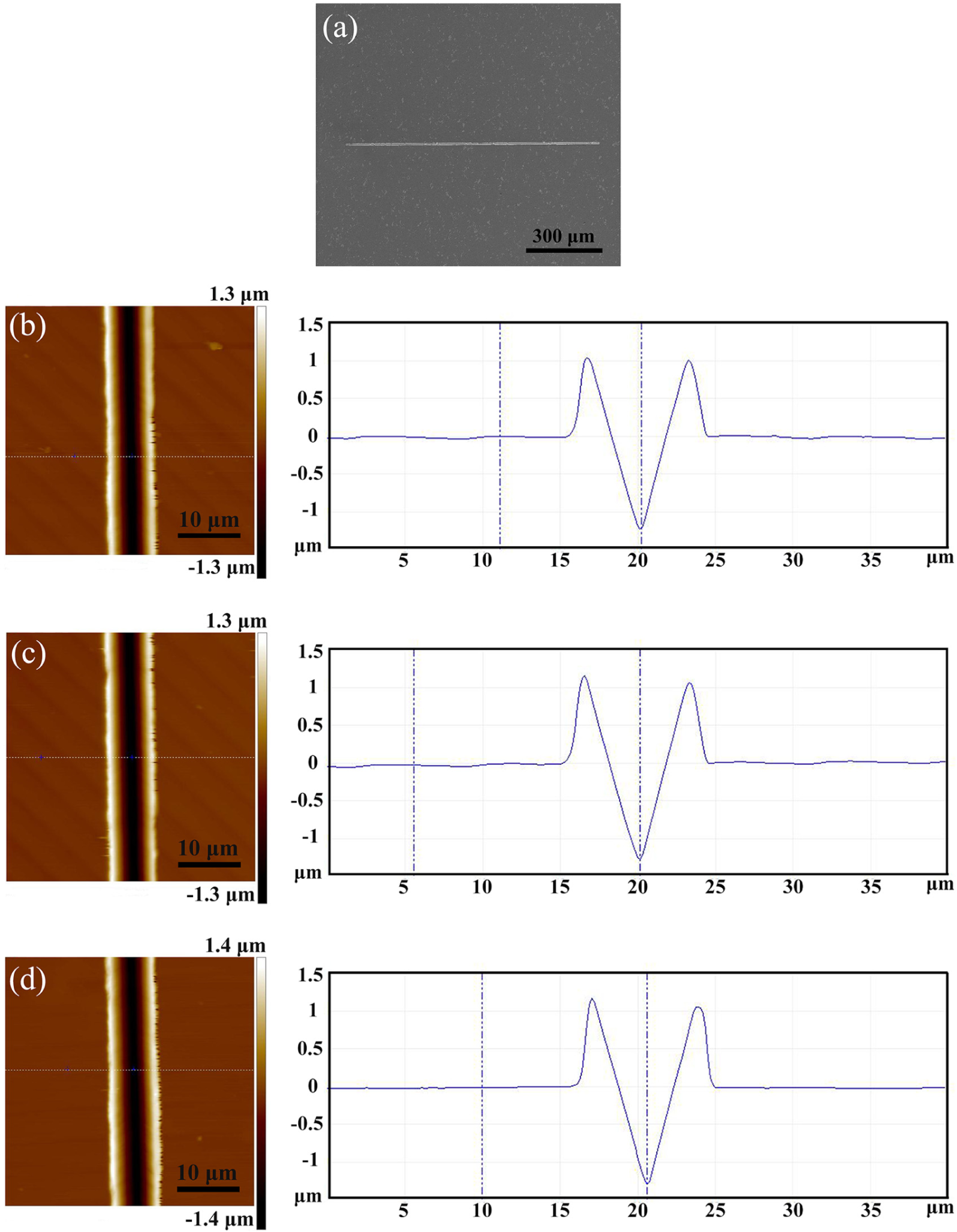
SEM image and AFM images of the grooves machined with normal force of 10 mN at various locations. (a) SEM image of the groove machined with normal force of 10 mN (b)-(d) AFM image at the front,center and rear of groove,respectively.

Fabrication of complex structures based on the tip-based normal force control approach

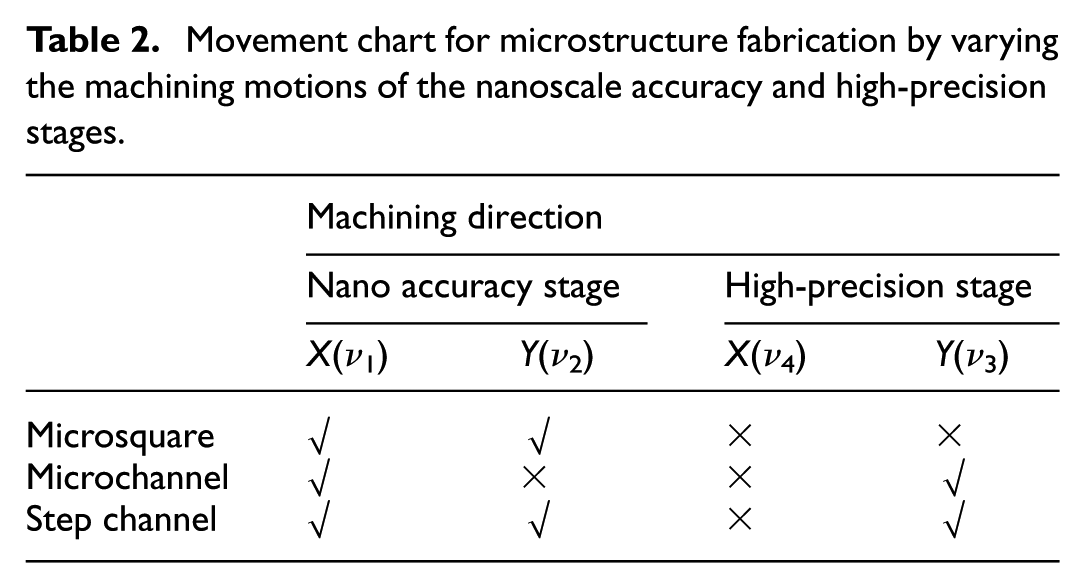
In this section, square structures and more complex structures are machined with the tip pitch using the normal force control method, demonstrating that this novel tip-based method has the potential ability to machine more complex microstructures and is likely to find wider application in the micromachining field. Figure 10 and Table 2 give the schematics and movement charts, respectively, for machining of microsquares, millimeter-scale microchannels and 3D step microchannels. These processes will be explained in detail in the following parts.

Figure 10.

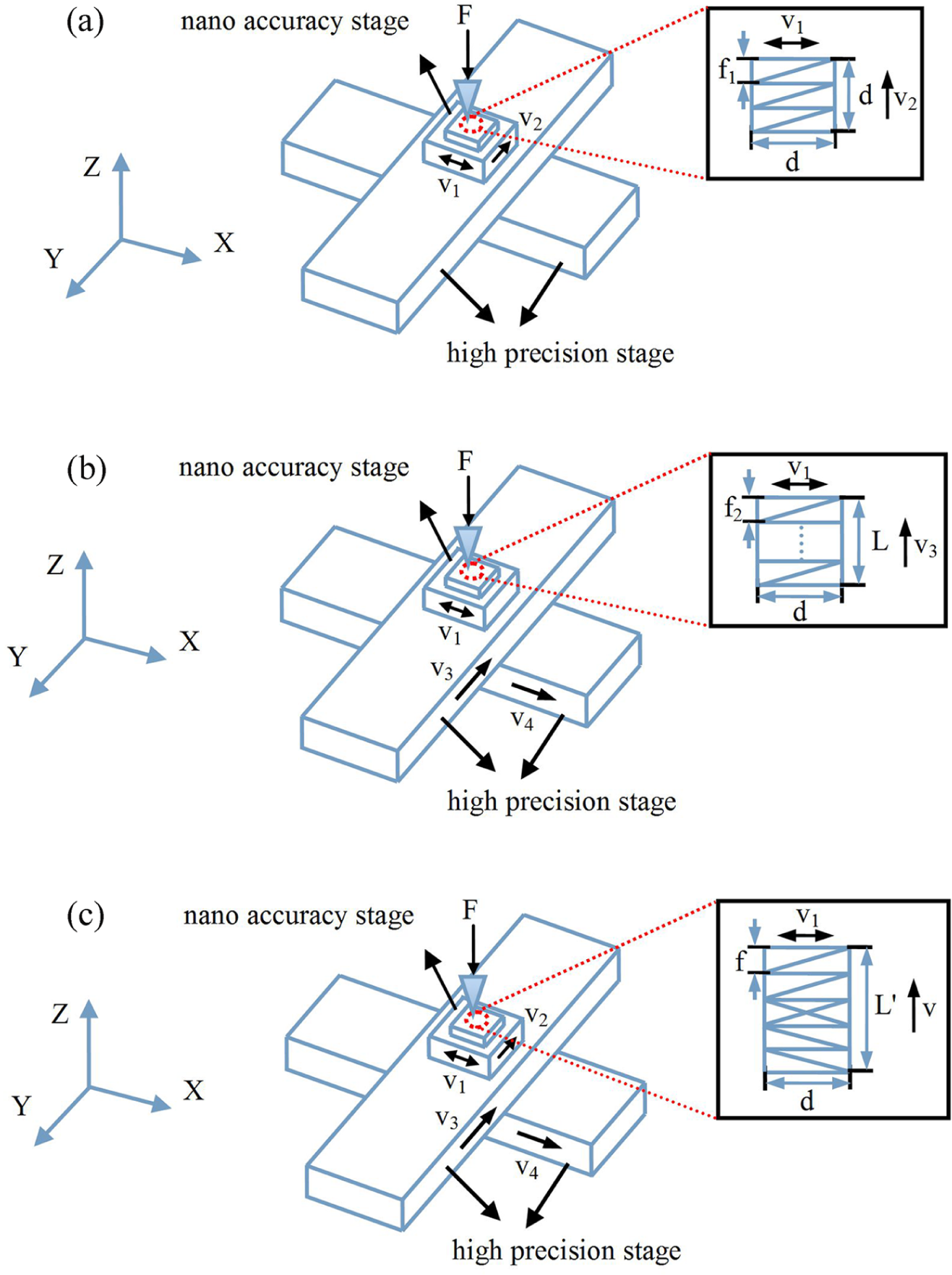
Schematic diagrams of machining processes for different microstructures with the various machining motions of the nanoscale accuracy and high-precision stages. (a) Schematic diagram of fabrication of microsquares (b) Schematic diagram of fabrication of millimeter-scale microchannels (c) Schematic diagram of fabrication of step-shaped microchannels.

Table 2.

Movement chart for microstructure fabrication by varying the machining motions of the nanoscale accuracy and high-precision stages.

	Machining direction
	Nano accuracy stage		High-precision stage
	X(ν₁)	Y(ν₂)	X(ν₄)	Y(ν₃)
Microsquare	√	√	×	×
Microchannel	√	×	×	√
Step channel	√	√	×	√

Fabrication of microsquares

The tip motion required to obtain a square structure is realized by moving the nanoscale accuracy stage in the X-Y directions, as shown in Figure 10(a). Table 2 provides the movement chart that details the changes in the machining motion of the nanoscale accuracy and high-precision stages for the single microstructure. Figure 11 shows AFM images of the square pits with a normal force of 10 mN and a machining velocity of 100 µm/s. The chosen reciprocation machining velocity (v₁) is less than the maximum machining velocity of 250 µm/s to ensure that the tip traces the sample surface with the required fixed normal force in the X direction. A feed of 800 nm is produced by moving the nanoscale accuracy stage (v₂) in the Y direction. The depth of the square pit is 3.326 µm, as shown in Figure 11(a). When the feed increases to 1000 nm, the depth of the square pit is 2.856 µm, as shown in Figure 11(b). However, when the feed reaches 1600 nm, the depth of the square pit then decreases to 2.223 µm, as shown in Figure 11(c). It is thus shown that the feed influences the machined depth when using normal force feedback control. Other researchers machined similar microsquares using the AFM-tip nanomachining method.^42–44 The depth of the squares ranges from only several nanometers to hundreds of nanometers using commercial AFM or modified commercial AFM systems. Such structures were successfully machined on the flat surface⁴² or the curved surface of a microball.^43,44 Using the AFM-tip nanomachining method, it is difficult to achieve the depth of lager than several micrometers. However, our setup can do such work using the similar normal force control principle of AFM.

Figure 11.

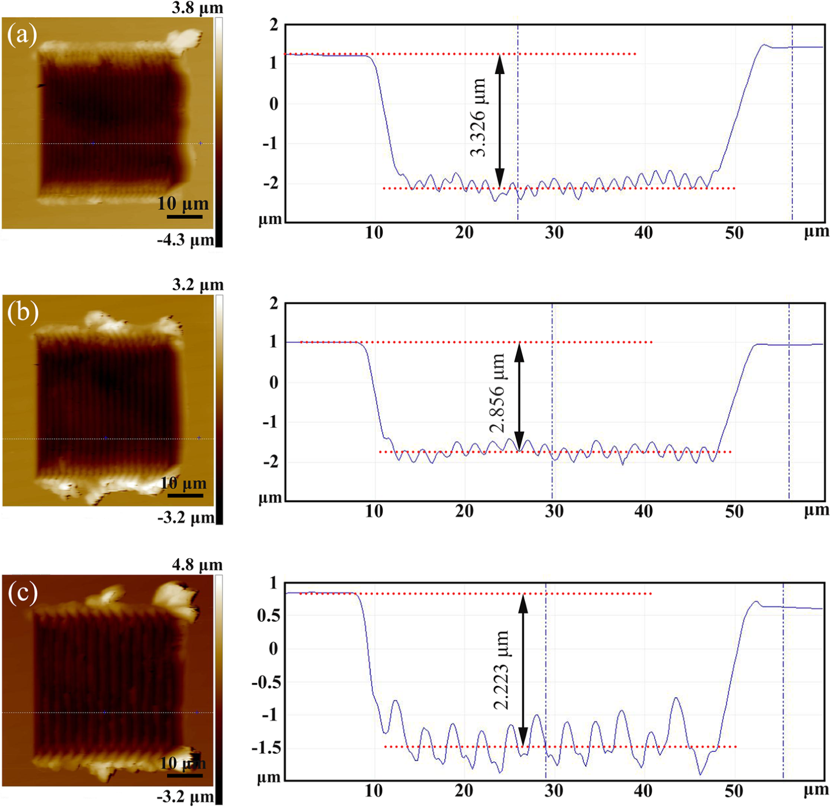
AFM images of square pits fabricated with different feeds. (a) The feed of 800 nm. (b) The feed of 1000 nm. (c) The feed of 1600 nm.

Fabrication of millimeter-scale microchannels

Figure 10(b) shows a schematic of the machining of millimeter-scale microchannels. The reciprocation motion of the tip (v₁) in the X direction is realized using the nanoscale accuracy stage. The movement length in this direction controls the width of the microchannel. The high-precision stage (v₃) is used to move both the sample and the nanoscale accuracy stage along the Y direction, thus determining the length of the microgroove. In this study, the movement range of the high-precision stage is 100 mm, which restricts the maximum channel length to 100 mm. The normal force is also 10 mN. The microchannel width is 40 µm. Under these conditions, the relationship between the velocity of the nanoscale accuracy stage in the X direction and the velocity of the high-precision stage in the Y direction determine the final machined results. The velocity (v₁) in the X direction is fixed at 100 µm/s. Machining velocities (v₃) in the Y direction of 100, 5 and 3 µm/s are used to perform the machining tests.

Figure 12(a)–(c) shows the machined results for the different machining velocities (v₃). It was found that when the machining velocity in the Y direction was 100 µm/s, rectangular microchannels cannot be formed, and only a long zigzag-shaped microgroove is formed, as shown in Figure 12(a). When the machining velocity was reduced to less than 5 µm/s in the Y direction, rectangular microchannels with suitable machined depths could be fabricated, as shown in Figure 12(b)–(d). When the machining velocity is 3 µm/s, the depth of the resulting microchannel is 2.84 µm. However, the microchannel depth is 1.95 µm when the machining velocity is 5 µm/s. A higher machining velocity thus leads to a larger feed between the tip traces. The machined depth therefore decreases with increasing machining velocity. This is similar to the behavior observed when machining square pits, as shown in Figure 11.

Figure 12.

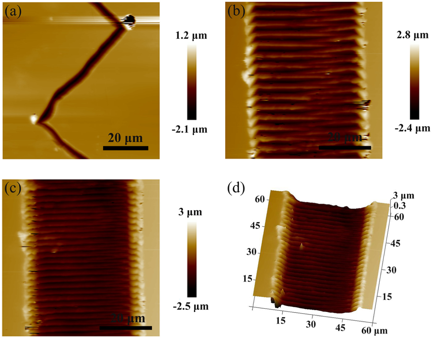
AFM images of machining processes for rectangular microchannels with various machining velocities. (a) The machining velocity of 100 μm/s in the Y direction. (b) The machining velocity of 5 μm/s in the Y direction. (c) The machining velocity of 3 μm/s in the Y direction. (d) Three-dimensional view of structures with the machining velocity of 3 μm/s.

Figure 13(a) and (b) shows the overall and enlarged SEM images of a microchannel array that was produced by moving the high-precision stage in the Y direction (v₄). The machining velocity in the Y direction is 5 µm/s. The microchannel length is 1 mm, and the pitch between two adjacent microchannels is 20 µm.

Figure 13.

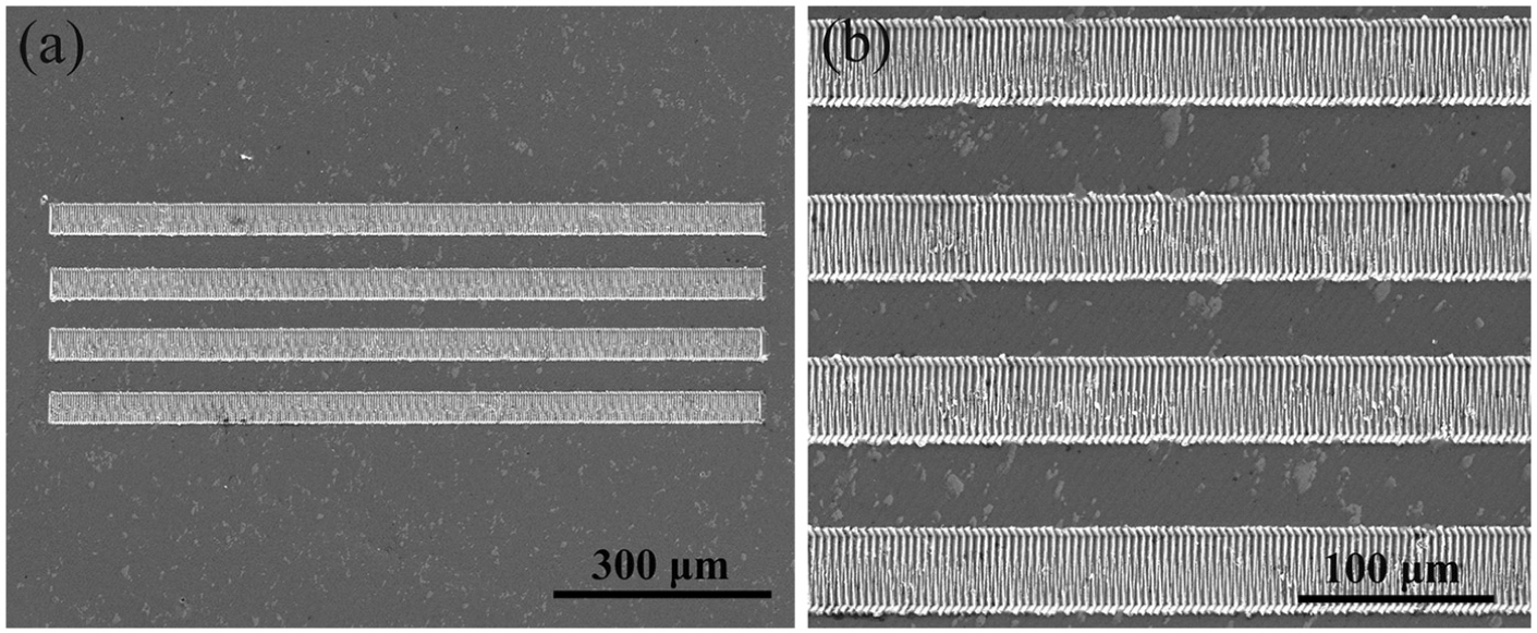
SEM images of a wide range of array rectangular microchannel arrays. (a) The overall SEM image of rectangular microchannel arrays. (b) The enlarged SEM image of rectangular microchannel arrays.

Fabrication of 3D step microchannels

More complex microstructures with micrometer machined depths can be fabricated using the normal force feedback control method. Figure 10(c) shows a schematic of a step microstructure machining process based on integrated movement of the nanoscale accuracy stage and the high-precision stage. The nanoscale accuracy stage moves in the X and Y directions with a specified pitch. If the high-precision stage does not move, the machined structure is a square pit, similar to that shown in Figure 11. However, if the high-precision stage moves simultaneously and continuously along the Y direction, the machined squares will overlap. Because the normal force is controlled to be constant, the depth at the overlap position will be deeper than at a non-overlapped position. Increasing numbers of overlaps will lead to deeper machined channels, as shown in Figure 10(c).

The reciprocation machining velocity (v₁) in the X direction is 100 µm/s slower than the maximum machining velocity of the normal force feedback control system. The feed length is 400 nm. The machining velocity in the Y direction is 0.4 µm/s. The width of the square (d) is 40 µm. Figures 14 and 15 show AFM and SEM images of the machined step structures, respectively. The depths of the step-shaped microchannel shown in Figure 14(a) are 3.65 and 7.46 µm. Figure 14(b) shows one half of a step microchannel with four different depths that was fabricated using different numbers of overlaps. The depths of the four steps are 2.14, 3.425, 5.167 and 5.6 µm. Figure 15 shows the SEM images of a wide range of step-shaped microchannels fabricated using different numbers of cycles. The numbers of cycles in Figure 15(a)–(c) are 10, 5 and 3, respectively.

Figure 14.

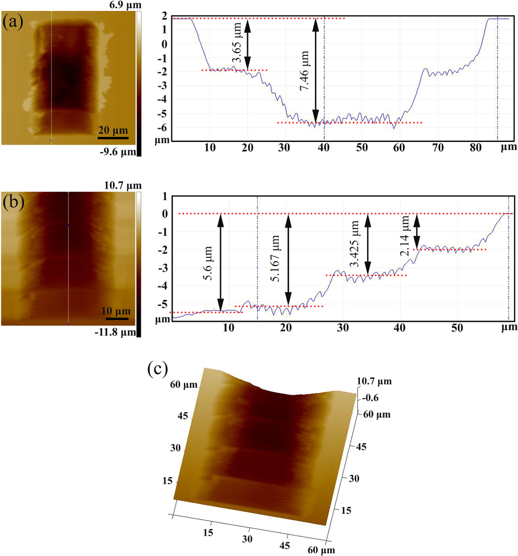
AFM images of the step-shaped microchannels. (a) The machining velocity of 0.4 μm/s with the number cycle of 2. (b) One half of a step-shaped microchannel with four different depths. (c) Three-dimensional one half of a step-shaped microchannel.

Figure 15.

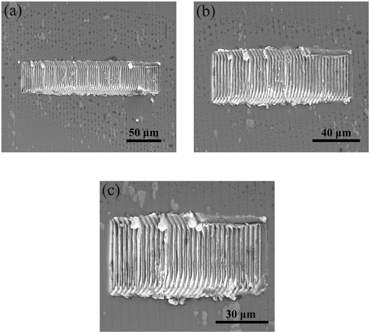
SEM images of step-shaped microchannels fabricated using different numbers of cycles. (a) SEM images of step-shaped microchannels with the number of cycle of 10. (b) The number of cycle of 5. (c) The number of cycle of 3.

Conclusion

In this study, a tip-based micromachining device using the normal force control method similar to the conventional AFM system is first established. The stability and the dynamic response of the control system of this device are studied. An integral link is added to the control system to guarantee the system stability and reduce the system bandwidth. When setting time of the control system is 4 ms, the maximum machining velocity that can be obtained for our system is 250 µm/s to keep the normal force constant during machining. In addition, a model for predicting the machined depth with the known normal force is presented.

By controlling the X-Y nanoscale accuracy stage and the X-Y high-precision stage of this system to realize the complex movements of the tip, microsquares, millimeter-scale microchannels and 3D step microchannels are successfully fabricated using the normal force control method. Using the movements of the X-Y nanoscale accuracy stage, the depths of 40 µm × 40 µm microsquares range from 2 to 3.5 µm with the machining feeds from 800 to 1600 nm and the constant normal force of 10 mN. With only one reciprocation direction motion of the nano accuracy stage and the one direction motion of the high-precision stage, the microchannels with 1 mm in length and 40 µm in width are machined. Combination of duplicated scans in two directions of the nanoscale accuracy stage and the one direction movement of the high-precision stage can lead to different numbers of overlaps of the machined area. Thus, the step microchannels with different depths can be fabricated with a constant normal force.

Many researchers have already been aware of the merit of the normal force control micromachining method. Based on this work, the complex microstructures machined by this way could be applied in different research fields, such as solar cell, chemical material transport and microchip cooling in the future. And the force control method has the property of tracing the sample surface, like AFM, thus this method will be extended to fabricate micro/nanostructures on inclined or curved surfaces.

Footnotes

Appendix 1 Declaration of conflicting interests

The author(s) declared no potential conflicts of interest with respect to the research, authorship and/or publication of this article.

Funding

The author(s) disclosed receipt of the following financial support for the research, authorship, and/or publication of this article: This work was financially supported by the National Natural Science Foundation of China (Grant Nos. 51521003 and 51675134), Self-Planned Task (SKLRS201606B) of State Key Laboratory of Robotics and System (HIT) and the National Program for Support of Top-notch Young Professors.

References

Savu

Silveira

Flacker

et al . Micro-reactors for characterization of nanostructure-based sensors. Rev Sci Instrum 2012; 83(5): 055104.

Hedrick

Brown

Kluender

et al . Hard transparent arrays for polymer pen lithography. ACS Nano 2016; 10(3): 3144–3148.

Rathod

Doloi

Bhattacharyya

. Experimental investigations into machining accuracy and surface roughness of microgrooves fabricated by electrochemical micromachining. Proc IMechE, Part B: J Engineering Manufacture 2015; 229(10): 1781–1802.

Malshe

Rajurkar

Virwani

et al . Tip-based nanomanufacturing by electrical, chemical, mechanical and thermal processes. CIRP Ann: Manuf Techn 2010; 59(2): 628–651.

Huo

Cheng

. A dynamics-driven approach to the design of precision machine tools for micro-manufacturing and its implementation perspectives. Proc IMechE, Part B: J Engineering Manufacture 2008; 222: 1–13.

Lee

Yeoh

Timchenko

et al . Heat transfer enhancement in micro-channel with multiple synthetic jets. Appl Therm Eng 2012; 48: 275–288.

Van Lerberghe

Motsegood

et al . Three-dimensional micro-channel fabrication in polydimethylsiloxane (PDMS) elastomer. J Microelectromech S 2000; 9(1): 76–81.

González-Campo

Eker

Gardeniers

et al . A supramolecular approach to enzyme immobilization in micro-channels. Small 2012; 8(22): 3531–3537.

Liu

Zhang

Dong

et al . Fabrication of silicon nanopillar arrays by cesium chloride self-assembly and wet electrochemical etching for solar cell. Appl Surf Sci 2014; 289: 300–305.

10.

Zheng

Wang

Jiang

et al . Research status and application prospects of manufacturing technology for micro-nano surface structures with low reflectivity. Proc IMechE, Part B: J Engineering Manufacture 2015; 229(11): 1877–1892.

11.

Wolden

Kurtin

Baxter

et al . Photovoltaic manufacturing: present status, future prospects, and research needs. J Vac Sci Technol A 2011; 29(3): 030801.

12.

Dongre

Vesvikar

Singh

et al . Modeling of silicon ingot slicing process by wire-electrical discharge machining. Proc IMechE, Part B: J Engineering Manufacture 2013; 227(11): 1664–1678.

13.

Ferchichi

Laariedh

Sow

et al . Fabrication of disposable flexible SERS substrates by nanoimprint. Microelectron Eng 2015; 140: 52–55.

14.

Siitonen

Kontturi

et al . Disposable gold coated pyramidal SERS sensor on the plastic platform. Opt Express 2016; 24(1): 724–731.

15.

Lin

Stuparu

Huntington

et al . Nanopatterned substrates increase surface sensitivity for real-time biosensing. J Phys Chem C 2013; 117(10): 5286–5292.

16.

Zhu

Bai

et al . Reusable three-dimensional nanostructured substrates for surface-enhanced Raman scattering. Nanoscale Res Lett 2014; 9(1): 1–8.

17.

Tang

Wei

. Fabrication of anisotropic metal nanostructures using innovations in template-assisted lithography. ACS Nano 2012; 6(2): 998–1003.

18.

Sun

Luo

Ritchie

et al . A predictive divergence compensation approach for the fabrication of three-dimensional microstructures using focused ion beam machining. Proc IMechE, Part B: J Engineering Manufacture 2012; 226(2): 229–238.

19.

Gao

Fang

et al . High performance surface-enhanced Raman scattering substrates of Si-based Au film developed by focused ion beam nanofabrication. Nanoscale Res Lett 2012; 7(1): 1–8.

20.

Ahmed

Darwish

Alahmari

. Laser ablation and laser-hybrid ablation processes: a review. Mater Manuf Process 2016; 31(9): 1121–1142.

21.

Richards

Baker

Wilson

et al . Femtosecond laser ablation of cadmium tungstate for scintillator arrays. Opt Laser Eng 2016; 83: 116–125.

22.

Zou

et al . Influence of porous structure on the machining performance of micro EDM. J Mater Process Tech 2016; 232: 43–51.

23.

Wang

Yang

Qian

et al . Study of alternating current flow in micro-EDM through real-time pulse counting. J Mater Process Tech 2016; 231: 179–188.

24.

Wang

Hong

Zeng

et al . AFM tip hammering nanolithography. Small 2009; 5(4): 477–483.

25.

Chen

Hsu

Lin

. Fabrication of metal nanowires by atomic force microscopy nanoscratching and lift-off process. Nanotechnology 2005; 16(8): 1112–1115.

26.

Tseng

Shirakashi

Nishimura

et al . Scratching properties of nickel-iron thin film and silicon using atomic force microscopy. J Appl Phys 2009; 106(4): 044314.

27.

Sumomogi

Endo

Kuwahara

et al . Micromachining of metal surfaces by scanning probe microscope. J Vac Sci Technol B 1994; 12(3): 1876–1880.

28.

Brousseau

Krohs

Caillaud

et al . Development of a novel process chain based on atomic force microscopy scratching for small and medium series production of polymer nanostructured components. J Manuf Sci E-T ASME 2010; 132(3): 030901.

29.

Yan

Zhao

et al . Top-down nanomechanical machining of three-dimensional nanostructures by atomic force microscopy. Small 2010; 6(6): 724–728.

30.

Wang

Jiao

et al . Nanochannel system fabricated by MEMS microfabrication and atomic force microscopy. IET Nanobiotechnol 2011; 5(4): 108–113.

31.

Oliver

Pharr

. An improved technique for determining hardness and elastic modulus using load and displacement sensing indentation experiments. J Mater Res 1992; 7(6): 1564–1583.

32.

Huang

Hsieh

Wang

et al . Investigation of scratching nano grooves on aluminum film. In: Proceedings of the 2009 IEEE international conference on nano/molecular medicine and engineering (NANOMED), Tainan, Taiwan, 18–21 October 2009, pp.146–149. New York: IEEE.

33.

Adams

Allan

Briscoe

et al . An experimental study of the nano-scratch behaviour of poly (methyl methacrylate). Wear 2001; 251(1): 1579–1583.

34.

Youn

Kang

. Maskless pattern fabrication on Si (100) surface by using nanoindenter with KOH wet etching. Scripta Mater 2004; 50(1): 105–109.

35.

Youn

Kang

. Effect of nanoscratch conditions on both deformation behavior and wet-etching characteristics of silicon (100) surface. Wear 2006; 261(3): 328–337.

36.

Gao

Lee

Noh

et al . In-process micro/nano measurement for micro cutting. In: Cheng

Huo

(eds) Micro-cutting: fundamentals and applications. London: John Wiley & Sons, 2013, pp.315–344.

37.

Lee

Jin

Kim

. Application of single asperity abrasion process for surface micro-machining. Wear 2001; 251(1): 1133–1143.

38.

Herrera-Granados

Ashida

Ogura

et al . Basic study on micro/nano scale cutting applying machining force control system. In: JSPE Semestrial Meeting, 12–14 September 2013, Osaka, Japan, pp. 319–320.

39.

Herrera-Granados

Ashida

Ogura

et al . Effect of cutting angles during the micro-groove fabrication process using a non-rigid cutting mechanism. In: Proceedings of the 9th international workshop on microfactories (IWMF)

5–8 October 2014

Honolulu, Hawaii, USA, pp. 108–115.

40.

Fischer-Cripps

Mustafaev

. Introduction to contact mechanics. New York: Springer, 2000.

41.

Herrera-Granados

Morita

Hidai

et al . Development of a non-rigid micro-scale cutting mechanism applying a normal cutting force control system. Precis Eng 2016; 43: 544–553.

42.

Geng

Yan

Zhao

et al . Fabrication of millimeter scale nanochannels using the AFM tip-based nanomachining method. Appl Surf Sci 2013; 266: 386–394.

43.

Yan

Sun

Zhao

et al . Fabrication of microstructures on the surface of a micro/hollow target ball by AFM. J Micromech Microeng 2008; 18(3): 035002.

44.

Zhao

Geng

et al . Fabrication and measurement of nanostructures on the micro ball surface using a modified atomic force microscope. Rev Sci Instrum 2012; 83(11): 115104.

Study of the control process and fabrication of microstructures using a tip-based force control system

Abstract

Keywords

Introduction

Experimental setup and details

Response of the normal force feedback control system

Results and discussion

Comparison of the machining processes between the feedback control and open-loop states

Fabrication of single groove based on the tip-based normal force control approach

Maximum machining velocity of the normal force feedback control system

Prediction of groove depth for a fixed normal force

Fabrication of complex structures based on the tip-based normal force control approach

Fabrication of microsquares

Fabrication of millimeter-scale microchannels

Fabrication of 3D step microchannels

Conclusion

Footnotes

Appendix 1

Declaration of conflicting interests

Funding

References