Sage Journals: Discover world-class research

Abstract

Disassembly levelling is to determine disassembly structures that specify components to be obtained from end-of-use/life products, and disassembly lot-sizing is to determine the timing and quantity of disassembling end-of-use/life products to satisfy the demands of their components. As an extension of the previous studies that consider them separately, this study integrates the two problems, especially in the form of multi-period model. Particularly, this study considers a generalized integrated problem in which disassembly levels may be different for the products of the same type. To describe the problem mathematically, we develop an integer programming model that minimizes the sum of setup, operation and inventory holding costs. Then, due to the problem complexity, a heuristic algorithm is proposed that consists of two phases: (a) constructing an initial solution using a priority-based greedy heuristic and (b) improving it by removing unnecessary disassembly operations after characterizing the properties of the problem. To show the performance of the heuristic algorithm, computational experiments were performed on various test instances and the results are reported.

Keywords

Disassembly levelling disassembly lot-sizing multi-period model integer programming heuristic

Introduction

Excessive consumptions of natural resources and other environmental deteriorations reveal that something is wrong with the earth, which gave rise to a new philosophical concept for our society and environment, called the sustainability. In general, sustainability can be described as the capacity for continuation into the future. Despite its vagueness and ambiguity, the concept of sustainability became a fundamental background in developing an integrated view on the earth’s future. In summary, we have to provide sustainable economy and environment for the next generation. See Mebratu¹ and Robèrt et al.² for more details on the concept of sustainability.

Treating end-of-use/life products is one of the major issues for sustainable society and environment, mainly due to (a) rapid development of products, (b) shortened product lives, (c) shortages of dumping and incineration sites and (d) legislation pressures to protect the environment – in particular, the legislation pressures imposed on manufacturing/service firms to collect, reuse, remanufacture, recycle and even dispose of end-of-use/life products in an environmentally conscious way; for example, see eco-design requirements for energy using products (EuP), waste electrical and electronic equipment (WEEE), restriction on the use of certain hazardous substance (RoHS) in electric and electronic equipment, and directives for end-of-life vehicles (ELV). Moreover, consumers recognize the opportunities for purchasing environmental conscious products.

Reverse logistics, which is an opposite direction of the conventional forward logistics, is a process-based framework for dealing with end-of-use/life products. In general, reverse logistics is defined as the logistics activities all the way from end-of-use/life products no longer required by users to products again usable in a market or disposable in the environmentally conscious way.^3–8 Reverse logistics, whose main activities include collection, disassembly, sorting/test, recovery (repair, reuse, recycling and remanufacturing), disposal, etc., aims at planning and executing the activities associated with end-of-use/life products effectively and efficiently. Figure 1 shows the bi-directional logistics that consists of forward and reverse logistics.⁶

Figure 1.

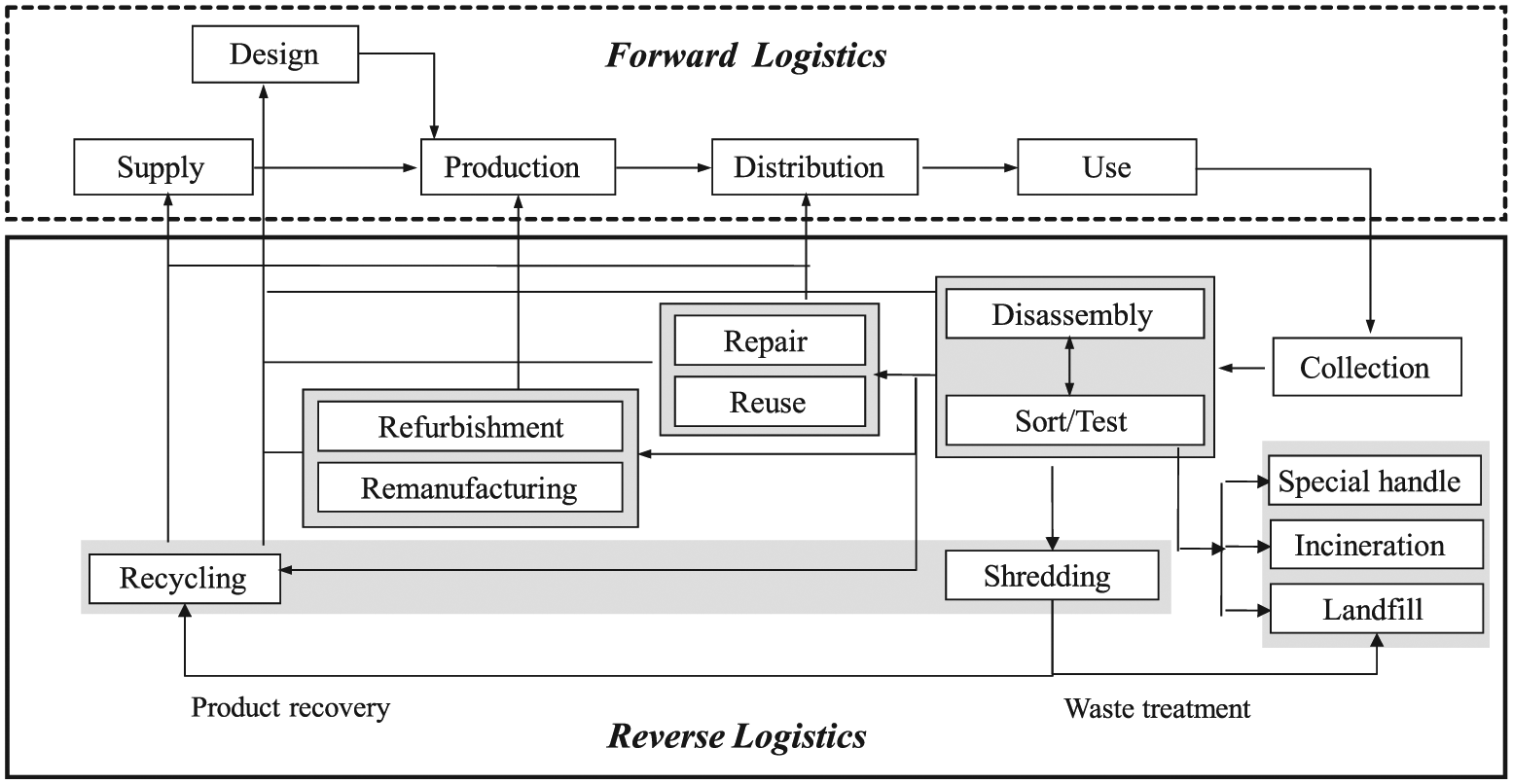
Forward and reverse logistics.

This study focuses on disassembly, one of the indispensable activities for recovering and disposing of products in reverse logistics. In general, disassembly is defined as the systematic separation of an assembly into its components or other groupings. In other words, it separates a product into its parts and/or subassemblies for the purposes of recovering materials, isolating hazardous substances, separating reusable parts/subassemblies and so on. Note that disassembly is one of the important domains in reverse logistics since end-of-use/life products cannot be recovered or even disposed of without disassembling them. The decision problems on disassembly systems include design for disassembly, disassembly line balancing, disassembly process planning, disassembly lot-sizing and so on. For more details on the disassembly problems, see Jovane et al.,⁹ Gungor and Gupta¹⁰ and Lee et al.¹¹

Among the disassembly problems mentioned earlier, we focus on disassembly levelling and lot-sizing. For a given end-of-use/life product, disassembly levelling is the problem of determining its disassembly structure that specifies components to be obtained. Note that disassembly levelling is one of the disassembly process planning activities that prepare detailed disassembly operation instructions. Also, disassembly lot-sizing, alternatively called disassembly scheduling in the literature, specifies the quantity and timing of disassembling the product in order to satisfy the demands of their components.

As in other process and production planning problems, disassembly levelling and lot-sizing have a strong relationship in that the disassemble level of a product is one of the basic input data required for disassembly lot-sizing that satisfies the demands of components specified by the corresponding disassemble structure. If the two problems are considered separately, the final solution may be local optimum or even infeasible. See Lee et al.¹¹ and Kim et al.¹² for the importance of integrating disassembly process planning and lot-sizing. In addition, the existing separated approaches have a fundamental weakness that disassembly levels must be fixed for each product type. Instead, this study considers a generalized case that allows different disassembly levels even for products of the same type, and hence more efficient solutions can be obtained that optimize a given performance measure associated with disassembly processes.

To the best of the authors’ knowledge, the only previous one that considers disassembly levelling and lot-sizing at the same time is Kang et al.¹³ who suggest a single-period model. See the next section for the literature review. As an extension of the existing single-period model, this study considers a multi-period one for the purpose of considering dynamic component demands over a planning horizon, especially multiple product types with parts commonality, that is, different product types may share their components. Although the parts commonality can reduce disassembly costs by avoiding unnecessary disassembly operations, it makes the problem much more complicated.¹²

To represent the multi-period disassembly levelling and lot-sizing problem mathematically, an integer programming model is suggested for the objective of minimizing the sum of setup, operation and inventory holding costs. Then, due to the problem complexity, we suggest a two-phase heuristic that consists of constructing an initial solution and improvement. The initial solution is obtained using a priority-based greedy heuristic, and then it is improved by eliminating the unnecessary disassembly operations after characterizing the problem properties. To test the heuristic algorithm, computational experiments were done on various instances, and the results are reported.

The article is organized as follows. In the next section, we review the previous studies on disassembly process planning and lot-sizing. The third section describes the problem in more detail with an integer programming model. The two-phase heuristic and its test results are presented in the fourth and fifth sections, respectively. Finally, the last section concludes the article with a summary and discussion of future research areas.

Literature review

This section reviews the previous studies on disassembly process planning and lot-sizing. The review consists of three parts: (a) disassembly process planning, (b) disassembly lot-sizing and (c) integrated disassembly process planning and lot-sizing.

Disassembly process planning

There are a number of previous studies on disassembly process planning, which can be classified according to the three main decision variables: (a) disassembly level – whether additional disassembly operations are performed or not at each stage of disassembling a product; (b) disassembly sequence – sequence of disassembly operations; and (c) end-of-life options – how each part or subassembly is to be treated, for example, reuse, remanufacturing, recycling, disposal and so on. See O’Shea et al.,¹⁴ Lee et al.,¹¹ Santoch et al.¹⁵ and Lambert¹⁶ for literature reviews on disassembly process planning.

Most of the earlier studies consider only one decision variable, for example, Penev and De Ron¹⁷ and Igarashi et al.¹⁸ for disassembly levelling; Lambert,¹⁹ Hui et al.,²⁰ Adenso-Diaz et al.²¹ and Jin et al.²² for disassembly sequencing; and Bufardi et al.²³ and Jun et al.²⁴ for determining end-of-life options. As an extension, several articles consider two decision variables at the same time; for example, see Pnueli and Zussman,²⁵ Johnson and Wang,^26,27 Lambert,^28,29 Kang et al.^30,31 and Vinodh et al.^32,33 for determining disassembly level and sequence at the same time. Finally, some other articles consider all the three decision variables, for example, see Erdos et al.,³⁴ Teunter,³⁵ Behdad et al.³⁶ and Ma et al.³⁷

Disassembly lot-sizing

As a mid- or short-term planning activity, various researches have been done on disassembly lot-sizing. According to the review of Kim et al.,¹² the previous studies can be classified according to the number of product types (single and multiple product types) and the product structure (assembly structure without parts commonality and general structure with parts commonality). See Lee et al.³⁸ for the mathematical model for each of the problem classes.

Most of the earlier studies consider the basic problem, that is, a single assembly structured product without parts commonality. Gupta and Taleb³⁹ suggest a material requirement planning (MRP) like algorithm without an explicit objective function. Lee and Xirouchakis⁴⁰ suggest a heuristic algorithm for the problem with a cost-based objective and later, Kim et al.⁴¹ suggest an optimal algorithm after proving that the cost-based problem is non-deterministic polynomial (NP)-hard. For the capacitated version of the basic problem, see Lee et al.,⁴² Jeon et al.⁴³ and Kim et al.⁴⁴ As an extension of the basic problem, other articles consider the problem with parts commonality. For example, see Taleb et al.⁴⁵ for a single product type and Taleb and Gupta,⁴⁶ Lambert and Gupta,⁴⁷ Kim et al.^48,49 and Langella⁵⁰ for multiple product types.

Disassembly process planning and lot-sizing

To deal with the fact that disassembly process planning and lot-sizing are highly interdependent, several articles tried to integrate the two problems by considering different decision variables of each problem.

Most research articles consider the disassembly lot-sizing problem with an additional decision on end-of-life options such as reuse, remanufacturing, recycling and disposal. Veerakamolmal and Gupta⁵¹ consider the problem of determining the number and types of products to disassemble and dispose of in order to satisfy the demands of required parts, and suggest an algorithm that maximizes the profit, and later, Kongar and Gupta⁵² extend the earlier one by suggesting a fuzzy goal programming model for the multi-criteria problem that determines the number of products to be collected and the number of parts to be reused, recycled, stored, and disposed of in stochastic disassemble-to-order systems. Xanthopoulos and Iakovou⁵³ suggest a simulation-based solution approach for the problem of selecting subassemblies to disassemble and determining the number of products to be collected, disassembled, recycled, remanufactured and disposed of. Finally, as explained earlier, Kang et al.,¹³ the only previous study on disassembly levelling and lot-sizing at the same time, suggest an optimal polynomial algorithm for the basic single-period disassembly levelling and lot-sizing problem and a heuristic algorithm for an extension with parts commonality after proving its NP-hardness.

Problem description

Before describing the problem, the disassembly structure for multiple product types with parts commonality is explained with the disassembly bill of material (d-BOM). In the d-BOM structure, the root items represent the products to be disassembled and the leaf items are components that cannot be disassembled further. A parent item is an item that has at least one child item and a child item is an item that has at least one parent. The parts commonality, that is, product or subassembly shares its components, is represented in that a component has two or more parent items. Figure 2 shows an example of the d-BOM structure with two product types. In this example, 1 and 2 are root items and 7, 8, 9 and 10 are leaf items. Also, item 8 (9), represented as a bolded box, is a common item since it has two parents 3 (4) and 4 (5). The number in parentheses represents the number of the item that can be obtained from disassembling its parent, that is, yield.

Figure 2.

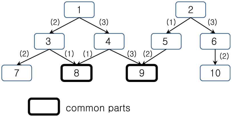
d-BOM structure for multiple product types with parts commonality: example.

Now, the multi-period disassembly levelling and lot-sizing problem considered in this study can be defined as the problem of determining the disassembly structures and lot-sizes that satisfy the demands of components in each period of a given planning horizon. The objective is to minimize the sum of setup, operation and inventory holding costs. In fact, the problem considered in this study is a multi-period extension of the single-period model of Kang et al.,¹³ and hence inventory carryovers can be explicitly considered.

As explained earlier, the disassembly level represents the disassembly structure of each product and hence specifies components from disassembling the product. Unlike the ordinary disassembly levelling problem, this study considers a generalized one in which disassembly structures may be different even for the products of the same type. Also, disassembly lot-sizes imply the timing and quantity of disassembling products to satisfy the demands of their components. The objective function consists of setup, operation and inventory holding costs. When disassembling a parent item, the disassembly setup cost occurs due to the changes in equipment or tool. It is assumed that a setup occurs when at least one disassembly operation for that item is performed. Note that setups are especially important in disassembly systems since most disassembly operations are done manually.^30,31 Also, the disassembly operation cost, which is different from the fixed setup cost, is proportional to the labour or machine processing time required for the corresponding disassembly operation. Finally, unlike the single-period model, the multi-period one considers the inventory holding costs when products/components are carried over from a period to other later periods over the planning horizon.

In this study, we consider the deterministic version of the problem, that is, all problem data are deterministic and given in advance. Also, the d-BOM structure of each product type is given in advance from the corresponding BOM structure that specifies all components and their hierarchical relationships. Other assumptions made for the problem are as follows: (a) shortages of root items are not considered, that is, end-of-use/life products can be obtained whenever they are ordered; (b) without loss of generality, there are no initial inventories; and (c) no defectives are considered, that is, components are perfect in quality.

To describe the problem more clearly, an integer programming model is suggested in this study. Note that the items in the d-BOM structure explained above are numbered by 1, 2, …, i_r, i_r_+ 1, …, i_l_− 1, i_l, …, I, where i_r and i_l denote the last root item and the first leaf item, respectively. Therefore, the indices less than (greater than) or equal to i_r (i_l) represent root items (leaf items). The other notations are given below.

Parameters

d_it demand of item i in period t (units)

R_it amount of collected end-of-use/life product i in period t (units)

Φ_(i) set of parents of item i

a_ji yield of item i obtained from disassembling one unit of its parent j (units)

s_idisassembly setup cost of item i ($)

c_idisassembly operation cost of item i ($/unit)

h_iinventory holding cost of item i ($/unit·period)

M large number

Decision variables

Z_it=1 if there is a setup for item i in period t, and 0 otherwise

X_itamount of disassembling item i in period t

I_itinventory level of item i at the end of period t

Now, the integer programming model is given below

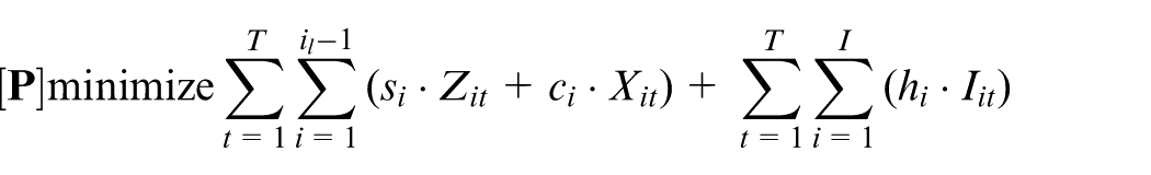
[P] minimize \sum_{t = 1}^{T} \sum_{i = 1}^{i_{l} - 1} (s_{i} \cdot Z_{it} + c_{i} \cdot X_{it}) + \sum_{t = 1}^{T} \sum_{i = 1}^{I} (h_{i} \cdot I_{it})

subject to

I_{i t} = I_{i, t - 1} + R_{i t} - X_{i t} for all i = 1, 2, \dots, i_{r} and t = 1, 2, \dots, T

(1)

I_{i t} = I_{i, t - 1} + \sum_{j \in Φ_{(i)}} a_{j i} \cdot X_{j k} - X_{i t} - d_{i t} for all i = i_{r + 1}, \dots, i_{l - 1} and t = 1, 2, \dots, T

(2)

I_{i t} = I_{i, t - 1} + \sum_{j \in Φ_{(i)}} a_{j i} \cdot X_{j t} - d_{i t} for all i = i_{l}, \dots, I and t = 1, 2, \dots, T

(3)

X_{it} \leq M \cdot Z_{it} for all i = 1, 2, \dots, {i_{l}}_{- 1} and t = 1, 2, \dots, T

(4)

X_{it}, I_{it} \in Z^{+} for all i = 1, 2, \dots, {i_{l}}_{- 1} and t = 1, 2, \dots, T

(5)

Z_{it} \in {0, 1} for all i = 1, 2, \dots, {i_{l}}_{- 1} and t = 1, 2, \dots, T

(6)

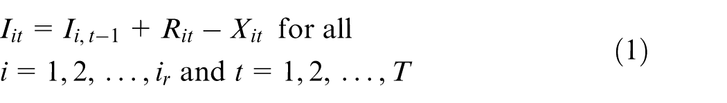
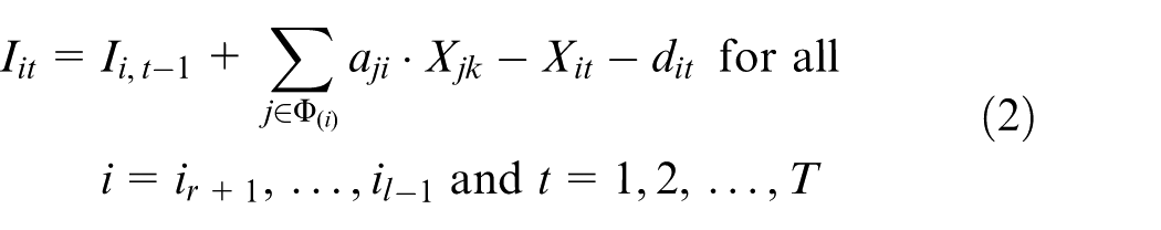
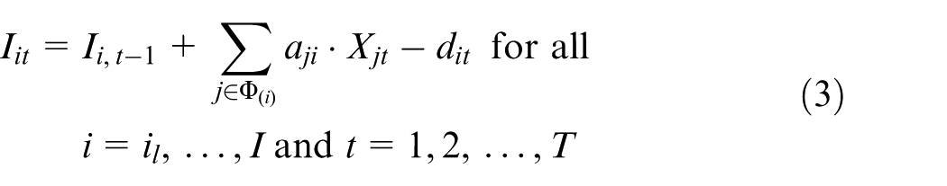
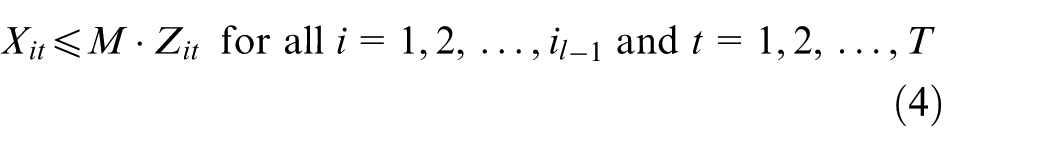
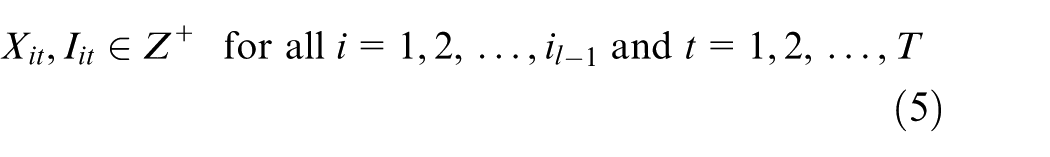
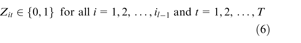
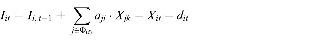
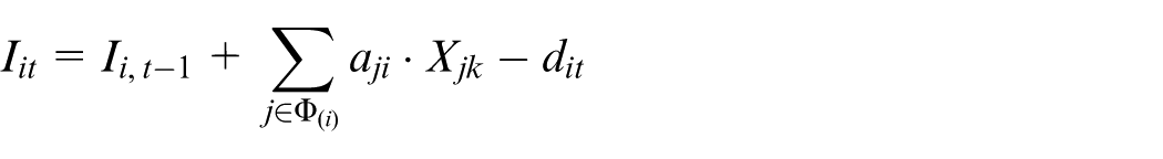
The objective function denotes the total cost, that is, the sum of setup, operation and inventory holding costs over the planning horizon. Constraints (1), (2) and (3) represent the inventory balance of each item. More specifically, constraint (1) denotes the inventory balance for root items. In other words, at the end of each period, the inventory level of each root item is what we had the period before, increased by the amount of the root item collected in that period and decreased by the quantity of the root item disassembled in that period. Similarly, constraints (2) and (3) represent the inventory balances of subassemblies (intermediate items) and parts (leaf items). Constraint (4) ensures that a setup cost be incurred in a period when there is at least one disassembly operation in that period. Finally, constraints (5) and (6) represent the integer conditions of decision variables.

As explained earlier, the model [P] is a multi-period extension of the single-period model of Kang et al.¹³ Since Kang et al.¹³ prove that the single-period model with parts commonality is NP-hard, we can easily see that the model [P] is also NP-hard. Note that the parts commonality increases the problem complexity significantly since it gives alternative procurement sources for each common item and hence creates additional interdependencies among items.¹²

Two-phase heuristic algorithm

As explained earlier, the solution algorithm consists of two phases: (a) obtaining an initial solution and (b) improvement. Before explaining the detailed procedure, an overview of the two-phase heuristic is shown in Figure 3.

Figure 3.

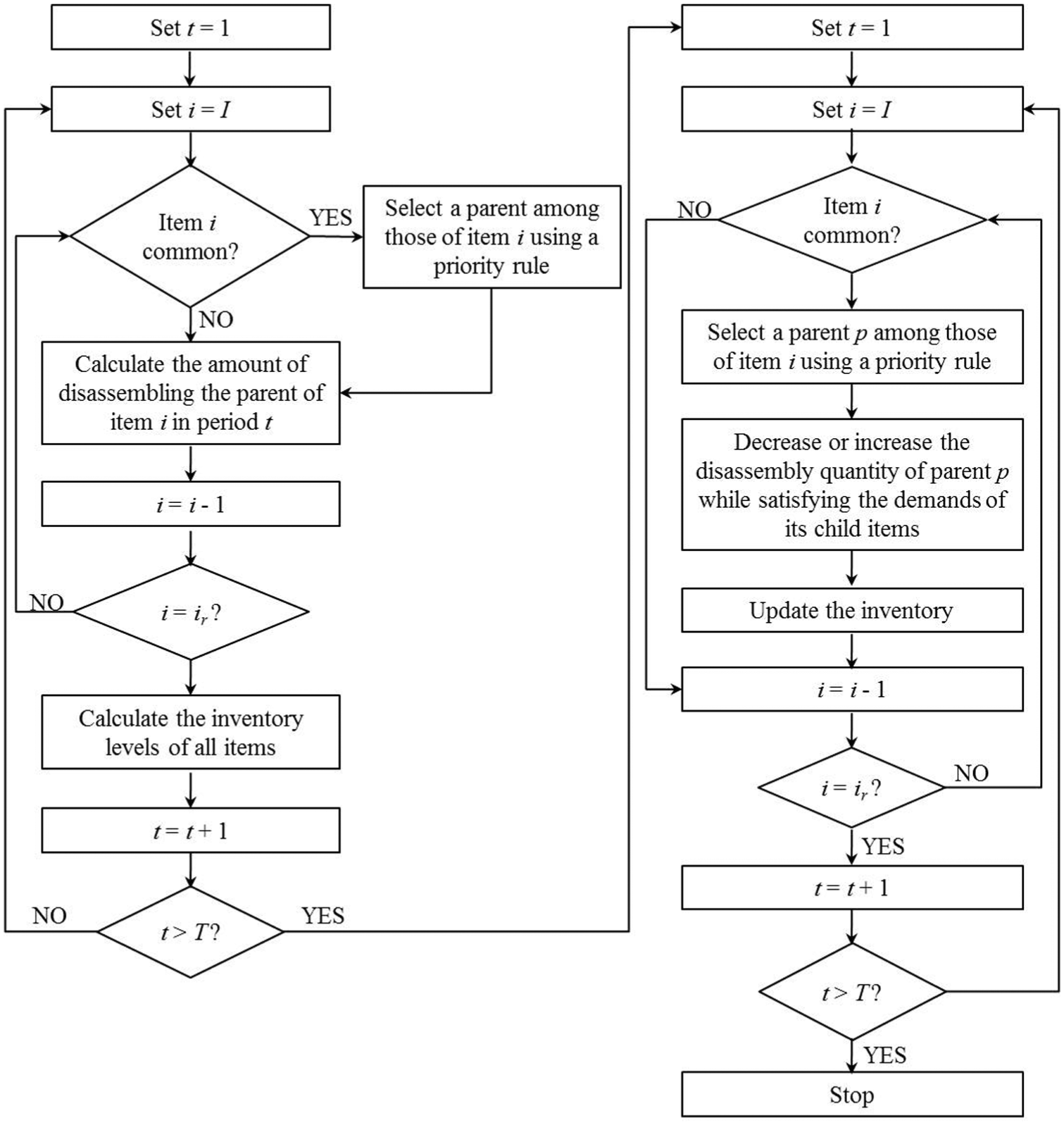
Two-phase heuristic: overview.

Phase 1: obtaining an initial solution

The initial solution is obtained by the priority-based greedy heuristic that determines the amounts of disassembling parent items that satisfy the demands of their child items from the first to the last period. Note that the remaining ones after satisfying the demands of an item in a period can be carried over to the next period.

As can be seen in Figure 3, the demand of each item is satisfied sequentially from the largest to the smallest indexed item. Here, two cases, common and non-common items, are considered.

Case 1 (common items)

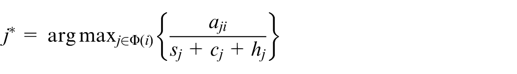
If the current item i is common, a parent item is selected among those associated with the current common item using a priority rule, that is, the maximum ratio of the yield divided by the sum of setup, operation and inventory holding costs. More formally, selected is the parent item j* such that

j^{*} = \arg {max}_{j \in Φ (i)} {\frac{a_{ji}}{s_{j} + c_{j} + h_{j}}}

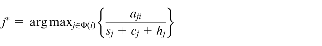
where Φ(i) and a_ji denote the set of parents of item i and the yield of item i obtained from disassembling one unit of parent item j, respectively. After selecting a parent item j*, its disassembly quantity is calculated as the actual demand of the current common item i divided by the yield, that is

X_{j^{*} t} = ⌈ \frac{A D_{it}}{a_{j^{*} i}} ⌉

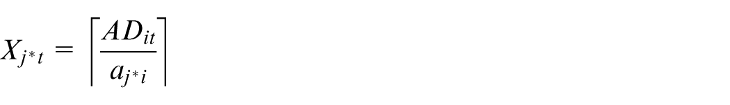
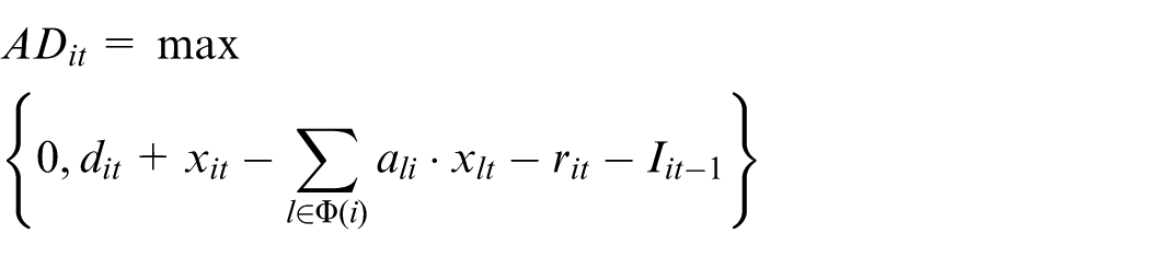
where ⌈•⌉ is the smallest integer that is greater than or equal to •. Also, the actual demand (AD_it) of item i in period t can be calculated as follows

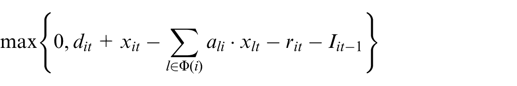
max {0, d_{it} + x_{it} - \sum_{l \in Φ (i)} a_{li} \cdot x_{lt} - r_{it} - I_{it - 1}}

That is, the sum of the demand and the disassembly quantity subtracted by the sum of the amount of the common items obtained from disassembling the other parents, the scheduled receipts of the item (if any) and its inventory carried over from the directly preceding period.

Case 2 (non-common items)

If the current item i is not common, we can specify its unique parent item j* from which the item i can be obtained. Then, its disassembly quantity can be calculated as in the non-common item case.

Now, the detailed procedure to obtain the initial solution is summarized below.

Procedure 1. (Obtaining an initial solution)

Step 1. Set t = 1.

Step 2. Set i = I, that is, the item with the largest index.

Step 3. Identify the parent of item i and its disassembly quantity using the following steps.

If the current item i is common, select a parent item j* such that

j^{*} = \arg max_{j \in Φ (i)} {\frac{a_{ji}}{s_{j} + c_{j} + h_{j}}}

among those associated with the current common item. Otherwise, set the parent item to be its parent item, let it be j*.

Determine the disassembly quantity of the selected parent j* as X_j*t = ⌈AD_it/a_j*i⌉, where

A D_{i t} = \max {0, d_{i t} + x_{i t} - \sum_{l \in Φ (i)} a_{l i} \cdot x_{l t} - r_{i t} - I_{i t - 1}}

Step 4. Set i = i₋1. If i = i_r, that is, the root item with the largest index, go to Step 5. Otherwise, go to Step 3.

Step 5. Calculate the inventory level (I_it) of each item remained after satisfying the demand of that item in period t as follows. The following three cases are considered.

Case 1: If item i is the root, $I_{it} = I_{i, t - 1} + R_{it} - X_{it}$ .

Case 2: Else if item i is a parent (not the root)

I_{it} = I_{i, t - 1} + \sum_{j \in Φ_{(i)}} a_{ji} \cdot X_{jk} - X_{it} - d_{it}

Case 3: Otherwise (item i is a leaf)

I_{it} = I_{i, t - 1} + \sum_{j \in Φ_{(i)}} a_{ji} \cdot X_{jk} - d_{it}

Step 6. Set t = t+1. If t > T, stop. Otherwise, go to Step 2.

Phase 2: improvement

After obtaining an initial solution, it is improved in the second phase. The basic idea is to remove unnecessary disassembly operations while satisfying the component demands.

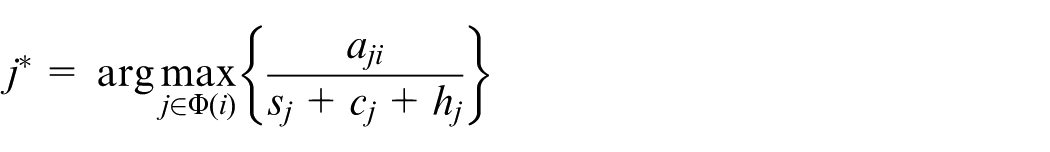
The unnecessary disassembly operations are specified for each module with multiple parent items and one common child item. More specifically, for a common item i, a parent item is selected among those associated with the common item using a priority rule explained earlier, that is, parent item j* is selected such that

j^{*} = \arg {max}_{j \in Φ (i)} {\frac{a_{ji}}{s_{j} + c_{j} + h_{j}}}

Then, the amount of disassembling the parent item j* is decreased or increased to the minimum one that satisfies the demand requirements of its child items.

Now, the details of the improvement procedure are summarized below.

Procedure 2. (Improvement)

Step 1. Set t = 1.

Step 2. Set i = I, that is, the item with the largest index.

Step 3. If item i is not common, go to Step 4. Otherwise, select a parent item j* such that

j^{*} = \arg max_{j \in Φ (i)} {\frac{a_{ji}}{s_{j} + c_{j} + h_{j}}}

Then, if there is a surplus inventory of item i in period t, that is I_it ≥ d_it, set X_j*t = X_j*t₋q, where q denotes the maximum amount of decrease in disassembling parent item j* while satisfying the demands of its child items. Otherwise, set X_j*t = X_j*t+q′, where q′ denotes the minimum amount of increase in disassembling parent item j* while satisfying the demands of its child items. Then, update the inventory levels of the child items at the end of period t.

Step 4. Set i = i − 1. If i = i_r, that is, the root item with the largest index, go to Step 5. Otherwise, go to Step 3.

Step 5. Set t = t+1. If t > T, stop. Otherwise, go to Step 2.

Numerical example

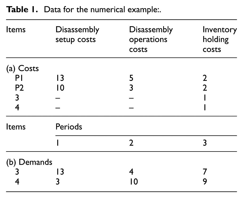
This section illustrates the two-phase heuristic using a simple three-period example for two product types. The d-BOM structure and the relevant data are shown in Figure 4 and Table 1, respectively. As can be seen in the figure, items 1 and 2 are root items, and items 3 and 4 are leaf items. Of the two leaf items, item 4 is a common item since it has two parents, that is, items 1 and 2. Without loss of generality, it is assumed that the amounts of returns for the two product types are large enough to satisfy the demands.

Figure 4.

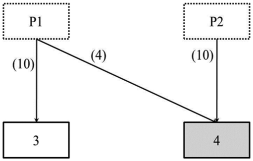
d-BOM structure of the numerical example.

Table 1.

Data for the numerical example:.

Items	Disassembly setup costs	Disassembly operations costs	Inventory holding costs
(a) Costs
P1	13	5	2
P2	10	3	2
3	–	–	1
4	–	–	1
Items	Periods
	1	2	3
(b) Demands
3	13	4	7
4	3	10	9

First, the initial solution can be obtained as follows.

Step 1. Set t = 1.

Step 2. Set i = 4.

Step 3.

Since item 4 is common, item P2 is selected as its parent since

\arg \max {\frac{4}{13 + 5 + 2}, \frac{10}{10 + 3 + 2}} = {\frac{1}{5}, \frac{2}{3}} = 2

Disassembly quantity of the selected parent item P2 becomes 1, that is, X₂₁ = ⌈3/10⌉ = 1. (Note that the actual demand of item 4 is 3.)

Step 4. Set i = 4 − 1 = 3.

Step 3.

Since item 3 is not common, item P1 is selected as its parent.

Disassembly quantity of the parent item P1 becomes 2, that is, X₁₁ = ⌈13/10⌉ = 2.

Step 4. Set i = 3 − 1 = 2. Since i = 2 (index for the last root item), go to Step 5.

Step 5. Calculate the inventory levels of the root and the other items as follows

I₁₁ = I₁₀+R₁₁+X₁₁ = 0+5 − 2 = 3

I₂₁ = I₂₀+R₂₁+X₂₁ = 0+5 − 1 = 4

I₃₁ = I₃₀+a₁₃ · X₁₁ − d₃₁ = 0+20 − 13 = 7

I₄₁ = I₄₀+(a₁₄ · X₁₁+a₂₄ · X₁₂) − d₄₁ = 0+(8+10) − 3 = 15

Step 6. Set t = 1+1 = 2. Since t = 2 ≤ 3, go to Step 2.

Step 2. Set i = 4.

Step 3.

Since item 4 is common, item P2 is selected as its parent since

\arg \max {\frac{4}{13 + 5 + 2}, \frac{10}{10 + 3 + 2}} = {\frac{1}{5}, \frac{2}{3}} = 2

Disassembly quantity of the selected parent item P2 becomes 0, that is, X₂₂ = ⌈0/10⌉ = 0. (Note that the actual demand of item 4 is 0.)

Step 4. Set i = 4 − 1 = 3.

Step 3.

Since item 3 is not common, item P1 is selected as its parent.

Disassembly quantity of the parent item P1 becomes 0, that is, X₁₂ = ⌈0/10⌉ = 0.

Step 4. Set i = 3 − 1 = 2. Since i = 2 (index for the last root item), go to Step 5.

Step 5. Calculate the inventory levels of the root and the other items as follows

I₁₂ = I₁₁+R₁₂ − X₁₂ = 3+5 − 0 = 8

I₂₂ = I₂₂+R₂₂ − X₂₂ = 4+5 − 0 = 9

I₃₂ = I₃₁+a₁₃ · X₁₂ − d₃₂ = 7+0 − 4 = 3

I₄₂ = I₄₁+(a₁₄ · X₁₂ + a₂₄ · X₂₂) − d₄₂ = 15+(0+0) − 10 = 5

Step 6. Set t = 2+1 = 3. Since t = 3 ≤ 3, go to Step 2.

Step 2. Set i = 4.

Step 3.

Since item 4 is common, item P2 is selected as its parent since

\arg \max {\frac{4}{13 + 5 + 2}, \frac{10}{10 + 3 + 2}} = {\frac{1}{5}, \frac{2}{3}} = 2

Disassembly quantity of the selected parent item P2 becomes 1, that is, X₂₃ = ⌈4/10⌉ = 1. (Note that the actual demand of item 4 is 4.)

Step 4. Set i = 4 − 1 = 3.

Step 3.

Since item 3 is not common, item P1 is selected as its parent.

Disassembly quantity of the parent item P1 becomes 1, that is, X₁₃ = ⌈4/10⌉ = 1.

Step 4. Set i = 3 − 1 = 2. Since i = 2 (index for the last root item), go to Step 5.

Step 5. Calculate the inventory levels of the root and the other items as follows

I₁₃ = I₁₂+R₁₃ − X₁₃ = 8+5 − 1 = 12

I₂₃ = I₂₂+R₂₃ − X₂₃ = 9+5 − 1 = 13

I₃₃ = I₃₂+a₁₃ · X₁₃ − d₃₃ = 3+10 − 7 = 6

I₄₃ = I₄₂+(a₁₄ · X₁₃+a₂₄ · X₂₃) − d₄₃ = 5+(4+10) − 9 = 10

Step 6. Set t = 3+1 =4. Since t = 4 > 3, stop.

Then, the initial solution is improved as follows.

Step 1.Set t = 1.

Step 2.Set i = 4, that is, the item with the largest index

Step3.Since item 4 is common, parent item P2 is selected since

\arg \max {\frac{4}{13 + 5 + 2}, \frac{10}{10 + 3 + 2}} = {\frac{1}{5}, \frac{2}{3}} = 2

Then, the amount of decrease in disassembling parent item P2 without violating the demand requirement of item 4 becomes 1, that is, q = 1, and hence, set X₂₁ = 1 − 1 = 0. Then, update the inventory levels of the child items at the end of period t as follows

I₁₁ = 3, I₂₁ = 5, I₃₁ = 7 and I₄₁ = 5

Step4.Set i = 4 − 1 = 3.

Step3.Since item 3 is not common, go to Step 4.

Step4.Set i = 3 − 1 = 2. Since i = 2 (root item with the largest index), go to Step 5.

Step5.Set t = 1+1 = 2. Since t = 2 ≤ 3, go to Step 2.

Step2.Set i = 4.

Step3.Since item 4 is common, parent item P2 is selected since

\arg max {\frac{4}{13 + 5 + 2}, \frac{10}{10 + 3 + 2}} = {\frac{1}{5}, \frac{2}{3}} = 2

Then, the amount of increase in disassembling parent item P2 without violating the demand requirement of item 4 becomes 1, that is, q′ = 1, and hence, set X₂₂ = 0+1 = 1. Then, update the inventory levels of the child items at the end of period t as follows

I₁₂ = 8, I₂₂ = 8, I₃₂ = 3 and I₄₂ = 5

Step4.Set i = 4 − 1 = 3.

Step3.Since item 3 is not common, go to Step 4.

Step4.Set i = 3 − 1 = 2. Since i = 2 (root item with the largest index), go to Step 5.

Step5.Set t = 2+1 = 3. Since t = 3 ≤ 3, go to Step 2.

Step2.Set i = 4.

Step3.Since item 4 is common, parent item P2 is selected since

\arg max {\frac{4}{13 + 5 + 2}, \frac{10}{10 + 3 + 2}} = {\frac{1}{5}, \frac{2}{3}} = 2

Then, the amount of decrease in disassembling parent item P2 without violating the demand requirement of item 4 becomes 1, that is, q = 1, and hence, set X₂₃ = 1 − 1 = 0. Then, update the inventory levels of the child items at the end of period t as follows

I₁₃ = 12, I₂₃ = 14, I₃₃ = 6 and I₄₃ = 0

Step 4. Set i = 4 − 1 = 3.

Step 3. Since item 3 is not common, go to Step 4.

Step 4. Set i = 3 − 1 = 2. Since i = 2 (root item with the largest index), go to Step 5.

Step 5. Set t = 3+1 = 4. Since t = 4 > 3, stop. The final solution becomes ÿ£(X₁₁, X₂₁), (X₁₂, X₂₂), (X₁₃, X₂₃) = ÿ£(2, 0), (0, 1), (1, 0)ÿ§.

Computational results

To test the performance of the two-phase heuristic, computational experiments were performed on randomly generated test instances and the test results are reported in this section. The heuristic was coded in C and the tests were done on a personal computer with an Intel Core2 Quad 3.00 GHz clock speed.

Two performance measures were used in this test: (a) percentage deviations (without and with improvement method) from the optimal solution values or lower bounds and (b) computation time. Here, optimal solutions or lower bounds were obtained from solving the integer programming model [P] directly using CPLEX 11.0, a commercial integer programming software package. More formally, the percentage deviation for an instance is calculated as follows

100 \times (\frac{C_{h} - C_{b}}{C_{b}})

where C_h is the solution value obtained from the heuristic and C_b is the optimal solution value or lower bound. Note that the lower bound was used instead of optimal solution values when CPLEX could not solve the instances in 3600 s.

For the test, we used the 810 randomly generated test instances of Kim and Lee,⁵⁴ our earlier conference paper. The test instances are 10 instances for each of the three levels of the product types (3, 4 and 5), three levels of the number of items (30, 40 and 50), three levels of the planning horizon (3, 5 and 7) and three levels of the percentage of common items (1%, 2% and 5%). For the earlier test, the detailed data were generated as follows. For each level of the number of items, we generated 10 d-BOM structures in which the number of child items for each parent was generated from DU(1, 10). Here, DU(a, b) implies the discrete uniform distribution with [a, b]. Also, the common items were randomly connected to its parents. The demands (d_it) of items in each period were generated from DU(0, 100) and the yields (a_ij) from parent items were generated from DU (1, 10). Finally, setup, operation and inventory holding costs were generated form DU(10, 30), DU(1, 5) and DU (1, 20), respectively.

Test results are summarized in Table 2 that show the average percentage deviations for each level of the number of product types. It can be seen from the table that initial phase gives reasonable quality solutions although it is simple. In fact, the overall average percentage deviations were 2.47%, 2.71% and 3.36% when the percentages of common items are 1%, 2% and 5%, respectively. Also, the overall average percentage deviations after applying the improvement phase were 1.48%, 1.56% and 1.69%, respectively. This shows the effectiveness of the improvement phase. As can be seen in the tables, the performance of the two-phase heuristic gets worse as the percentage of common items increases. Figure 5 shows the overall test results graphically. Finally, the heuristic gave solutions for all the test instances within 0.1 s, and hence it can be applied to practical situations in which the computation time is very critical.

Table 2.

Performance of the two-phase heuristic:.

Number of items	Number of periods	Percentage of common items
		1%		2%		5%
		INI^a	IMP^b	INI	IMP	INI	IMP
(a) Three producttypes
30	3	0.68^c (0.00, 1.76)	0.20 (0.00, 0.78)	0.87 (0.00, 1.87)	0.34 (0.00, 1.71)	2.79 (0.48, 3.63)	0.92 (0.00, 2.82)
	5	1.77 (0.24, 2.93)	0.55 (0.00, 2.23)	2.26 (0.66, 4.35)	0.96 (0.00, 4.35)	2.65 (0.13, 4.91)	1.64 (0.06, 3.30)
	7	2.03 (0.01, 3.93)	1.67 (0.01, 3.49)	3.31 (0.00, 5.32)	1.95 (0.00, 5.00)	3.99 (1.07, 7.70)	2.18 (0.11, 7.49)
40	3	1.97 (0.56, 2.84)	1.07 (0.18, 1.99)	2.75 (0.95, 4.13)	0.66 (0.04, 2.42)	3.04 (0.43, 4.81)	0.76 (0.00, 2.25)
	5	2.77 (0.46, 5.54)	1.31 (0.09, 3.89)	2.45 (0.39, 6.36)	1.66 (0.09, 4.34)	3.14 (0.36, 8.14)	1.62 (0.28, 4.65)
	7	3.57 (1.81, 4.39)	2.90 (0.00, 4.38)	3.39 (0.90, 6.01)	2.48 (0.22, 5.14)	3.41 (0.21, 6.37)	1.87 (0.01, 5.37)
50	3	1.97 (0.02, 5.11)	1.28 (0.02, 4.23)	2.83 (0.67, 4.07)	1.20 (0.19, 2.81)	4.18 (1.61, 6.02)	1.82 (0.13, 4.07)
	5	2.87 (1.35, 5.20)	1.52 (0.00, 4.55)	2.99 (0.48, 4.87)	2.02 (0.00, 4.28)	3.96 (1.43, 7.20)	1.78 (0.18, 4.49)
	7	2.33 (0.35, 5.26)	1.99 (0.17, 5.26)	2.47 (0.86, 4.74)	1.84 (0.09, 4.26)	3.74 (0.44, 7.36)	2.66 (0.01, 5.91)
Average		2.22	1.39	2.59	1.46	3.43	1.69
(b) Four producttypes
30	3	1.35(0.03, 2.48)	0.55(0.00, 1.99)	1.53(0.05, 4.93)	1.53(0.05, 4.93)	1.96(0.03, 3.94)	1.49(0.03, 3.63)
	5	2.18(0.00, 3.76)	1.28(0.00, 3.40)	2.21(0.00, 4.32)	1.10(0.00, 2.55)	2.78(0.60, 4.69)	1.24(0.33, 2.06)
	7	2.76(1.19, 4.86)	1.38(0.02, 2.95)	2.78(0.01, 9.13)	2.22(0.00, 8.69)	2.92(0.43, 4.90)	1.25(0.00, 3.09)
40	3	2.23(0.03, 3.28)	1.35(0.03, 2.78)	2.94(0.18, 5.28)	0.60(0.09, 2.82)	3.86(1.64, 5.32)	1.36(0.19, 3.20)
	5	2.75(0.00, 5.13)	1.55(0.00, 4.13)	2.92(0.17, 5.16)	1.92(0.00, 3.60)	3.94(1.36, 6.78)	2.60(0.21, 6.41)
	7	2.76(0.00, 6.01)	2.00(0.00, 5.04)	2.55(0.34, 9.88)	2.24(0.05, 9.63)	4.03(0.83, 7.75)	2.75(0.79, 6.19)
50	3	2.84(0.02, 5.87)	1.31(0.02, 5.87)	3.19(0.81, 5.44)	1.24(0.07, 3.45)	3.76(1.14, 5.91)	1.48(0.52, 4.27)
	5	3.03(0.77, 6.33)	1.75(0.00, 6.22)	3.27(0.34, 5.75)	1.92(0.04, 5.52)	3.82(1.58, 6.29)	2.14(0.05, 6.13)
	7	3.24(0.40, 6.92)	2.59(0.00, 6.92)	3.56(1.10, 6.77)	2.52(0.08, 5.78)	3.34(0.95, 5.10)	2.26(0.29, 4.35)
Average		2.57	1.53	2.72	1.70	3.37	1.84
(c) Five producttypes
30	3	2.20(0.01, 3.71)	0.97(0.00, 3.33)	2.65(0.00, 5.91)	1.71(0.00, 3.09)	3.09(0.09, 5.68)	0.85(0.00, 1.46)
	5	2.66(0.12, 4.26)	1.70(0.00, 4.11)	2.80(0.00, 4.80)	1.33(0.00, 3.59)	3.08(1.17, 4.32)	1.20(0.00, 3.22)
	7	2.39(0.03, 5.34)	1.29(0.00, 3.22)	2.87(0.60, 4.09)	1.29(0.11, 3.48)	3.22(1.23, 5.23)	1.47(0.02, 3.99)
40	3	2.49(0.14, 4.33)	0.82(0.00, 2.11)	2.91(0.00, 4.43)	1.01(0.00, 3.59)	2.92(0.56, 5.17)	1.64(0.00, 4.27)
	5	2.85(0.28, 4.71)	1.72(0.08, 3.98)	2.87(0.98, 4.93)	1.81(0.62, 4.45)	3.06(1.11, 5.25)	1.42(0.07, 2.85)
	7	2.83(0.28, 5.72)	1.39(0.00, 4.24)	2.76(0.00, 5.36)	1.28(0.00, 3.98)	3.35(0.98, 5.69)	1.90(0.09, 4.61)
50	3	2.56(0.57, 5.50)	1.38(0.13, 4.33)	2.63(0.61, 5.79)	0.75(0.09, 1.74)	3.48(0.67, 5.31)	1.52(0.57, 3.56)
	5	2.53(0.86, 4.70)	2.08(0.14, 3.80)	2.85(0.70, 5.48)	1.93(0.00, 5.39)	3.38(1.82, 4.41)	1.31(0.30, 2.95)
	7	2.99(0.13, 5.96)	2.35(0.00, 5.58)	3.08(0.29, 6.45)	2.50(0.00, 5.42)	3.92(0.32, 9.04)	2.51(0.06, 5.59)
Average		2.61	1.52	2.82	1.51	3.28	1.54

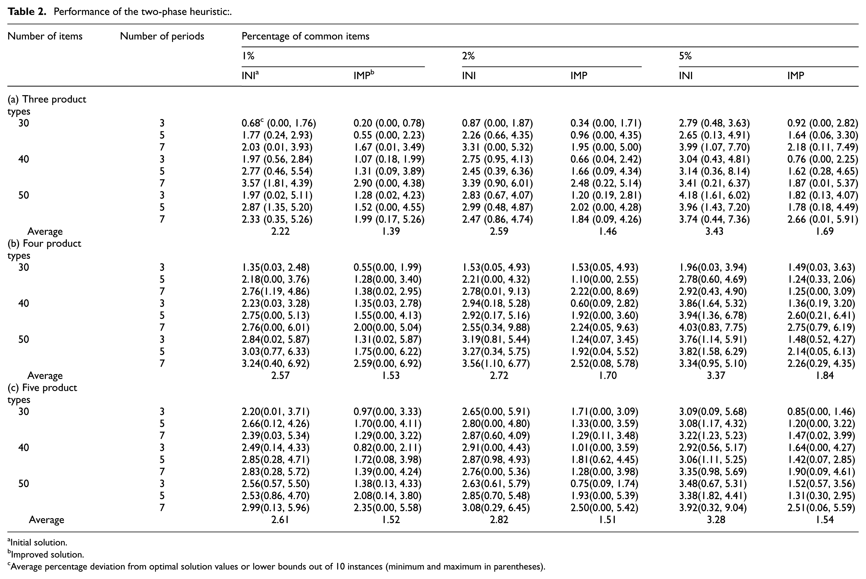
Initial solution.

Improved solution.

Average percentage deviation from optimal solution values or lower bounds out of 10 instances (minimum and maximum in parentheses).

Figure 5.

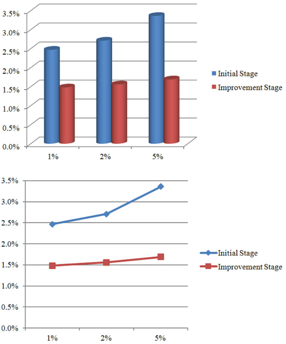
Test results: graphical representation.

Concluding remarks

This study defined a multi-period disassembly levelling and lot-sizing problem for multiple product types with parts commonality. Disassembly levelling is the problem of determining disassembly structures that specify components to be obtained from disassembling end-of-use/life products, and disassembly lot-sizing is the problem of determining the timing and quantity of disassembling products to satisfy the demands of their components. As an extension of the previous study on integrating disassembly levelling and lot-sizing, a multi-period model was suggested to consider the inventory carryovers among different periods of the planning horizon. In particular, we considered the generalized problem in which disassembly levels may be different for products of the same type. To represent the integrated problem, an integer programming model was developed for the objective of minimizing the sum of setup, operation and inventory holding costs. Then, a two-phase heuristic that consists of obtaining an initial solution and improvement was suggested. Finally, computational experiments were done a number of test instances, and the results showed that the two-phase heuristic gives good quality solutions.

As an initial study on multi-period disassembly levelling and lot-sizing, this study can be extended in several directions. First, more sophisticated algorithms, especially improving the initial solution, can be developed after analysing the properties of the problem. Second, other disassembly variables such as disassembly sequence and end-of-life options may be incorporated into the model. For example, in the case of end-of-life options, one can consider the possible ways to deal with surplus inventories. Finally, demand uncertainty is an important further research topic in order to cope with stochastic nature of the second-hand markets.

Footnotes

Acknowledgements

This article is an improved version of the conference paper entitled ‘A heuristic for multi-period disassembly levelling and scheduling’, which was presented at the 2011 IEEE/SICE International Symposium on System Integration, Kyoto, Japan.

Declaration of conflicting interests

The author(s) declared no potential conflicts of interest with respect to the research, authorship and/or publication of this article.

Funding

The author(s) disclosed receipt of the following financial support for the research, authorship, and/or publication of this article: This work was supported by the National Research Foundation of Korea grant funded by Korea government (NRF) (Grant Code: 2011-0015888). This is gratefully acknowledged.

References

Mebratu

. Sustainability and sustainable development: historical and conceptual review. Environ Impact Asses 1998; 18(6): 493–520.

Robèrt

K-H

Schmidt-Bleek

de Larderel

. Strategic sustainable development – selection, design and synergies of applied tools. J Clean Prod 2002; 10(3): 197–214.

Fleischmann

Bloemhof-Ruwaard

Dekker

. Quantitative models for reverse logistics: a review. Eur J Oper Res 1997; 103(1): 1–17.

Bloemhof-Ruwaard

Fleischmann

van Nunen

JAEE

. Reviewing distribution issues in reverse logistics. Lect Notes Econ Math 1999; 480: 23–44.

Srivastava

. Green supply chain management: a state-of-the-art literature review. Int J Manag Rev 2007; 9(1): 53–80.

Lee

D-H

Kim

H-J

Kim

J-S

. Reverse logistics: research issues and literature review. J Korean Inst Ind Eng 2008; 34(3): 270–288.

Sasikumar

Kannan

. Issue in reverse supply chains, part I: end-of-life product recovery and inventory management – an overview. Int J Sustain Eng 2008; 1(3): 154–172.

Sasikumar

Kannan

. Issue in reverse supply chains, part II: reverse distribution issues – an overview. Int J Sustain Eng 2008; 1(4): 234–249.

Jovane

Alting

Armoillotta

. A key issue in product life cycle: disassembly. Ann CIRP 1993; 42(2): 651–658.

10.

Gungor

Gupta

. Issues in environmentally conscious manufacturing and product recovery: a survey. Comput Ind Eng 1999; 36(4): 811–853.

11.

Lee

D-H

Kang

J-G

Xirouchakis

. Disassembly planning and scheduling: review and further research. Proc IMechE, Part B: J Engineering Manufacture 2001; 215(5): 695–710.

12.

Kim

H-J

Lee

D-H

Xirouchakis

. Disassembly scheduling: literature review and further research directions. Int J Prod Res 2007; 45(18–19): 4465–4484.

13.

Kang

K-W

Doh

H-H

Park

J-H

. Disassembly leveling and lot-sizing for multiple product types: a basic model and its extension. Int J Adv Manuf Tech 2016; 82(9–12): 1463–1473.

14.

O’Shea

Grewal

Kaebernick

. State of the art literature survey on disassembly planning. Concurrent Eng: Res A 1998; 6(4): 345–357.

15.

Santoch

Dini

Failli

. Computer aided disassembly planning: state of the art and perspectives. Ann CIRP 2002; 51(2): 507–529.

16.

Lambert

AJD

. Disassembly sequencing: a survey. Int J Prod Res 2003; 41(16): 3721–3759.

17.

Penev

De Ron

. Determination of a disassembly strategy. Int J Prod Res 1996; 34(2): 495–506.

18.

Igarashi

Yamada

Inoue

. 2-stage optimal design and analysis for disassembly system with environmental and economic parts selection using the recyclability evaluation method. Ind Eng Manage Syst 2014; 13(1): 52–66.

19.

Lambert

AJD

. Optimal disassembly of complex products. Int J Prod Res 1997; 35(9): 2509–2523.

20.

Hui

Dong

Guanghong

. A genetic algorithm for product disassembly sequence planning. Neurocomputing 2008; 71(13–15): 2720–2726.

21.

Adenso-Diaz

Garcia-Carbajal

Gupta

. A path-relinking approach for a bi-criteria disassembly sequencing problem. Comput Oper Res 2008; 35(12): 3989–3997.

22.

Jin

Wang

. A systematic selective disassembly approach for waste electrical and electronic equipment with case study on liquid crystal display televisions. Proc IMechE, Part B: J Engineering Manufacture 2017; 231(13): 2261–2278.

23.

Bufardi

Gheorghe

Kiritsis

. A multicriteria decision-aid approach for product end of life alternative selection. Int J Prod Res 2004; 42(16): 3139–3157.

24.

Jun

H-B

Cusin

Kiritsis

. A multi-objective evolutionary algorithm for EOL product recovery optimization: turbocharger case study. Int J Prod Res 2007; 45(18–19): 4573–4594.

25.

Pnueli

Zussman

. Evaluating the end-of-life value of a product and improving it by redesign. Int J Prod Res 1997; 35(4): 921–942.

26.

Johnson

Wang

. Planning product disassembly for material recovery opportunities. Int J Prod Res 1995; 33(11): 3119–3142.

27.

Johnson

Wang

. Economical evaluation of disassembly operations for recycling, remanufacturing and reuse. Int J Prod Res36(12): 3227–3252.

28.

Lambert

AJD

. Linear programming in disassembly/clustering sequence generation. Comput Ind Eng 1999; 36(4): 723–738.

29.

Lambert

AJD

. Exact methods in optimum disassembly sequence search for problems subject to sequence dependent costs. Omega 2006; 34(6): 538–549.

30.

Kang

J-G

Lee

D-H

Xirouchakis

. Parallel disassembly sequencing with sequence-dependent operation times. Ann CIRP 2001; 50(1): 343–346.

31.

Kang

J-G

Lee

D-H

Xirouchakis

. Optimal disassembly sequencing with sequence dependent operation times based on the directed graph of assembly states. J Korean Inst Ind Eng 2002; 28(3): 264–273.

32.

Vinodh

Nachiappan

Praveen Kumar

. Sustainability through disassembly modeling, planning, and leveling: a case study. Clean Technol Envir 2012; 14(1): 55–67.

33.

Vinodh

Praveen Kumar

Nachiappan

. Disassembly modeling, planning, and leveling for a cam-operated rotary switch assembly: a case study. Int J Adv Manuf Tech 2012; 62(5): 789–800.

34.

Erdos

Kritsis

Xirouchakis

. Modeling and evaluating product end-of-life options. Int J Prod Res 2001; 39(6): 1203–1220.

35.

Teunter

. Determining optimal disassembly and recovery strategies. Omega 2006; 34(6): 533–537.

36.

Behdad

Kwak

M-G

Kim

. Simultaneous selective disassembly and end-of-life decision making for multiple products that share disassembly operations. J Mech Design 2010; 132(4): 1–9.

37.

Y-S

Jun

H-B

Kim

H-W

. Disassembly process planning algorithms for end-of-life product recovery and environmentally conscious disposal. Int J Prod Res 2011; 49(23): 7007–7027.

38.

Lee

D-H

Kim

H-J

Choi

. Disassembly scheduling: integer programming models. Proc IMechE, Part B: J Engineering Manufacture 2004; 218(10): 1357–1372.

39.

Gupta

Taleb

. Scheduling disassembly. Int J Prod Res 1994; 32(8): 1857–1866.

40.

Lee

D-H

Xirouchakis

. A two-stage heuristic for disassembly scheduling with assembly product structure. J Oper Res Soc 2004; 55(3): 287–297.

41.

Kim

H-J

Lee

D-H

Xirouchakis

. A branch and bound algorithm for disassembly scheduling with assembly product structure. J Oper Res Soc 2009; 60(3): 419–430.

42.

Lee

D-H

Xirouchakis

Züst

. Disassembly scheduling with capacity constraints. Ann CIRP 2002; 51(1): 387–390.

43.

Jeon

H-B

Kim

J-G

Kim

H-J

. A two-stage heuristic for disassembly scheduling with capacity constraints. Int J Manag Sci 2006; 12(1): 95–112.

44.

Kim

H-J

Lee

D-H

Xirouchakis

. Two-phase heuristic for disassembly scheduling with multiple product types and parts commonality. Int J Prod Res 2006; 44(1): 195–212.

45.

Taleb

Gupta

Brennan

. Disassembly of complex product structures with parts and materials commonality. Prod Plan Control 1997; 8(3): 255–269.

46.

Taleb

Gupta

. Disassembly of multiple products structure. Comput Ind Eng 1997; 32(4): 949–961.

47.

Lambert

AJD

Gupta

. Demand-driven disassembly optimization for electronic products. J Electron Manuf 2002; 11(2): 121–135.

48.

Kim

H-J

Lee

D-H

Xirouchakis

. Disassembly scheduling with multiple product types. Ann CIRP 2003; 52(1): 403–406.

49.

Kim

J-G

Jeon

H-B

Kim

H-J

. Disassembly scheduling with capacity constraints: minimizing the number of products disassembled. Proc IMechE, Part B: J Engineering Manufacture 2006; 220(9): 1473–1481.

50.

Langella

. Heuristics for demand-driven disassembly planning. Comput Ind Eng 2007; 34(2): 552–577.

51.

Veerakamolmal

Gupta

. Optimal analysis of lot size balancing for multi-products selective disassembly. Int J Flex Autom Integr Manuf 1998; 6: 245–269.

52.

Kongar

Gupta

. A disassembly to order system under uncertainty. Omega 2006; 34(6): 550–561.

53.

Xanthopoulos

Iakovou

. On the optimal design of the disassembly and recovery processes. Waste Manage 2009; 29(5): 1702–1711.

54.

Kim

D-H

Lee

D-H

. A heuristic for multi-period disassembly levelling and scheduling. In: Proceedings of the IEEE/SICE international symposium on system integration, Kyoto, Japan, 20–22 December 2011. New York: IEEE.

Multi-period disassembly levelling and lot-sizing for multiple product types with parts commonality

Abstract

Keywords

Introduction

Literature review

Disassembly process planning

Disassembly lot-sizing

Disassembly process planning and lot-sizing

Problem description

Two-phase heuristic algorithm

Phase 1: obtaining an initial solution

Case 1 (common items)

Case 2 (non-common items)

Phase 2: improvement

Numerical example

Computational results

Concluding remarks

Footnotes

Acknowledgements

Declaration of conflicting interests

Funding

References