Empirical modeling of compressive residual stress profile in shot peening TC17 alloy using characteristic parameters and sinusoidal decay function

Abstract

This article introduces two comprehensive experimental models to predict the compressive residual stress profile induced in TC17 alloy after shot peening. Experiments are carried out utilizing one of experimental design techniques based on response surface methodology. Shot peening intensity and coverage are considered as two input parameters affecting compressive residual stress profile. The characteristic parameters model is created by regression analysis, which has the capability of predicting the four main characteristic parameters of a typical compressive residual stress profile. Based on this model, the absolute sensitivity of characteristic parameters with respect to shot peening intensity and coverage is analyzed. The sinusoidal decay function model is created with a proposition of that the compressive residual stress profile is a sinusoidal decay function of the depth beneath surface and the coefficients of this function are, in turn, functions of the two input shot peening parameters. The main advantage of sinusoidal decay function model over characteristic parameters model is that it provides the effect of shot peening parameters on the shape of the compressive residual stress profile. The two models have been checked for accuracy by two extra tests. The results show that the prediction errors of the four main characteristic parameters are within 20%, and the compressive residual stress profiles predicted by the sinusoidal decay function model are in consistent with experimental data.

Introduction

TC17 titanium alloy is a kind of “beta-rich” alpha–beta two-phase high-strength titanium alloy with many advantageous properties, such as high specific strength, good plastic and fracture toughness, high hardenability, and wide forging temperature. ¹ This alloy can meet the demands of damage tolerance design, high frame benefit, high reliability, and low manufacturing cost. Consequently, it has become essential for the aircraft engine components manufacturing such as fan disk, compressor disk, and centrifugal impeller. However, the fatigue property of this alloy is very sensitive to surface condition due to its high strength, which may decrease the fatigue life significantly and affect the safe reliability of the aircraft engine. Therefore, various surface modification by mechanical treatment such as shot peening (SP), laser shock peening, deep rolling, roller burnishing, and ultrasonic impact treatment and have been studied and applied for the improvement of fatigue property of high-strength alloy.^2–7 Among these techniques, SP is most commonly used due to its low cost and can be used on small or large areas depending on requirements.

In the processing of SP, enormous quantity of small spherical particles, typically made of hard steel, ceramic, or glass, are made to impact the surface of the structural component at high velocities. As a result, intense local plastic deformation is imposed within a thin layer beneath the surface. Meanwhile, high compressive residual stress and refined grains are introduced within the surface deformation layer, which can enhance the fatigue life and stress corrosion resistance of components. ⁸ The compressive residual stress is usually regarded as the major factor in increasing fatigue life, which can move the crack initiation from surface to subsurface and resist to crack propagation due to the higher level of crack closure effect, thus the fatigue life can be increased significantly. ⁹ Generally, compressive residual stress is directly determined by the parameters of SP; therefore, it is significant to investigate the relationship between compressive residual stress profile (CRSP) and SP parameters.

A literature survey shows that work on the CRSP introduced by SP has been conducted by many researchers. As early as 1944, the “Almen intensity” invented by Almen ¹⁰ was used to predict the result of residual stress after SP. Although the standardized Almen intensity measurement is well documented, and widely used, it may not reveal the difference between SP parameters, such as the same intensity can be obtained by small shot thrown at high velocity or by large shot thrown at lower velocity. ¹¹ Finite element modeling is a way of investigating the effect of SP parameters on surface residual stress as well as CRSP. Different types of finite element models of shots and targets have been created to simulate the SP process. A three-dimensional (3D) model with two symmetry surfaces, ¹² a 3D model with an equilateral triangle impact surface and three symmetry surfaces, ¹³ a 3D model with strain rate sensitive material properties as well as work hardening material properties, ¹⁴ a half circular 3D finite element model with one symmetry surface, ¹⁵ a 3D model without symmetry boundary condition, ¹⁶ and a 3D cell model with a square contact surface and four symmetry surfaces ¹⁷ were developed subsequently to predict SP-induced CRSP. In order to understand the progress from a single impact to multiple impacts, an artificially designed series of impacts was modeled. ¹⁸ These efforts usually provide a good understanding of the SP process and represent the CRSP clearly. However, many assumptions are involved in these models, and even when experimentally validated, they may lack the capability of predicting other tests. In addition, when their predictable precisions are improved by decreasing the element size or time step, the computation cost can be too high to account for their value.

Analytically, modeling is another way to calculate the residual stress using physical equations, where plain strain or plain stress conditions are assumed. According to Hertz elastic contact theory, Iliushin’s elastic–plastic theory and the physical concepts of reversed yielding and hardening, Li et al. ¹⁹ proposed a simplified analytical model for calculating the CRSP induced by SP. Shen and Atluri ²⁰ claimed that the major drawbacks of Li’s analysis were assuming the SP procedure as a static phenomenon and using an empirical relation between the plastic radius of the dent and the equivalent static load of SP. And so to modify Li’s physical model, Shen calculated the plastic indentation using an average pressure distribution and taken the primary SP factors into consideration. Franchim et al. ²¹ made two modifications to the analytical model proposed by Li and complemented by Shen and Atluri, the Hertzian pressure was considered as a dynamic load and the Ramberg–Osgood and/or Ludwick constitutive models of the stress–strain curve was adopted to describe the plastic behavior of target material. Based on the method proposed by Shen and Atluri, Bhuvaraghan et al. ²² used a simplified analytical approach with a simple modification of including the strain rate effects to predict the CRSP. However, the SP process is considerably complex: the system is dynamic and includes contact. These analytical models represent the ideal conditions of events and usually are not practically applicable.

The majority of research existing in literature on the effect of SP parameters on CRSP is experimental in nature. Sridhar et al. ²³ investigated the residual stress distribution of two commercial titanium alloys in the machined and polished as well as the machined, polished, and shot-peened conditions using the method of drilling holes. The influences of mechanical properties of target materials and peening parameters on CRSP were investigated by Gao et al., ²⁴ it was found that the maximum of compressive residual stress is almost the same even under different SP conditions. While Feng et al. ²⁵ found that the value of maximum compressive residual stress reduced significantly when SP intensity was too large. Bendeich et al. ²⁶ carried out the measurements of residual stress using both the neutron diffraction and X-ray diffraction method; the results indicated that the blade surface treated by grit blasting generated a compressive residual stress with a depth of 100 µm. John et al. ²⁷ studied the stability of shot-peen residual stresses in an α + β titanium alloy, approximately 80% of the residual stresses were retained at 399 °C up to 100 h. Tsuji et al. ²⁸ studied the impact of SP using shot particles with a diameter of 70 µm onto the properties of the Ti-6Al-4V titanium alloy surface layer. The results showed that the maximum compressive residual stress of approximately −970 MPa existed at the surface, and the depth of compressive residual stress layer was approximately 100 µm beneath the surface. Xie et al. ²⁹ investigated the CRSP of titanium matrix composites (TiB + TiC)/Ti-6Al-4V after SP, the depths of surface deformation layers of two samples with reinforcements were about 250 µm, and that of the matrix was about 300 µm. Additionally, in the deep surface layer (75–300 µm), the reinforcements made the compressive residual stress to decrease faster than that of matrix. Li et al. ³⁰ investigated the residual stress and microstructure at the different depth of Ti-6Al-4V alloy treated by wet peening process, and the relationship between the CRSP and the microstructural evolution mechanism was elaborated. Yao et al. ³¹ investigated the influence of SP parameters on surface integrity of 7055 aluminum alloy. The results showed that the smaller the surface roughness, the larger the curvature radius of valley bottom, better micro-hardness distribution, and higher surface residual compressive stress would be very important for improving fatigue life.

Most researchers focus on the description and analysis of CRSP, and few investigations have been made on modeling the relationship between CRSP and SP parameters, especially based on experimental data. However, some researchers have modeled the residual stress profile in turning and milling, using statically fitted polynomial function and sinusoidal decay function.^32–34 This work aims to model the CRSP empirically using four main characteristic parameters and a sinusoidal decay function. With the help of these two experimental models, it will become possible to predict the CRSP induced by SP, such that the surface integrity of the shot-peened components for TC17 alloy is maximized under service conditions.

Experiments

Materials

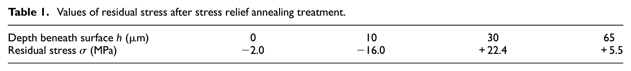
The material used in this investigation was TC17 alloy with a chemical composition of 4.5%–5.5% Al, 1.6%–2.4% Sn, 1.6%–2.4% Zr, 3.5%–4.5% Mo, 3.5%–4.5% Cr, and Ti balance (in wt %). ³⁵ At room temperature, the yield strength of this material was measured at 1030 MPa, and the tensile strength was 1120 MPa. The as-received specimens with section dimensions of 20 mm × 20 mm × 15 mm were mechanically ground to the range of surface roughness 0.165–0.189 µm (Ra). In order to eliminate the initial residual stress, all specimens were annealed at 360 °C for 30 min and followed by annealing at 550 °C for 3–4 h, air cooling. After stress relief annealing, two specimens were selected to measure the residual stresses using X-ray diffraction method. The average value of residual stress is given in Table 1. It reveals that the initial residual stress can be negligible.

Table 1.

Values of residual stress after stress relief annealing treatment.

Depth beneath surface h (µm)	0	10	30	65
Residual stress σ (MPa)	−2.0	−16.0	+22.4	+5.5

SP treatment

All SP tests were carried out on a pneumatic machine using ceramic shots with a hardness of 643–785 HV and a diameter of 0.3 mm. The SP intensity is measured by the arc height of Almen specimen (A type), which is controlled by jet pressure of nozzle, SP time, and diameter of small shots. The diameter of peening nozzle was 8 mm, and the distance between nozzle and specimen was 130 mm. The incident angle was kept at 45°. In this investigation, a response surface methodology with a central composed second-order rotatable design was used. SP intensity and coverage are considered as the independent variables, and their actual and coded values are summarized in Table 2. The coded value of each parameter can be obtained from equation (1)

$$\{\begin{array}{l}{X}_1=\left(f_A-f_{A0}\right)/\left(f_{A+1}-f_{A0}\right)\hfill \\ X_2=\left(C-C_0\right)/\left(C_{+1}-C_0\right)\hfill \end{array}$$

(1)

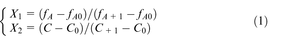
where X₁ and X₂ are the coded values of f_A and C; f_A0 and C₀ are the actual values at center point; and f_A + 1 and C₊₁ are the actual values at high point.

Table 2.

Actual and coded values of SP parameters.

Parameters	Symbol	Levels in code form tab
		−1.41 (Lowest)	−1 (Low)	0 (Center)	+1 (High)	+1.41 (Highest)
SP intensity (mmA)	fA	0.05	0.08	0.15	0.22	0.25
SP coverage (×100%)	C	1.00	1.44	2.50	3.56	4.00

Residual stress measurement

Residual stress was determined using X-ray diffraction with a sin²ψ-method. X-ray diffraction techniques exploit the fact that when a metal is under stress, applied or residual stress, the resulting elastic strains cause the atomic planes in the metallic crystal structure to change their spacing. The elastic strains can be calculated using the theory of elastic mechanics under the presumption of plane stress state, meanwhile the inter-planar spacing d can be directly measured by X-ray diffraction; from this quantity, the total stress on the metal can then be obtained.

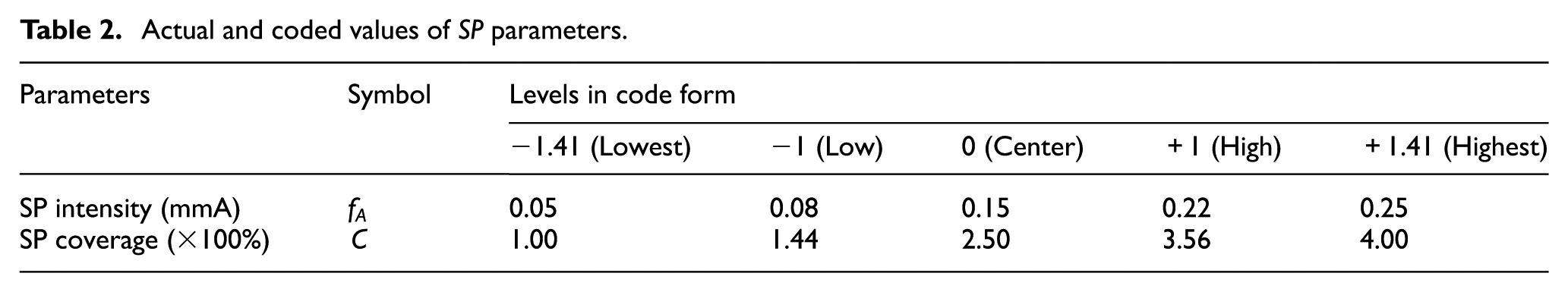
In this article, an X-ray stress analyzer (LXRD, Proto, Canada) was used to measure the residual stress. The system mainly consists of goniometer controller, goniometer head and computer. Two systematic detectors record diffraction information from two opposite directions, and each detector independently employs Gaussian fitting to determine the peak location. The amount of the peak used for fitting is 85%, applied from top to bottom, as shown in Figure 1. In order to improve the accuracy of peak location and stress measurement, background subtraction will be displayed to eliminate the irrelevant factors of Bragg diffraction, as shown in Figure 2. Once the diffraction peak location, that is, the diffraction angle was determined, the inter-planar spacing d could be calculated by Bragg’s equation. After the profiles under nine different ψ angles were collected, the slope M of linear dependence of d-spacing versus sin²ψ was determined with an elliptical fitting method, as shown in Figure 3. Residual stress σ is equal to KM, stress constant K is −252.8 MPa/°. The stress is compressive if the slope M is negative, while it is tensile if the slope M is positive.

Figure 1.

Normalized background fit profile shown with Gaussian peak fitting.

Figure 2.

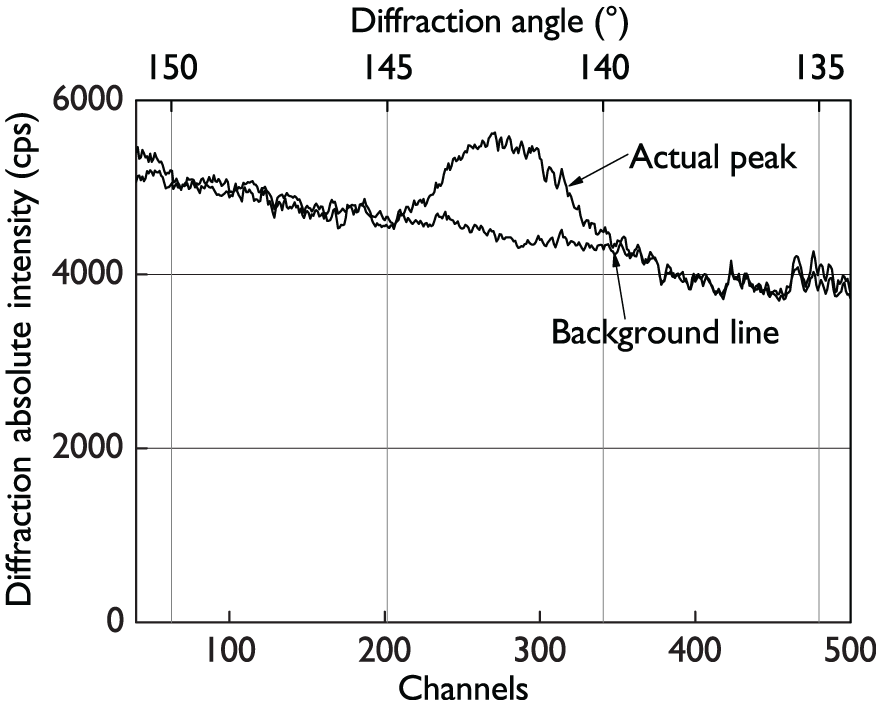
Actual peak collected and background subtraction.

Figure 3.

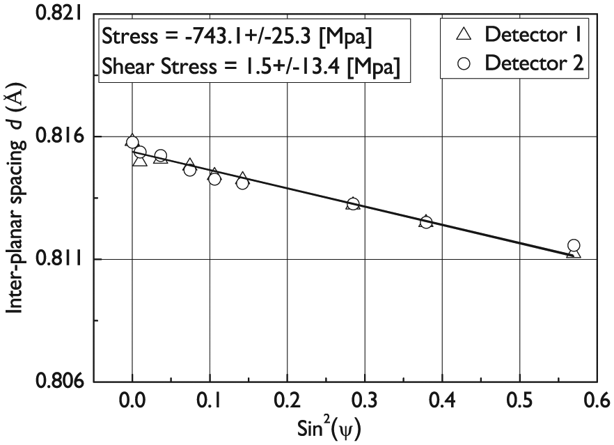
Relation of inter-planar spacing d versus sin²ψ.

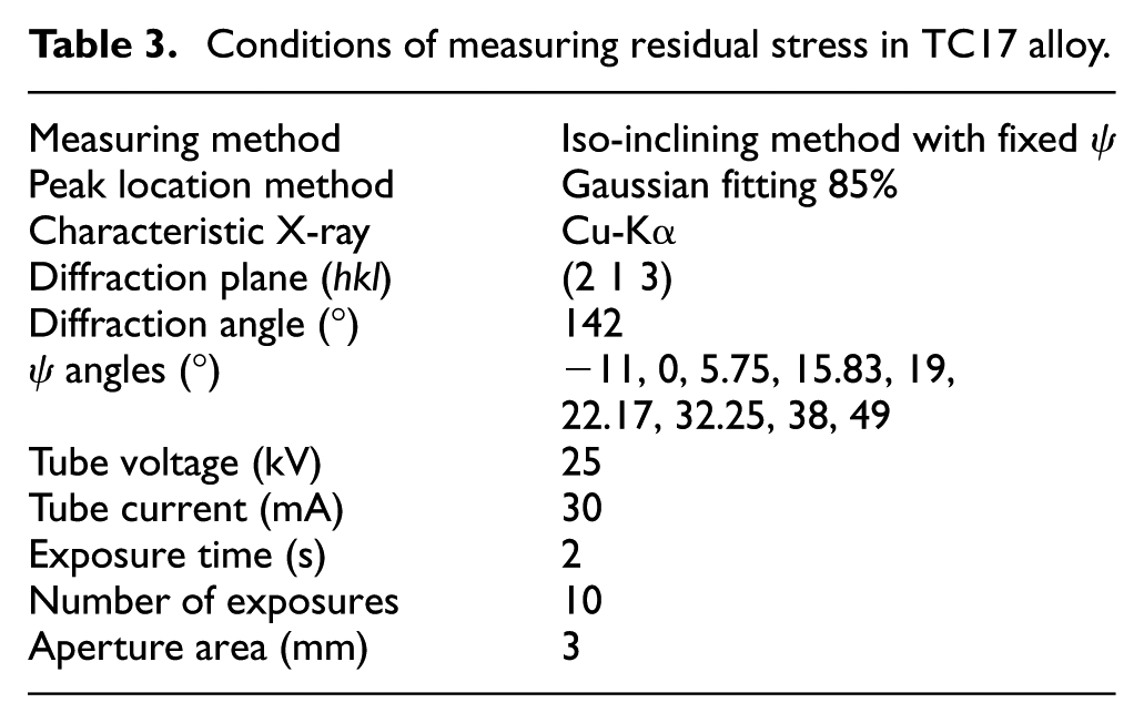
In order to obtain the residual stress distribution in deeper region, the thin top layers were removed one by one via successive electrolytic polishing with a solution of methanol, ethyleneglycol monobutyl ether, and perchloric acid in proportion of 59:35:6. The detailed conditions of measuring residual stress are given in Table 3.

Table 3.

Conditions of measuring residual stress in TC17 alloy.

Measuring method	Iso-inclining method with fixed ψ
Peak location method	Gaussian fitting 85%
Characteristic X-ray	Cu-Kα
Diffraction plane (hkl)	(2 1 3)
Diffraction angle (°)	142
ψ angles (°)	−11, 0, 5.75, 15.83, 19, 22.17, 32.25, 38, 49
Tube voltage (kV)	25
Tube current (mA)	30
Exposure time (s)	2
Number of exposures	10
Aperture area (mm)	φ3

Modeling

Characteristic parameters model

In this article, four main characteristic parameters have been named and investigated: σ_srs, compressive residual stress at surface (MPa); σ_mcrs, maximum compressive residual stress (MPa); Z_m, depth of the maximum residual stress (µm); and Z₀, depth at which residual stress becomes near-zero (µm). These parameters reveal three key points in the CRSP. The experimental design matrix and measured data of characteristic parameters are listed in Table 4.

Table 4.

Experimental design matrix and measured data of characteristic parameters.

Comb. no.	Coded value		Response value
	X 1	X 2	σsrs (MPa)	σmcrs (MPa)	Zm (µm)	Z0 (µm)
1	−1	−1	−673.23	−778.38	10	58
2	1	−1	−701.65	−877.38	20	87
3	−1	1	−679.3	−830.38	12	67
4	1	1	−725.04	−931.71	25	125
5	−1.41	0	−660.97	−766.17	10	47
6	1.41	0	−712.88	−891.31	20	90
7	0	−1.41	−680.12	−859.16	15	70
8	0	1.41	−708.31	−899.83	20	99
9	0	0	−689.23	−878.69	28	87
10	0	0	−698.31	−884.23	23	85
11	0	0	−696.29	−896.35	25	82
12	0	0	−694.71	−917.25	28	84
13	0	0	−688.13	−901.2	30	86

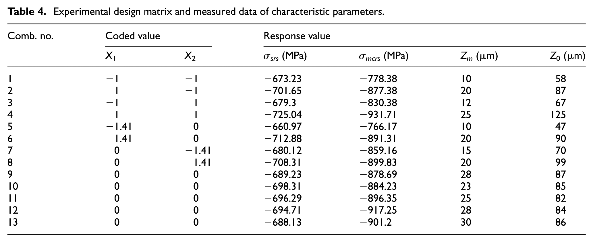
The effect of SP parameters on characteristic parameters is investigated based on second-order response models using least square regression analysis of the data in Table 4. Quadratic models of characteristic parameters are given in equation (2)

$$\{\begin{array}{l}{\sigma }_{srs}=-692.94-18.45X_1-8.67X_2\\ {\sigma }_{mcrs}=-890.02-47.16X_1-20.48X_2+32.28X_1^2\\ Z_m=26.80+4.64X_1+1.76X_2-5.78X_1^2-4.52X_2^2\\ Z_0=86.04+18.48X_1+11.00X_2+7.25X_1{X}_2-6.45X_1^2\end{array}$$

(2)

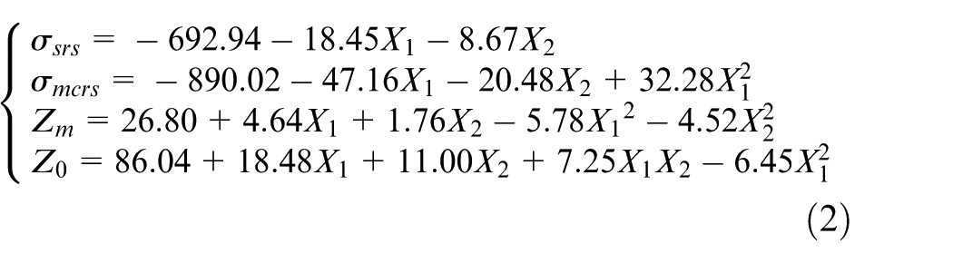
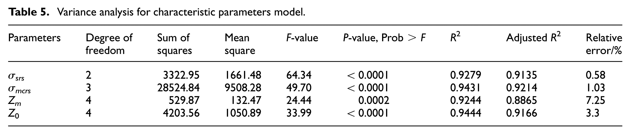
Adequacy of the models has been tested for a 95% confidence interval using Fisher’s test. To decide about the adequacy of the model, sequential model sum of squares, mean squares, and model summary statistics are performed and tabulated subsequently. Table 5 shows the detailed analysis of variance (ANOVA) for characteristic parameters. The ANOVA clearly indicates the “Prob > F” values of σ_srs, σ_mcrs, and Z₀ are < 0.0001, meaning that the models are highly significant; the “Prob > F” value of Z_m is < 0.05, meaning that the model is significant. The coefficient of determination R² is in reasonable agreement with the adjusted R² and the relative error was less than 8%, showing a good fit between prediction values of model and experimental values.

Table 5.

Variance analysis for characteristic parameters model.

Parameters	Degree of freedom	Sum of squares	Mean square	F-value	P-value, Prob > F	R 2	Adjusted R2	Relative error/%
σsrs	2	3322.95	1661.48	64.34	<0.0001	0.9279	0.9135	0.58
σmcrs	3	28524.84	9508.28	49.70	<0.0001	0.9431	0.9214	1.03
Zm	4	529.87	132.47	24.44	0.0002	0.9244	0.8865	7.25
Z 0	4	4203.56	1050.89	33.99	<0.0001	0.9444	0.9166	3.3

Using the sensitivity analysis method, the absolute sensitivity of characteristic parameters model to SP intensity and coverage are shown in equations (3) and (4), respectively. From equation (3), the sensitivity of σ_srs to SP intensity is kept constant; however, the sensitivity of σ_mcrs, Z_m, and Z₀ decreases slightly with the increase in SP intensity. From equation (4), it can be observed that the sensitivity of σ_srs and σ_mcrs remains unchanged, while a slightly decrease is found for the sensitivity of Z_m and Z₀ following the increase in SP coverage. For the parameter range studied, the absolute sensitivity value of σ_mcrs was larger than that of σ_srs in most cases. Compared with Z_m, the absolute sensitivity value of Z₀ was larger too. Thus, compared with σ_srs and Z _m , σ_mcrs and Z₀ are more sensitive to the variations of SP intensity and coverage. The four characteristic parameters are all more sensitive to the variation of SP intensity than that of SP coverage. Thus, a favorable CRSP can be induced by mainly adjusting SP intensity

$$\{\begin{array}{l}\frac{\partial {\sigma }_{srs}}{\partial X_1}=-18.45\\ \frac{\partial {\sigma }_{mcrs}}{\partial X_1}=-47.16+64.56X_1\\ \frac{\partial Z_m}{\partial X_1}=4.64-11.56X_1\\ \frac{\partial Z_0}{\partial X_1}=18.48+7.25X_2-12.90X_1\end{array}$$

(3)

$$\{\begin{array}{l}\frac{\partial {\sigma }_{srs}}{\partial X_2}=-8.67\\ \frac{\partial {\sigma }_{mcrs}}{\partial X_2}=-20.48\\ \frac{\partial Z_m}{\partial X_2}=1.76-9.04X_2\\ \frac{\partial Z_0}{\partial X_2}=11.00+7.25X_1\end{array}$$

(4)

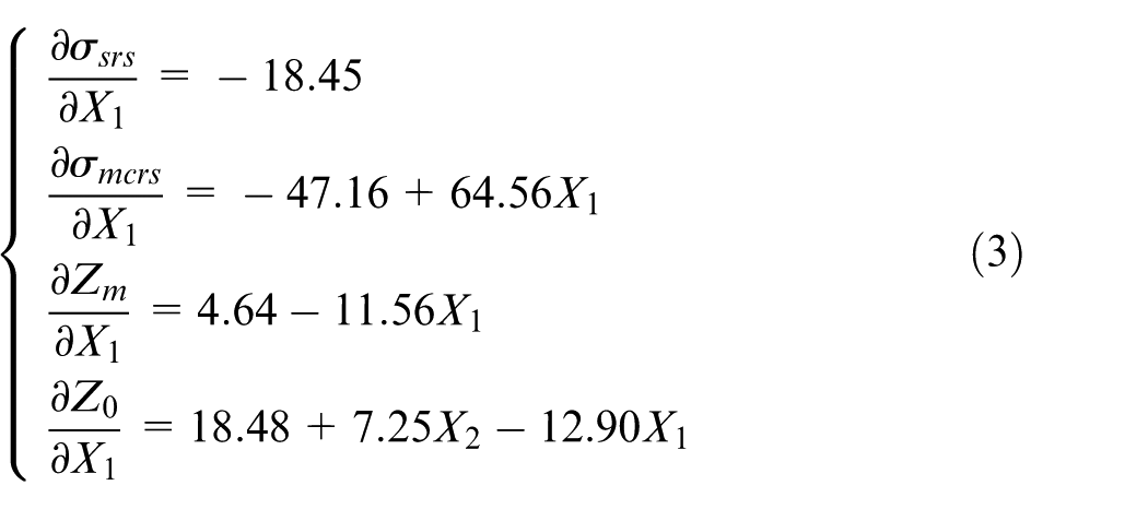
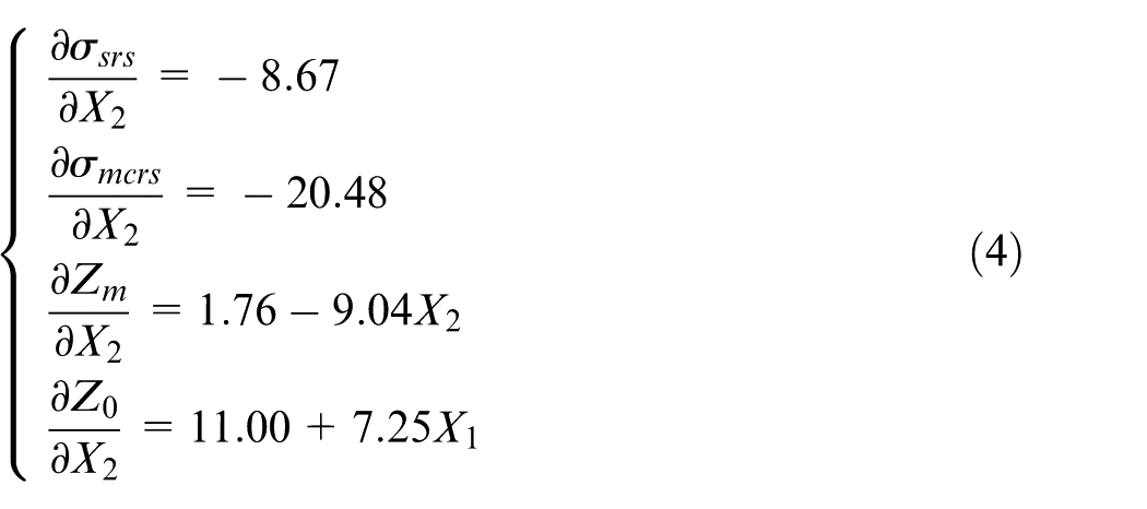
Figure 4 shows the effect of SP parameters on prediction and experimental data of characteristic parameters. Figure 4(a) indicates that as SP intensity increases, the value of σ_srs increases; σ_mcrs, Z_m, and Z₀ increase first and then remain at a certain level. It results from the increase in equivalent static load, and enormous impact energy acts on the material. Thus, the maximum strain will move into the interior of material when it attains saturation at surface. Further increasing the SP intensity, the CRSP can be considered reaching the saturation state. Figure 4(b) shows that the increase in SP coverage causes a significant increase in σ_mcrs and Z₀, while a little change in σ_srs and Z_m. This is probably due to the increase in accumulated plastic deformation and subsequent impact energy. However, when the SP coverage is too large, the plastic deformation of inner metal will restrict Z_m to a deeper location, and the CRSP also reaches a saturation state. From Figure 4, we can also see that the variation magnitude of σ_mcrs and Z₀ was larger than that of σ_srs and Z _m .

Figure 4.

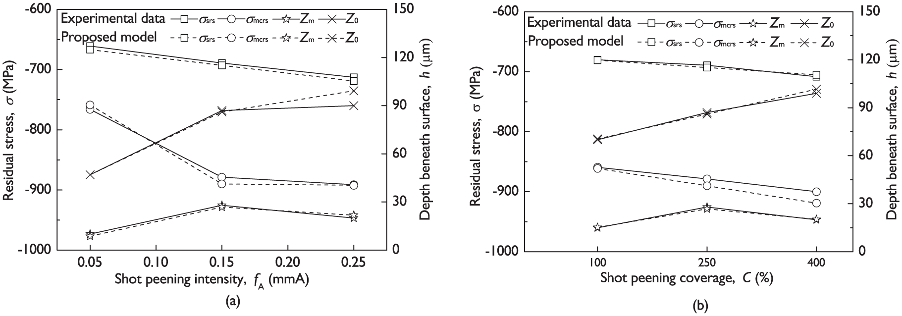
Effect of SP parameters on characteristic parameters: (a) SP intensity and (b) SP coverage.

Sinusoidal decay function model

The obtained CRSPs for 13 different combinations according to Table 4 are shown in Figure 5. Profiles in Figure 5 suggest that the compressive residual stresses increase to a maximum value with an increase in depth beneath the shot-peened surface, and then decrease gradually, eventually remain at the level of residual stress in bulk material. The maximum compressive residual stress occurs at subsurface layer rather than the shot-peened surface, it can be explained by the contact theory of Hertz. ³⁶ The real CRSP results from the combined effect of both competing process, direct plastic surface deformation and plastic deformation of deeper layer due to the Hertz dynamic pressure. When jetting on a hard workpiece with soft shots, the Hertz dynamic pressure is predominant and plastic deformation is weak at surface, resulting shear stress has a maximum value at subsurface. If the maximum shear stress exceeds the flow stress, the plastic elongation will generate maximum compressive residual stress in this depth. When jetting on a soft workpiece with hard shots, the elastic–plastic elongation of the surface is predominant resulting in compressive residual stress with a maximum magnitude at the very surface. In this article, the shot-peened material TC17 alloy is a high-strength material, so Hertzian pressure causes compressive residual stress with a maximum value at the subsurface.

Figure 5.

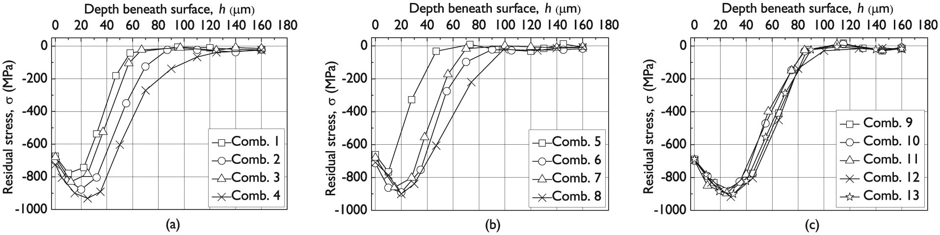
Compressive residual stress profiles measured from the shot-peened surface: (a) Comb. 1–4, (b) Comb. 5–8, and (c) Comb. 9–13.

Residual stress profile has been described using polynomial function of the depth by some researchers.^32,33 The advantage of polynomial fits is the freedom in determination of the number of terms, that is, the order of the polynomial, which can be set to any value up to 1 less than the number of measured points according to the modeler’s subjectivity. Yet the higher the order, the more coefficients of the polynomial should be fitted, thus resulting in low forecasting precision of residual stress profile. Meanwhile, polynomial function may not able to represent the behavior of residual stresses, which reach to a steady value. However, it is observed that the CRSPs resemble the underdamped oscillation of an impulse-loaded spring–mass–damper system, so it is possible to represent the CRSPs using a sinusoidal decay function, which is expressed as shown in equation (5)

$$\mathrm{\sigma }\left(h\right)=A{e}^{-\lambda h}\cos \left({\omega }_{d}h+\theta \right)$$

(5)

where, σ is the residual stress; h is the depth beneath surface; A is the amplitude of underdamped oscillation; λ is the damping coefficient defining how quickly the profile will settle to a steady value; ω_d is the damped frequency which is proportional to the inverse of the period of the profile, and at higher ω_d, the period of the profile gets shorter, representing the sharper peak of CRSP. θ is the phase angle which is ranged between [−π, +π].

The expressions of CRSP using such a function is simple and closed in the form, and the number of coefficients (A, λ, ω_d, and θ) in equation (5) is fixed, which can be named as the controlling factors of CRSP. However, the CRSPs conventionally do not oscillate between positive and negative many times. Therefore, it is proposed here that the CRSPs reach stable state after one decay period. To deduce the model which gives the high fitting precision between the fitted sinusoidal decay function and the measured data, the normalized values of residual stress and depth beneath surface are used. The transformation formula is expressed as shown in equation (6)

$$\{\begin{array}{c}{\sigma }_{normalized}=\left({\sigma }_{actual}-{\sigma }_{min}\right)/\left({\sigma }_{max}-{\sigma }_{min}\right)\\ h_{normalized}=\left(h_{actual}-h_{min}\right)/\left(h_{max}-h_{min}\right)\end{array}$$

(6)

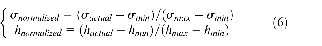
where σ_normalized is the normalized value of compressive residual stress, σ_actual is the actual value of compressive residual stress, σ_min is the minimum value of compressive residual stress which is set to 0 MPa, σ_max is the maximum value of compressive residual stress which is set to −1000 MPa; h_normalized is the normalized value of depth beneath surface, h_actual is the actual value of depth beneath surface, h_min is the minimum value of depth beneath surface which is set to 0 µm, and h_max is the maximum value of depth beneath surface which is set to 160 µm.

The sinusoidal decay function model fitted the experimental data with a high degree of accuracy as shown in Figure 6. This proves the validity of using sinusoidal decay function to fit the CRSPs. The coefficients of A, λ, ω_d, and θ corresponding to the closest fit for different combinations are shown in Table 6.

Figure 6.

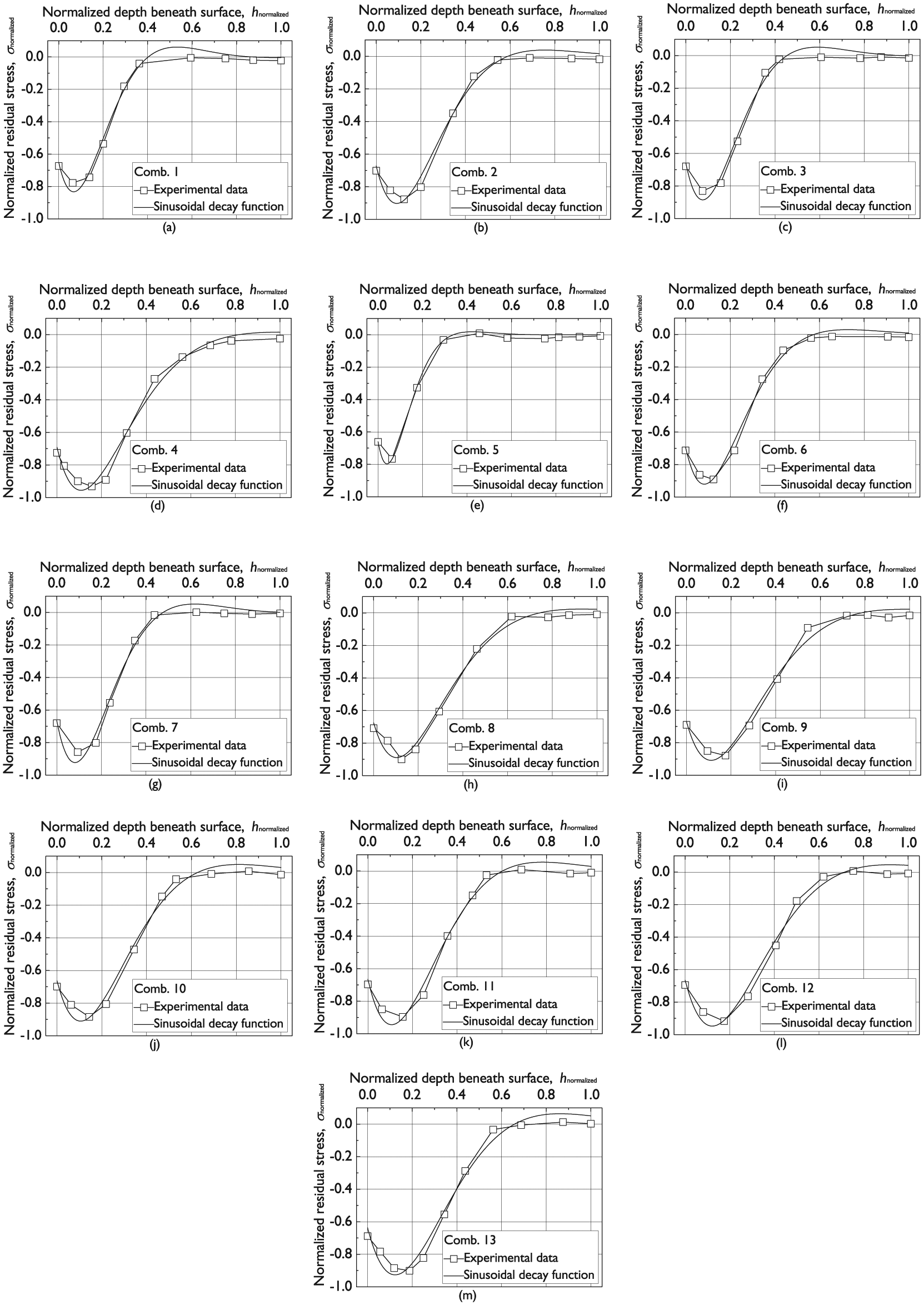
Normalized compressive residual stress profiles measured by experiment and predicted by sinusoidal decay function model: (a)–(m) Comb.1 - Comb.13.

Table 6.

Controlling factors of experimentally determined sinusoidal decay function.

Comb. no.	Controlling factors				Adjusted R2
	A	λ	ωd	θ
1	−1.57780	5.61770	6.74131	−1.1449	0.98355
2	−1.99335	4.78936	4.73826	−1.22674	0.98228
3	−1.81232	5.52433	6.10933	−1.19767	0.98297
4	−2.6194	4.64541	3.51222	−1.3038	0.98307
5	−1.856	9.87512	8.18355	−1.20715	0.99654
6	−2.13827	5.34427	4.88259	−1.24073	0.98733
7	−1.94904	5.39443	5.85824	−1.22279	0.98310
8	−2.13504	4.37784	3.79200	−1.24919	0.98335
9	−2.26794	4.29874	3.61132	−1.27045	0.98159
10	−1.92346	4.13479	4.4452	−1.21868	0.98061
11	−1.99679	4.22004	4.64746	−1.23115	0.98116
12	−2.09655	3.81761	3.93936	−1.24768	0.97830
13	−1.89862	3.61938	4.25319	−1.22848	0.97676

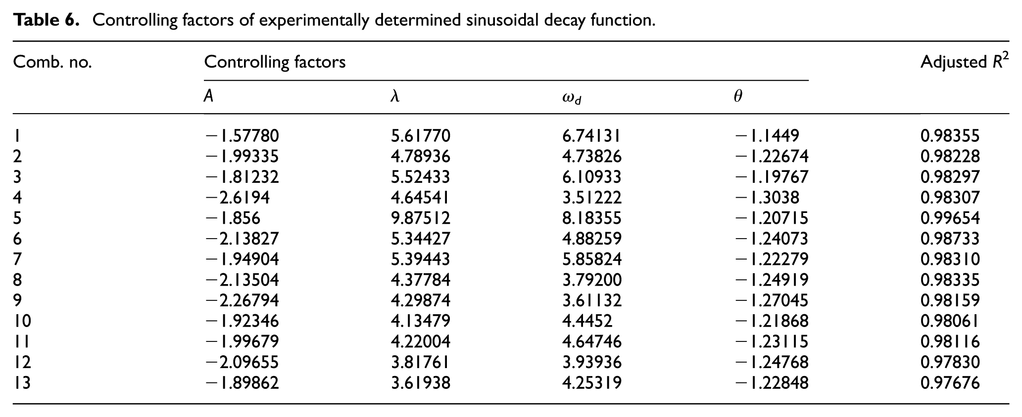
As we know that different SP parameters result in different CRSPs, it is postulated here that the CRSP is a deterministic function of the SP parameters, that is, the controlling factors are individual functions of the two input parameters used. The presumed relation of the controlling factors to SP intensity and coverage is shown in equation (7), where b_ix is the interaction coefficients of SP parameters on controlling factors

$$\left[\begin{array}{c}A\\ \lambda \\ {\omega }_d\\ \theta \end{array}\right]=\left[\begin{array}{cccccc}{b}_{A0}& b_{A{X}_1}& b_{A{X}_2}& b_{A{X}_1{X}_2}& b_{A{X}_1^2}& b_{A{X}_2^2}\\ b_{\lambda 0}& b_{\lambda X_1}& b_{\lambda X_2}& b_{\lambda X_1{X}_2}& b_{\lambda X_1^2}& b_{\lambda X_2^2}\\ b_{{\omega }_{d}0}& b_{{\omega }_d{X}_1}& b_{{\omega }_d{X}_2}& b_{{\omega }_d{X}_1{X}_2}& b_{{\omega }_d{X}_1^2}& b_{{\omega }_d{X}_2^2}\\ b_{\theta 0}& b_{\theta X_1}& b_{\theta X_2}& b_{\theta X_1{X}_2}& b_{\theta X_1^2}& b_{\theta X_2^2}\end{array}\right]\left[\begin{array}{c}1\\ X_1\\ X_2\\ X_1{X}_2\\ X_1^2\\ X_2^2\end{array}\right]$$

(7)

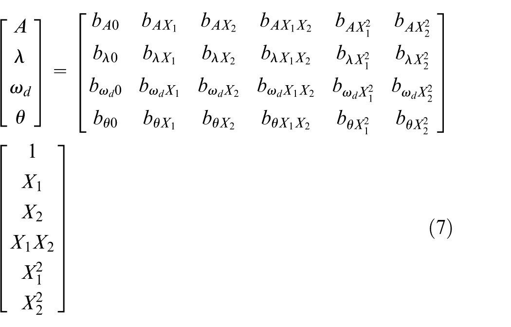
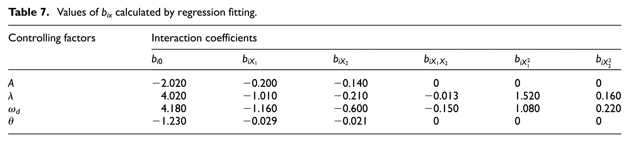
Using the controlling factors of each experiment listed in Table 6, the values of b_ix can be worked out by regression analysis. The calculated values of b_ix are shown in Table 7, which can be used to predict the controlling factors according to any value of f_A and C within the range used in this work. Once the controlling factors are calculated, the CRSP induced by the given SP intensity and coverage is known absolutely. From Table 7, it can be observed that some interactive and quadratic factors are zero, meaning that these factors do not affect the CRSP.

Table 7.

Values of b_ix calculated by regression fitting.

Controlling factors	Interaction coefficients
	$b_{i0}$	$b_{i{X}_1}$	$b_{i{X}_2}$	$b_{i{X}_1{X}_2}$	$b_{i{X}_1^2}$	$b_{i{X}_2^2}$
A	−2.020	−0.200	−0.140	0	0	0
λ	4.020	−1.010	−0.210	−0.013	1.520	0.160
ωd	4.180	−1.160	−0.600	−0.150	1.080	0.220
θ	−1.230	−0.029	−0.021	0	0	0

Verification of the models

To show how the two types of experimental models are used and also to verify the models, two extra tests that were not conducted through the 13 experiments in Table 4 were made. The characteristic parameters and CRSP are predicted and compared with the results of measurement. The specific process is as follows:

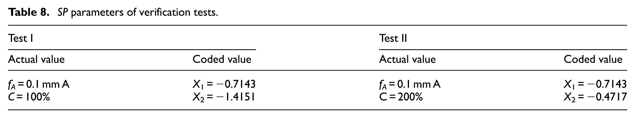
1. Each value of the two input SP parameters should be coded using the transformation equation (1). The actual and coded values of the two extra tests are shown in Table 8.

2. For the characteristic parameters model, the actual values of σ_srs, σ_mcrs, Z_m, and Z₀ can be calculated using equation (2).

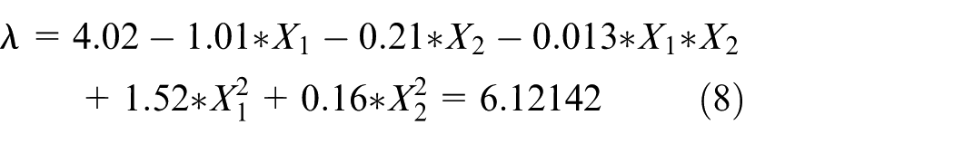
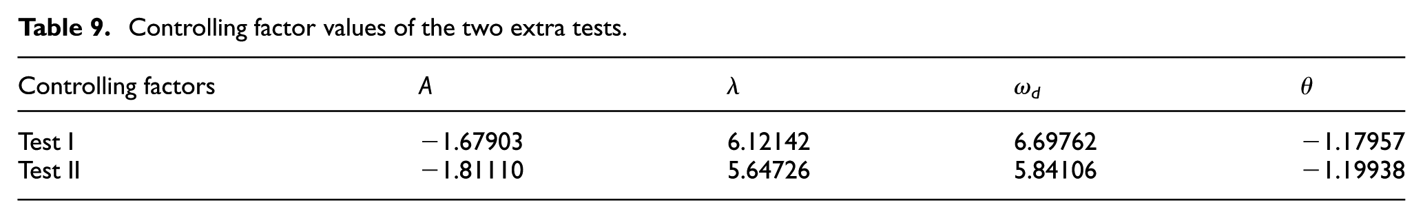
3. For the sinusoidal decay function model, the controlling factors can be calculated using the coded values of the two input parameters and using the b_ix values that are shown in Table 7. For example, the coefficient λ of Test II can be obtained as shown in equation (8). The controlling factor values of the two extra tests are shown in Table 9

   $$\lambda =4.02-1.01*X_1-0.21*X_2-0.013*X_1*X_2+1.52*X_1^2+0.16*X_2^2=6.12142$$
   (8)

4. After obtaining the controlling factor values of the two extra tests, equation (5) that is a function of depth beneath surface, h, could be formed and the normalized CRSP can be determined. By substituting in equation (5) using any value of h_normalized, the σ_normalized at this depth can be obtained. The normalized values of compressive residual stress and depth beneath surface have to be transferred to the actual values using equation (6).

Table 8.

SP parameters of verification tests.

Test I		Test II
Actual value	Coded value	Actual value	Coded value
fA = 0.1 mm A	X1 = −0.7143	fA = 0.1 mm A	X1 = −0.7143
C = 100%	X2 = −1.4151	C = 200%	X2 = −0.4717

Table 9.

Controlling factor values of the two extra tests.

Controlling factors	A	λ	ωd	θ
Test I	−1.67903	6.12142	6.69762	−1.17957
Test II	−1.81110	5.64726	5.84106	−1.19938

The CRSPs predicted by the sinusoidal decay function model as well as obtained by experimental data for the two extra tests are shown in Figure 7. It can generally be observed that the prediction accuracy of the proposed model is preferable. This proves the validity of using the proposed model to predict the distribution of residual stress beneath the shot-peened surface.

Figure 7.

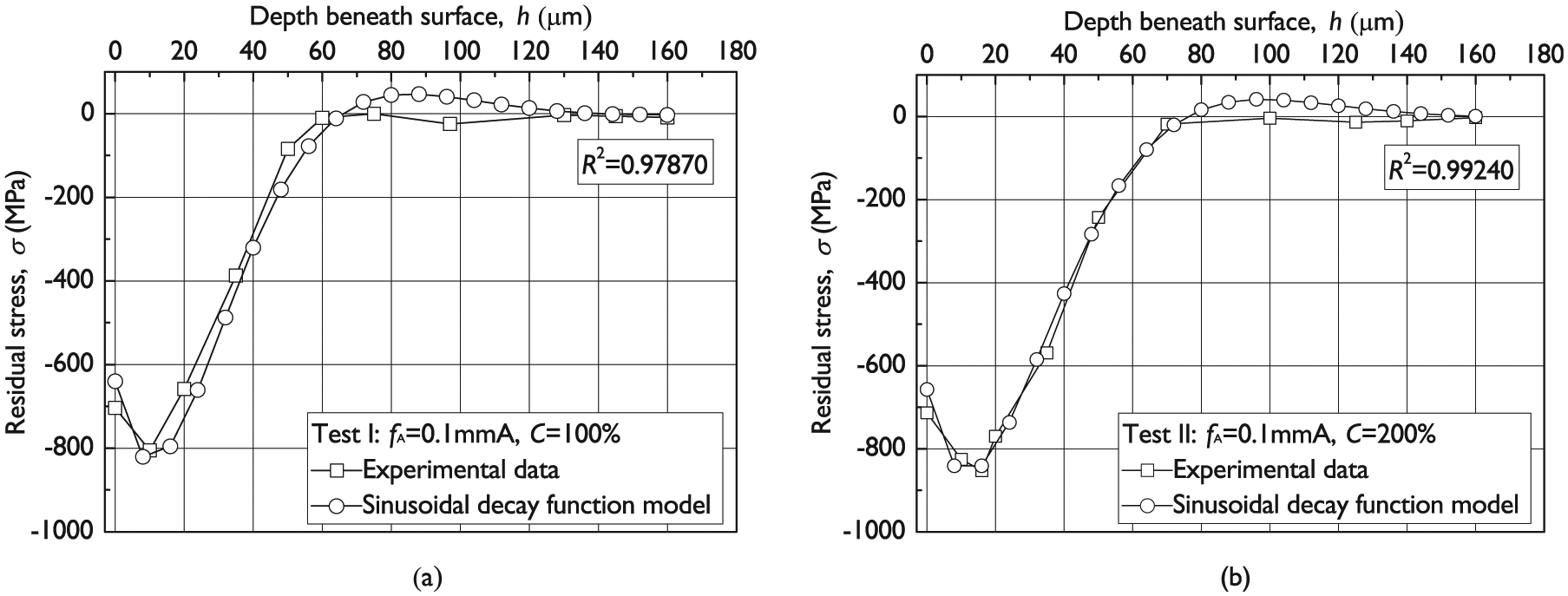
Compressive residual stress profiles measured by experiment and predicted by sinusoidal decay function model: (a) Test I and (b) Test II.

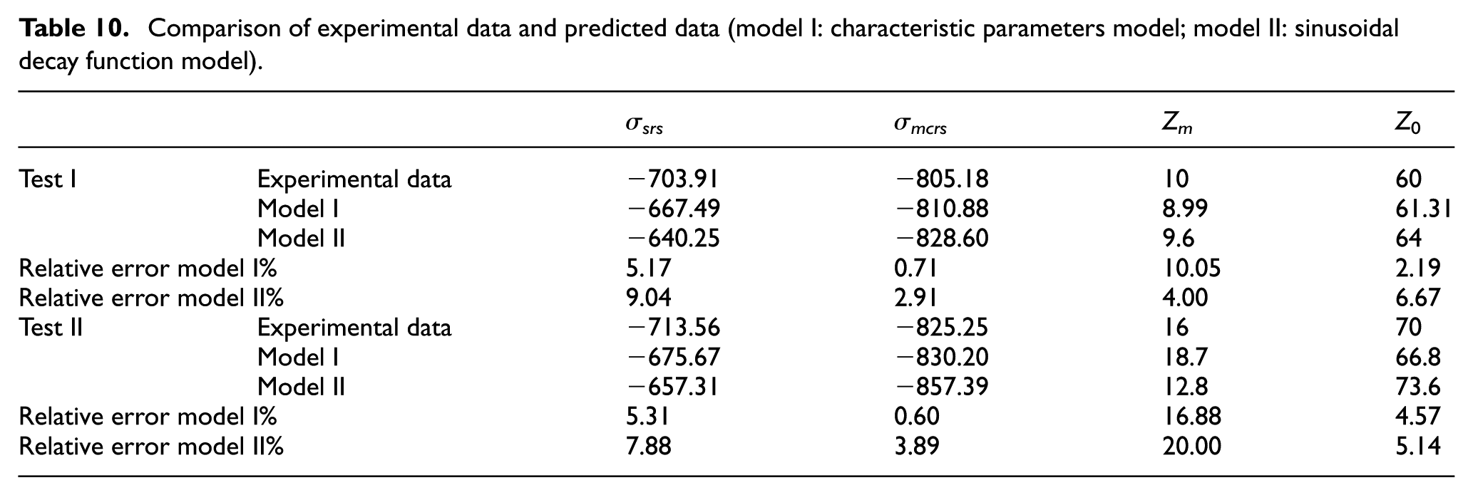
The predicted values of σ_srs, σ_mcrs, Z_m, and Z₀ using the two types of experimental models are shown in Table 10. The predicted values are close to experimental data and the relative errors for all characteristic parameters are less than 20%, meaning that these models can give excellent prediction to characteristic parameters. When comparing the two proposed models, the characteristic parameters model has a higher accuracy of predicting σ_srs, σ_mcrs, Z_m, and Z₀ than the sinusoidal decay function model. However, the characteristic parameters model has been limited to predict the four characteristic parameters; the more comprehensive model of sinusoidal decay function has the capability of predicting CRSP.

Table 10.

Comparison of experimental data and predicted data (model I: characteristic parameters model; model II: sinusoidal decay function model).

		σsrs	σmcrs	Zm	Z 0
Test I	Experimental data	−703.91	−805.18	10	60
	Model I	−667.49	−810.88	8.99	61.31
	Model II	−640.25	−828.60	9.6	64
Relative error model I%		5.17	0.71	10.05	2.19
Relative error model II%		9.04	2.91	4.00	6.67
Test II	Experimental data	−713.56	−825.25	16	70
	Model I	−675.67	−830.20	18.7	66.8
	Model II	−657.31	−857.39	12.8	73.6
Relative error model I%		5.31	0.60	16.88	4.57
Relative error model II%		7.88	3.89	20.00	5.14

Conclusion

This article introduces two experimental models that have the capability of predicting both, the characteristic parameters and the CRSP using two input SP parameters. The contributions of this study are as follows:

1. The characteristic parameters model of predicting the σ_srs, σ_mcrs, Z_m, and Z₀ is established using a response surface methodology which is simple and significant. According to the sensitivity analysis, compared with σ_srs and Z _m , σ_mcrs and Z₀ are more sensitive to the variations of SP parameters. The four characteristic parameters are all more sensitive to the variation of SP intensity than that of SP coverage.

2. The CRSP induced by SP resembles spoon-shaped and the maximum compressive residual stress occurs at the subsurface. As the SP intensity increases, the value of σ_srs increases slightly, while σ_mcrs, Z_m, and Z₀ increase first and then reach a saturation state. The increase in SP coverage causes an increase in σ_mcrs and Z₀, a little change in σ_srs and Z_m.

3. The experimental data of CRSP are fitted using a sinusoidal decay function; the adjusted R² values are greater than 97% for all tests. The relation between CRSP and SP parameters is obtained using regression analysis.

4. The validity of using the two proposed models to predict CRSP is proved by two extra tests, and the prediction errors of all characteristic parameters are less than 20%. The models are very useful to define the SP parameters when a specific residual stress profile is intent, either to help on optimizing the SP parameters.