
Abstract
Bi-rotary milling head is one of the core components of five-axis machining center, and its dynamic characteristics directly affect the machining stability and accuracy. During the sculptured surface machining, the bi-rotary milling head exhibits varying dynamics in various machining postures. To facilitate rapid evaluation of the dynamic behavior of the bi-rotary milling head within the whole workspace, this article presents a method for parametrically establishing dynamic equation at different postures. The rotating and swing shafts are treated as rigid bodies. The varying stiffness of the flexible joints (such as bearings and hirth coupling) affected by gravity and cutting force at different swing angles is analyzed and then a multi-rigid-body dynamic model of the bi-rotary milling head considering the pose-varying joint stiffness is established. The Lagrangian method is employed to deduce the parametric dynamic equation with posture parameters. The static stiffness, natural frequencies and frequency response functions at different postures are simulated using the parametric equation and verified by the impact testing experiments. The theoretical and experimental results show that the dynamics of the bi-rotary milling head vary with the machining postures, and the proposed method can be used for efficient and accurate evaluation of the pose-dependent dynamics at the design stage.
Keywords
Introduction
Bi-rotary milling head with both rotation and swing degrees of freedom (DOFs) is one of the typical configurations of five-axis machine tool and is always used to achieve the machining of large parts with complex surfaces, especially in aerospace industry. In the machining process, many factors affect the machining accuracy such as kinematics errors, thermal errors, dynamic characteristic and tool wear. In the past decades, much research has been focused on the geometric error compensation of five-axis machine tools1–4 and the thermal characteristics of milling head, 5 aiming to improve the machining accuracy.
During the five-axis machining, however, the milling head would change the posture continuously. The different positions and postures may lead to the different static and dynamic characteristics for machine tools. Dhupia et al. 6 performed modal tests on the arch-type reconfigurable machine tool and found the frequency response functions (FRFs) are different from one reconfiguration position (θ = 0°) to another (θ = 45°). Bonnemains et al. 7 and Wu et al. 8 studied the hybrid machine tool and concluded that the static stiffness behaves differently owing to the position variation. Law et al. 9 also found that the natural frequency and dynamic stiffness of the three-axis milling machine behave position dependent. The position-varying dynamics have a great influence on machining stability10,11 and control performance, 12 which limit the achievable productivity and machining trajectories in the whole working range of the machine.
In order to evaluate the varying dynamic behavior at the design stage, some modeling methods have been presented. The most common method is the finite element model (FEM) which is quite convenient to consider the structural flexibility.13–15 But it needs to establish various dynamic models for different configurations and has to be remeshed and recomputed, which is very time-consuming. To improve the modeling efficiency, the co-simulation techniques (CSTs) were proposed to reduce the transition time of modeling from one state to another. One is to integrate FEM and multi-body simulation,16,17 and the other is the integration of FEM and Kriging optimal interpolation. 18 Substructure synthesis technique (SST) was also used to investigate the varying dynamics of machine tools.19–21 In this method, those components are assembled to different configurations of machine tools by small DOFs. Consequently, its computational time and modeling efficiency are improved.
The component flexibility of machine tools can be treated conveniently in the three methods mentioned above, while the contact characteristics between joints or substructures were often ignored. One of the reasons for the varying dynamics of mechanical systems attributes to the variation of the system mass distribution; 22 however, the other is stiffness variation of joints. Cao et al. 23 found that the speed-varying stiffness of bearing joints could lead to speed-varying dynamics of spindles. Yigit and Ulsoy 24 and Dhupia et al. 25 demonstrated that the weakly nonlinear stiffness of machine joints can cause significant variations of natural frequency and dynamic stiffness. The lumped parameter model (LPM), therefore, is proposed to describe the varying dynamics based on varying stiffness of joints. Zhang et al. 26 studied the effect of varying stiffness of kinematic joints with different feed rates on dynamics of the high-speed ball screw system. Wei et al. 27 discussed that the varying joint stiffness of the worm and worm wheel at different tilting angles caused the different dynamics of the tilting table. Wang et al. 28 analyzed the effect of axis coupling force on the stiffness changes of kinematic joints and the varying dynamic behavior of a three-axis gantry milling machine. Comparing to other approaches, LPM is more suitable for the parameterized analysis and reanalysis for the varying dynamics only due to the varying joint stiffness.
FRF at tool center point (TCP) reflects the dynamics of the entire machine tool, and its dominant mode determines the limit cutting depth during cutting process. 29 The machine frame properties can limit FRFs at TCP.30,31 The milling head directly supports the spindle, and its dynamics inevitably affect the dynamic characteristics of TCP. Hung et al. 32 confirmed the influence of the spindle orientation on tool point dynamics and machining stability. Law et al. 33 proposed a dynamic substructuring procedure to model the orientation-dependent dynamic behavior of machine tools with gimbal heads. Yan et al. 34 and Shi et al. 35 also found the variable dynamics of milling head at different postures by FEM. In the modeling process mentioned above,32–35 the joint stiffness was ignored. However, the bi-rotary milling head system contains a large number of joints, such as rotating and swing shaft bearings, hirth coupling and locking joints. Those joints’ stiffness is often less than that of components and some of them vary with different postures. Therefore, to accurately evaluate the varying dynamics of the bi-rotary milling head system at different postures, the joint stiffness has to be considered. This research aims to propose a rapid modeling method to accurately evaluate the dynamic behavior of bi-rotary milling head in the whole working range. A multi-rigid-body dynamic model considering the joint stiffness is established, and the varying stiffness of flexible joints at different postures is analyzed. Finally, a parametric dynamic equation with posture parameters is deduced. Compared with other modeling methods, the pose-varying joint stiffness is considered in the multi-body dynamic model, and the explicit expression of dynamic equation is derived, which can easily and rapidly evaluate the dynamic behavior within the whole workspace.
This article is organized as follows: a dynamic equation with rotation and swing angles is presented in section “Dynamic equation of milling head with rotation and swing angles.” The nonlinear joint stiffness in different machining postures is calculated in section “Calculation of flexible joint stiffness.” The pose-dependent dynamics are analyzed in section “Pose-dependent dynamics.” In section “Experimental verification,” a direct-drive bi-rotary milling head is used to demonstrate the accuracy of the proposed method, followed by conclusions in section “Conclusion.”
Dynamic equation of milling head with rotation and swing angles
Equivalent dynamic model
There are mainly two kinds of bi-rotary milling head, the fork type (Figure 1(a)) and the bias type (Figure 1(b)). The only difference is that the spindle axis overlaps or offsets with the rotation axis.
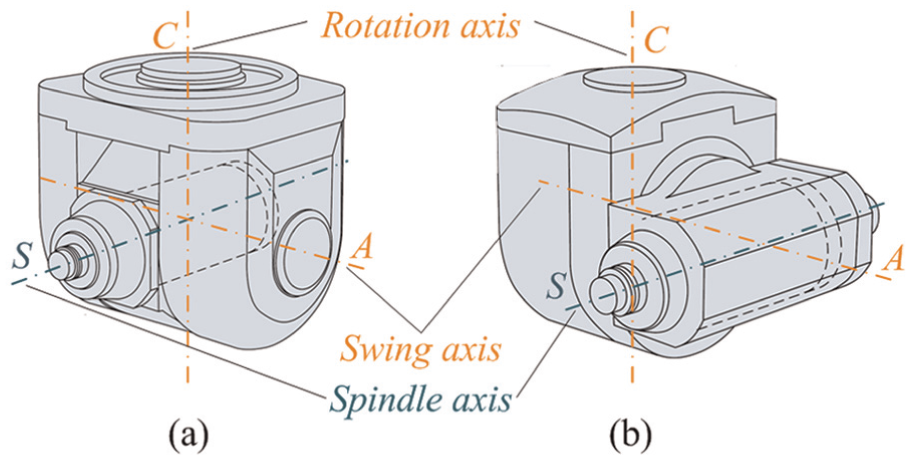
Bi-rotary milling head: (a) the fork type and (b) the bias type.
The fork-type direct-drive milling head considered here generally includes the rotating shaft C-axis, the swing shaft A-axis, A/C-axis drive motors, A/C-axis bearings and A/C-axis locking devices, as shown in Figure 2(a).
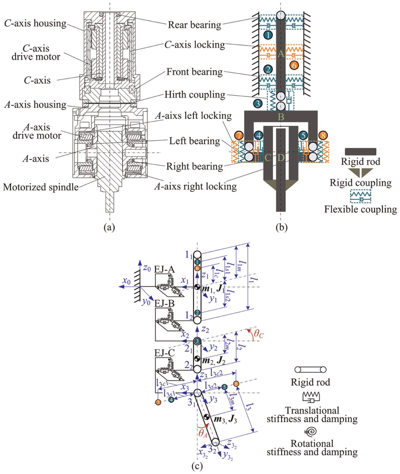
Fork-type bi-rotary milling head: (a) geometric model, (b) dynamic model and (c) calculating model.
Generally, structural stiffness in machine tools is much stiffer than that of the joints and the dominant modes in low frequencies entirely dependent on those flexible joints.28,36 Consequently, for the bi-rotary milling head, the shafts and housings are assumed to be a rigid body due to their larger stiffness at low frequencies, while the bearings are always treated as the flexible coupling. Positioning and locking of A/C-axis in different postures are usually accomplished by mechanical or servo control method. In this case, the stiffness of the locking joints is obviously smaller than that of the shafts, and therefore, they are also considered as the flexible coupling. Although the motorized spindle is a flexible part, it is assumed as a rigid rod and rigidly coupled to the spindle housing for investigating the dynamic characteristics of the bi-rotary milling head itself within the workspace.
Ignoring the motor inductance and all kinds of friction while A/C-axis rotating, we can obtain a multi-body dynamic model for the bi-rotary milling head system, including four rigid rods, eight flexible couplings and one rigid coupling, as shown in Figure 2(b). The four rigid rods are the C-axis (A), A-axis fork housing (B), A-axis (C) and motorized spindle (D), respectively. The eight flexible couplings are listed as the rear bearing (no. 1), front bearing (no. 2), hirth coupling (no. 3), left bearing (no. 4), right bearing (no. 5), C-axis locking joint (no. 6), A-axis left locking joint (no. 7) and A-axis right locking joint (no. 8). One rigid coupling is the connection of the motorized spindle and spindle housing.
The rods A and B are characterized as inertia 1 (
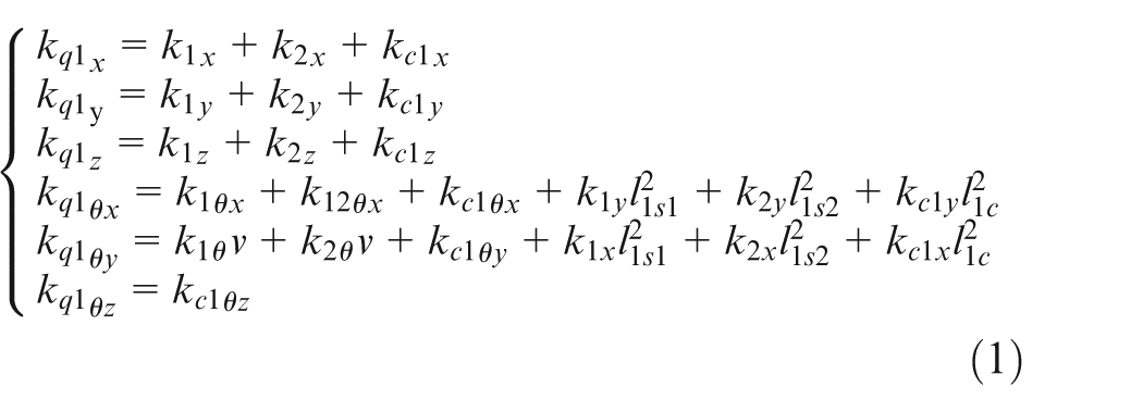
where k1x, k1y, k1z, k1θx and k1θy are the stiffness of the rear bearing, the subscripts x, y, z, θx and θy represent x–y–z translational direction and rotational direction about x- and y-axes (see section “Calculation of flexible joint stiffness”) and similarly hereinafter; k2x, k2y, k2z, k2θx and k2θy are the stiffness of the front bearing; and kc1x, kc1y, kc1z, kc1θx, kc1θy and kc1θz are the stiffness of the C-axis locking joint.
The joint of hirth coupling is defined as EJ-B. Similar to EJ-A, the left bearing, right bearing and left and right locking joints of A-axis are equivalent to EJ-C, with the stiffness written by
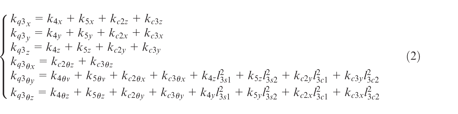
where k4x, k4y, k4z, k4θv and k4θz are the stiffness of the left bearing; k5x, k5y, k5z, k5θv and k5θz are the stiffness of the right bearing; kc2x, kc2y, kc2z, kc2θx, kc2θy and kc2θz are the stiffness of the A-axis left locking joint; and kc3x, kc3y, kc3z, kc3θx, kc3θy and kc3θz are the stiffness of the A-axis right locking joint.
As for the damping of joints, the equivalent process is similar to that of stiffness described above.
Description of the rotation and swing postures
The postures of the rotating and swing shafts can be expressed by an inertial coordinate system fixed on the C-axis housing. Using Cartesian coordinate system, the local coordinate of each rod is shown in Figure 2(c), and its origin is located in the static equilibrium position of gravity and cutting forces. In this figure, θA and θC represent the swing angle and the rotation angle, respectively. The position and posture of each point of the model can be calculated by the coordinate transformation. 37 Set the coordinates of any point P as P(xi, yi, zi) in the moving coordinate system {Oi}, then the coordinates in the relative coordinate system {Oi−1} are calculated by

where
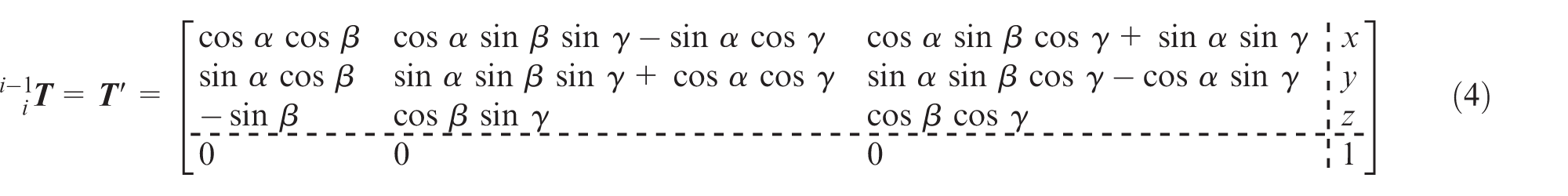
where α, β and γ are the z–y–x Euler angles of the origin of the moving coordinate system in the relative coordinate system; x, y and z represent the position coordinates of the origin of the moving coordinate system in the relative coordinate system.
As the vibration occurs, according to the Maclaurin formula, sin(δα) ≈ δα, cos(δα) ≈ 1 and so on, and
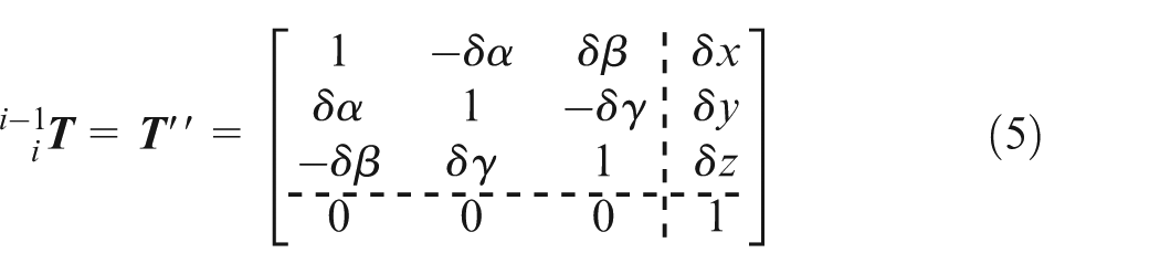
where δα, δβ and δγ are the micro angles of the origin of the moving coordinate system in the relative coordinate system and δx, δy and δz represent the origin’s micro displacements.
By multiplying the transformation matrix of each point, a 4 × 4 transformation matrix of P relative to fixed coordinate system {O0} is
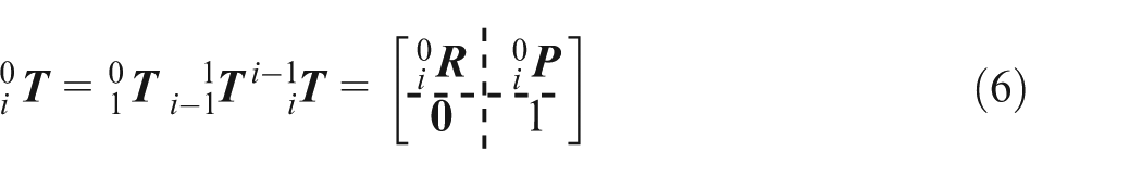
where
As described above, the absolute position and posture of any point of the bi-rotary milling head in the inertial coordinate system can be obtained by the rotation angle, swing angle and geometric parameters. These transformation matrices are included in Appendix 2.
Parametric dynamic equation
Based on the assumption of an ideal constrained system, the system kinetic energy T consisting of the translational kinetic energy and rotational kinetic energy is written as
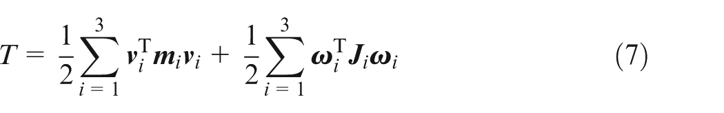
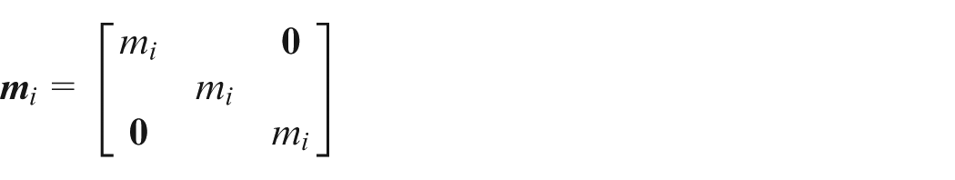
where i is the number of the inertia; the mass matrix of the inertia i is given as
The translational velocity is determined by
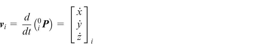
where
The moment of inertia matrix is determined by
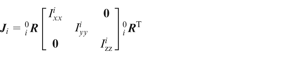
where
The rotational velocity is determined by
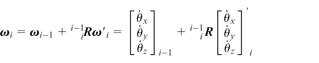
where
Suppose that the system vibrates around the gravity balance position, and consequently only elastic potential energy is left, the potential energy V is expressed as
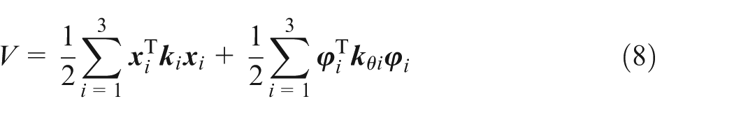
where
The Rayleigh loss function is defined as
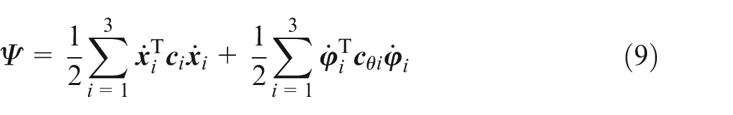
where
Substituting equations (7)–(9) into the Lagrange equation
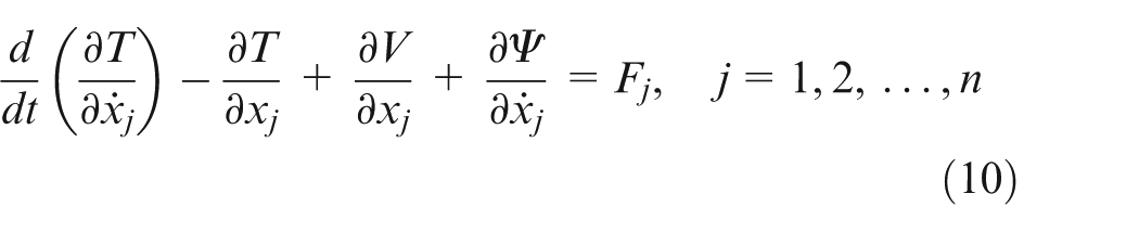
where Fj is the external force in the jth DOF and n is the number of DOF.
We can obtain the dynamic equations of bi-rotary milling head. The centrifugal force and the Coriolis force generated by the rigid-body motion are ignored due to the low rotating and swing speeds. Therefore, linear vibration differential equations are derived in matrix form as

where
As seen from equation (11), the coefficients

where α and β are proportional coefficients.
Finally, substituting equation (12) into equation (11), the pose-dependent dynamic equation of the bi-rotary milling head is expressed as
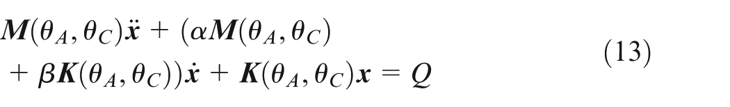
where the mass and stiffness matrices are listed in Appendix 3.
Equation (13) is a second-order linear equation with 18 DOFs. It is convenient to calculate the system pose-dependent dynamics by equation (13) if the posture parameters and physical parameters are known.
Calculation of flexible joint stiffness
Contact stiffness of the rotating shaft bearing
The rotating shaft is usually supported by two bearings: the front one using three-row cylindrical roller slewing bearing is the main load bearing and the rear one using cylindrical roller bearing which is not a load bearing and only radial positioning. Considering the influence of gravity and cutting force, the front bearing loads are written as
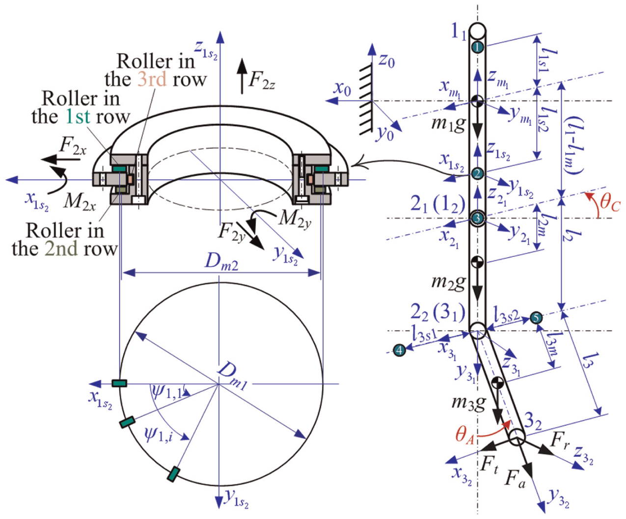
Force diagram of the three-row roller slewing bearing.
The outer ring of the bearing is considered fixed in space as the load is applied to the bearing, and the inner ring could be displaced. The relationship between roller contact deformation and contact force meets Hertz contact deformation. Under the external force vector
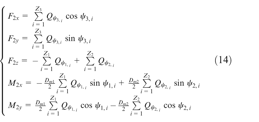
where
The external force vector
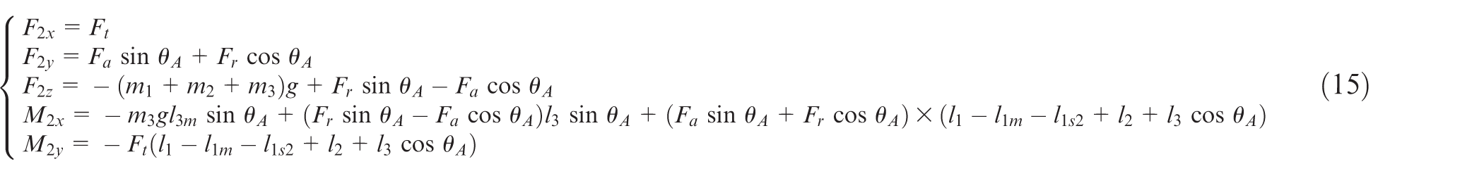
where Ft, Fa and Fr are the three components of average static cutting force, respectively, and g = 9.8 N/kg.
Substituting equation (15) into equation (14), we obtain the relationship of the force vector
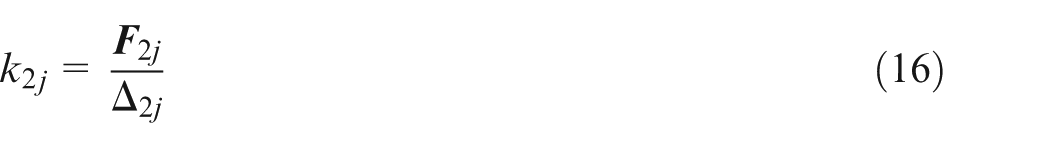
where the subscript j represents the x–y–z–θx–θy deformation direction in turn.
The stiffness of rear bearing which is a general cylindrical roller bearing is calculated directly by the literature. 40
Contact stiffness of the coupling joint for replaceable milling head
For replaceable milling head, the hirth coupling is always used as the coupling between rotating shaft and swing shaft housing, and its loads are noted as
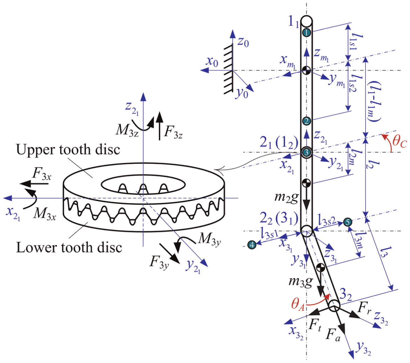
Force diagram of the hirth coupling.
The following assumptions are made: (a) the upper and lower tooth disks of hirth coupling are undeformed except for the contact deformation of the mating surfaces between the upper and lower teeth. (b) The contact between tooth surfaces is uniform. The deformation of centroid of the tooth surface is defined as its overall deformation due to the small area. (c) The radial loads and moments act on the center plane of the hirth coupling. Based on these assumptions, Figure 5 gives the surface contact forces of single tooth as well as the definition of coordinate system.
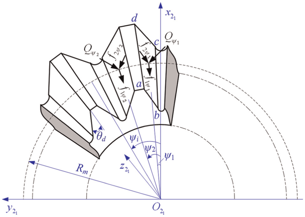
Force diagram of tooth surfaces of the hirth coupling.
The position angle of each pair of mating teeth surfaces is determined by
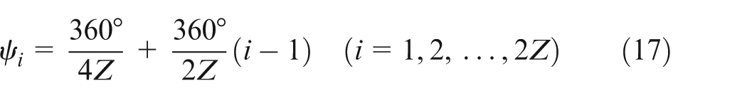
where Z is the number of teeth.
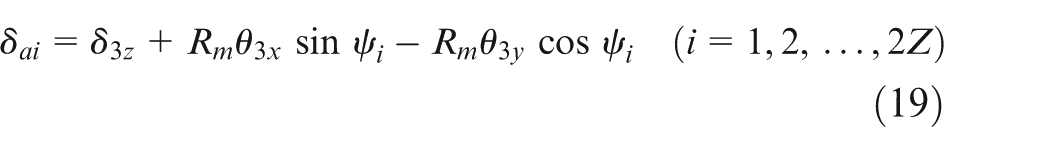
Supposing the upper tooth disk is constrained, the lower tooth disk would produce a displacement Δ3 described as Δ3 = {δ3x, δ3y, δ3z, θ3x, θ3y, θ3z} under the external load
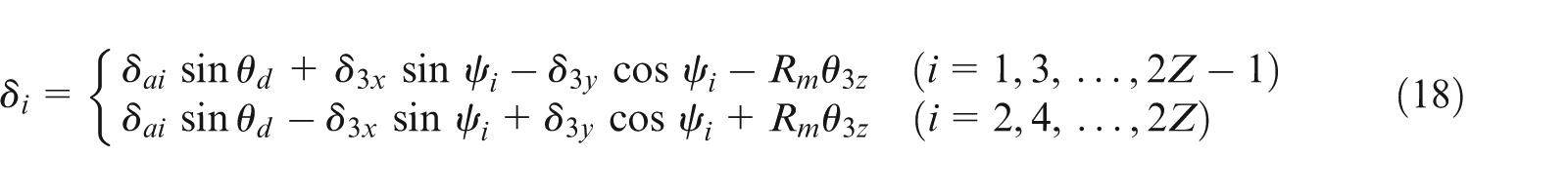
where θd is the pressure angle of the mating surface, Rm is the circle radius of the mating surface centroid and δai is given by
For the single tooth surface, the relationship between elastic deformation δ and the average surface pressure Pn can be expressed as41,42

where a and b are constants determined by machining methods, materials and so on.
Substituting equations (18) and (19) into equation (20), we obtain the normal contact load of each pair of the mating tooth surfaces
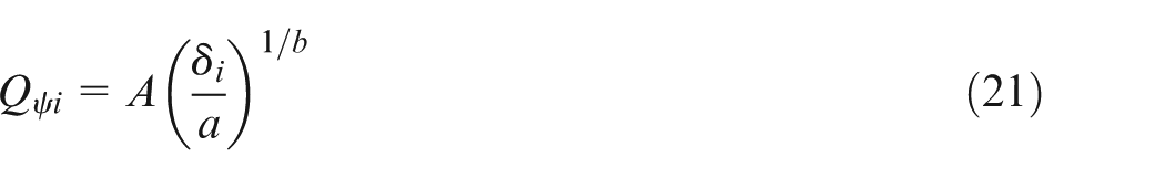
where A is the contact area.
The force and moment balance equations of hirth coupling are established as
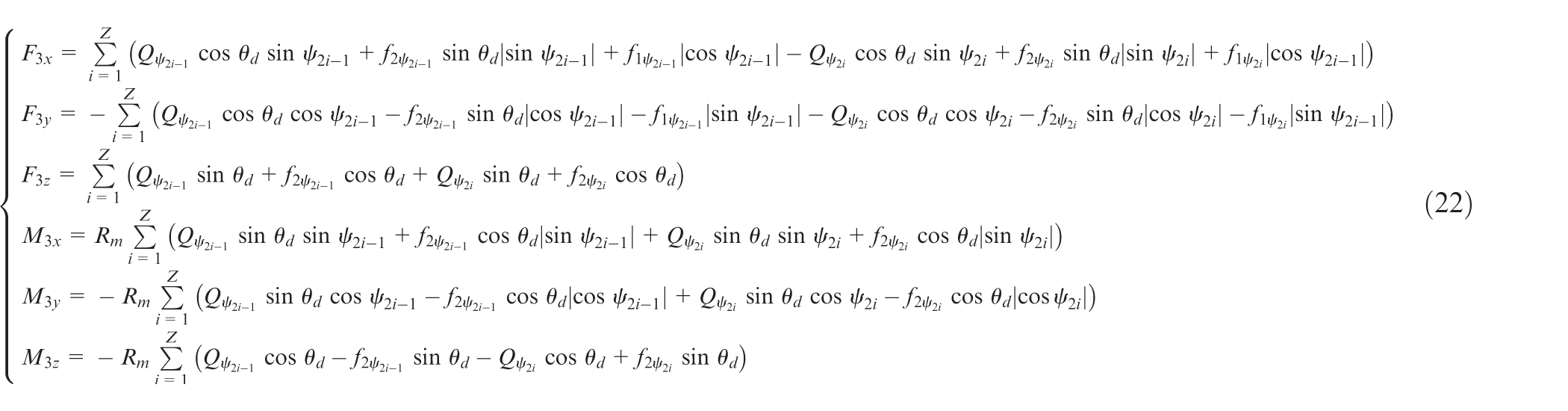
where
The external force vector is
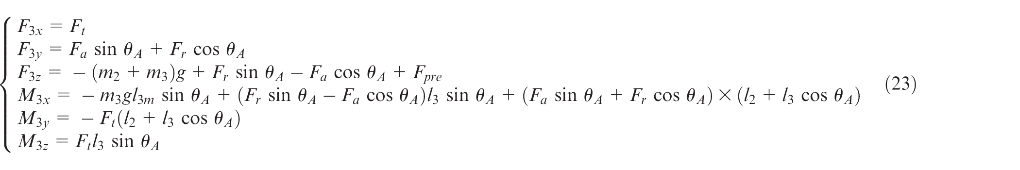
where Fpre is the initial preload.
The least square fitting method or Newton–Raphson method can be employed to calculate the deformation Δ3 through equations (17)–(23) and then the contact stiffness is given by
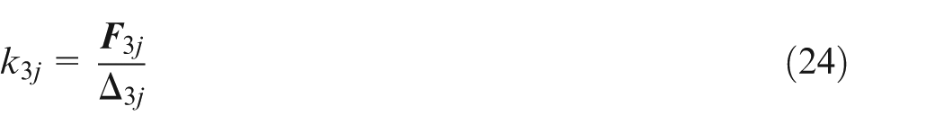
where the subscript j represents the x–y–z–θx–θy–θz deformation direction in turn.
Contact stiffness of the swing shaft bearing
Cross-roller bearing is always used to support the swing shaft. Affected by the gravity, cutting force and swing posture, the bearing is also loaded by a 5-DOF external force
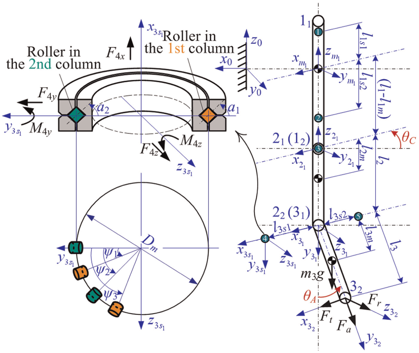
Force diagram of the cross-roller bearing.
Assuming that the outer ring of the bearing is fixed, then the inner ring produces a displacement as the load is applied to the bearing. The relationship between roller contact deformation and contact force meets Hertz contact deformation. The force and moment balance equations of bearing are as follows 43
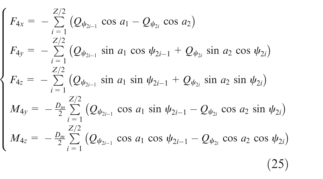
where
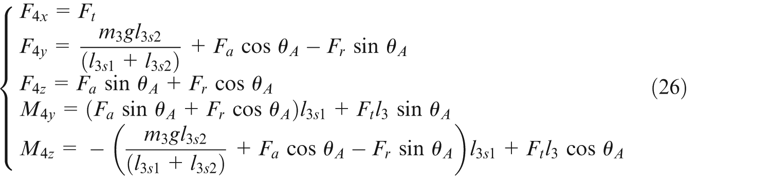
Substituting equation (26) into equation (25), we can establish the relationship of the force vector
where the subscript j represents the x–y–z–θy–θz deformation direction in turn.
Contact stiffness of the locking joint
As mentioned above, two methods are commonly used for the positioning and locking of the rotating and swing shafts. Considering the fixed angle machining, the mechanical method is discussed here, and it is achieved by the friction of contact surface between the friction ring and the shaft, as shown in Figure 7(a). The contact surface (Sabcd) is cylindrical, as shown in Figure 7(b).
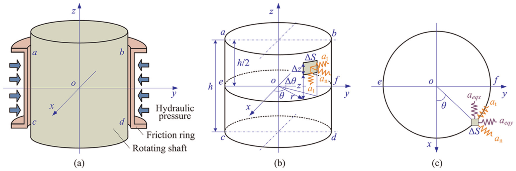
Schematic diagram of cylindrical locking joint: (a) operating diagram, (b) structure diagram and (c) schematic diagram of xoy plane.
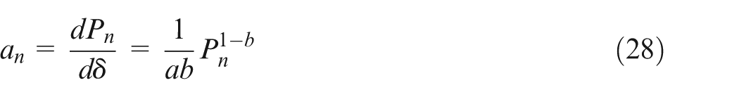
It is assumed that the contact surface of the friction ring is uniformly pressured. For cylindrical contact surface per unit area (ΔS: r × Δθ × Δz), three orthogonal contact stiffness are considered including one normal contact stiffness an and two tangential stiffness at, respectively. From equation (20), taking the derivative of Pn with respect to δ we can yield
The relationship between tangential contact stiffness and normal contact stiffness is 44

where αnt is constant determined by materials, surface roughness and so on.
As shown in Figure 7(c), the normal and tangential contact stiffness can be transferred to the values in the Cartesian coordinates {Oxyz}, expressed as
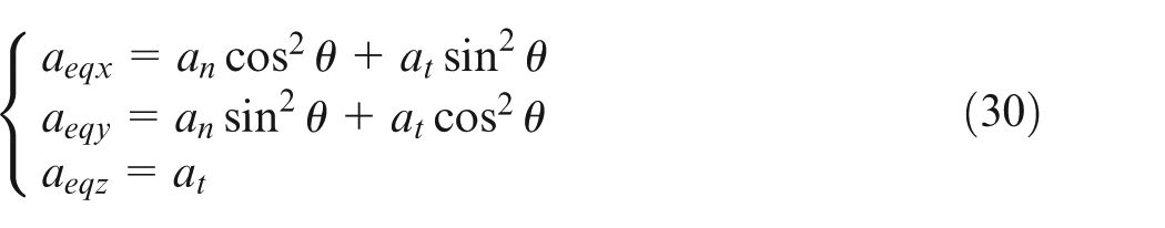
where θ is the position angle in the circumferential direction.
Finally, integrating in the whole contact surface, we can obtain the total contact stiffness of the cylindrical joint as follows
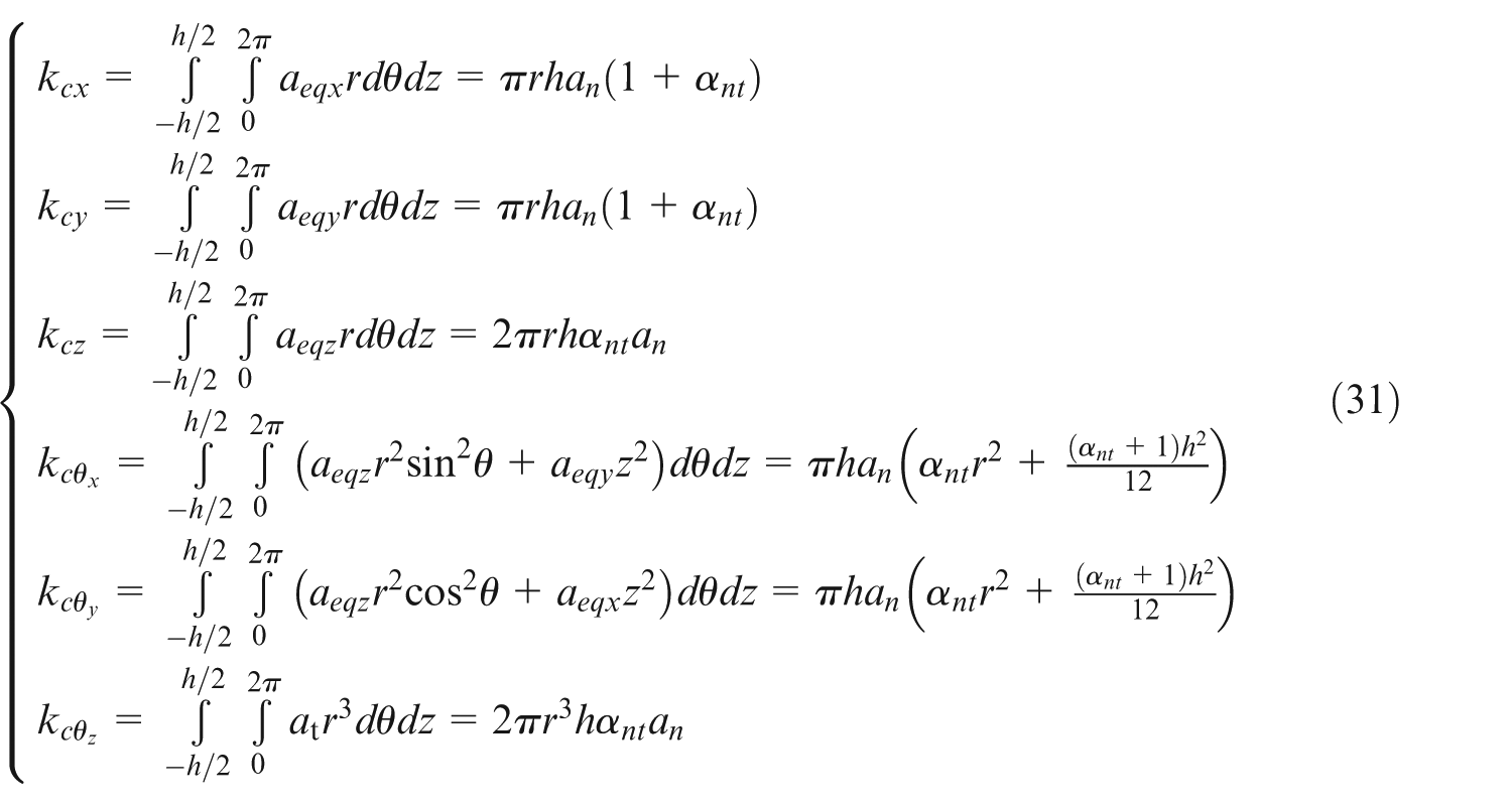
where h and r are the height and radius of the cylindrical joint, respectively.
Substituting the parameters of A/C-axis locking joint into equation (31), we can obtain the stiffness of the C-axis locking joint
Pose-dependent dynamics
Static stiffness at different postures
The dynamics of a bi-rotary milling head shown in Figure 2 within its workspace were calculated by the parametric equation (13). The simulation parameters are included in Appendix 4. The static stiffness maps of the milling head at the spindle nose is shown in Figure 8, where it can be seen that the translational and rotational stiffness are symmetric about θA = 0°. The values of Kx, Ky, Kθx and Kθz reach the minimum at θA = 0°, while their maximum are at θA = 90°. But the minimum and maximum values of Kz and Kθy are opposite.
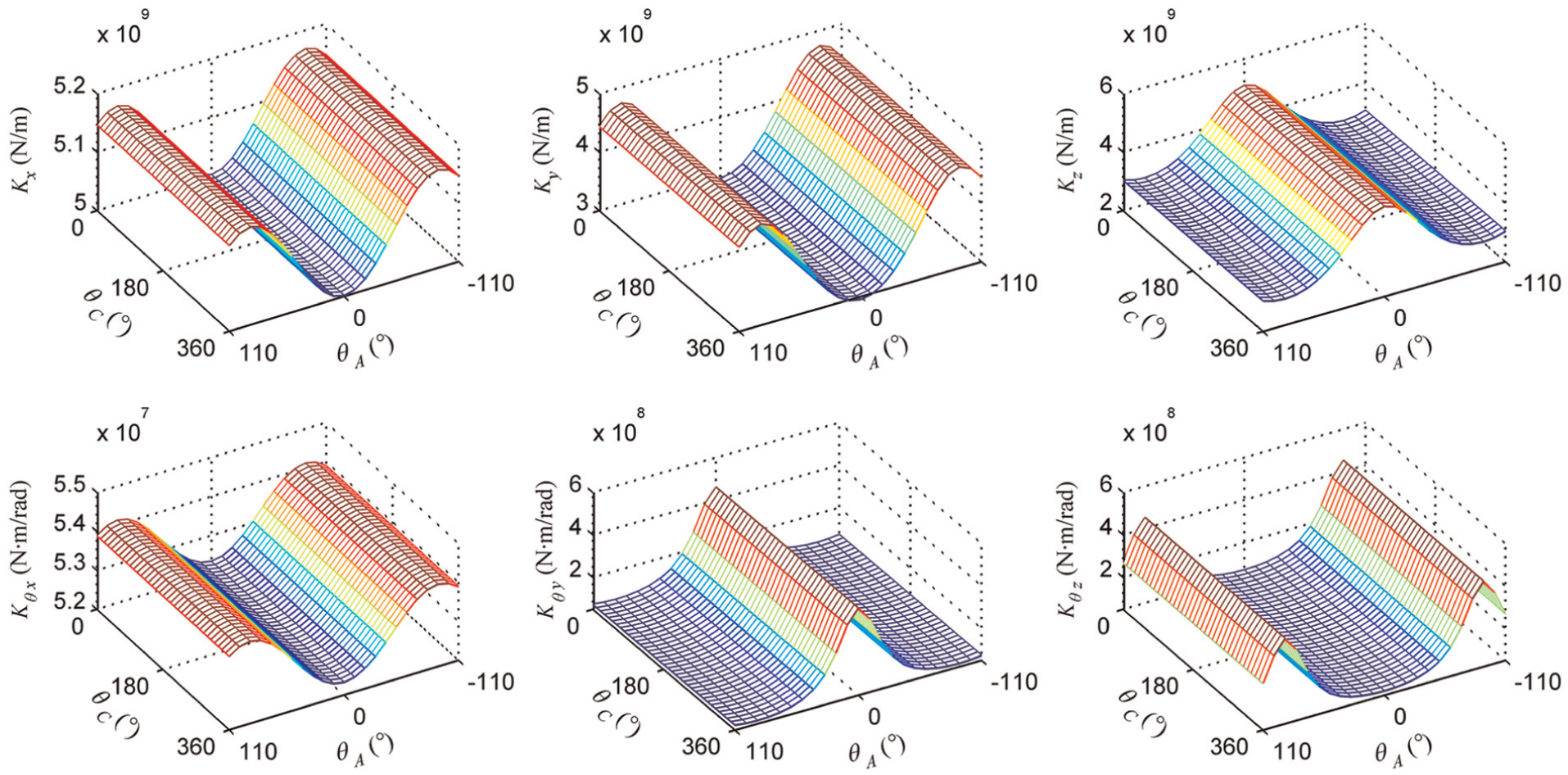
Static stiffness maps at the spindle nose.
Natural frequencies at different postures
Figure 9 shows the variation of natural frequencies during the whole working postures. As it can be seen, the rotation angle has little effect on the system natural frequencies, and the first two natural frequencies at positive and negative swing angles are almost the same due to the structural symmetry. However, it is a remarkable fact that the two natural frequencies both increase with θA.
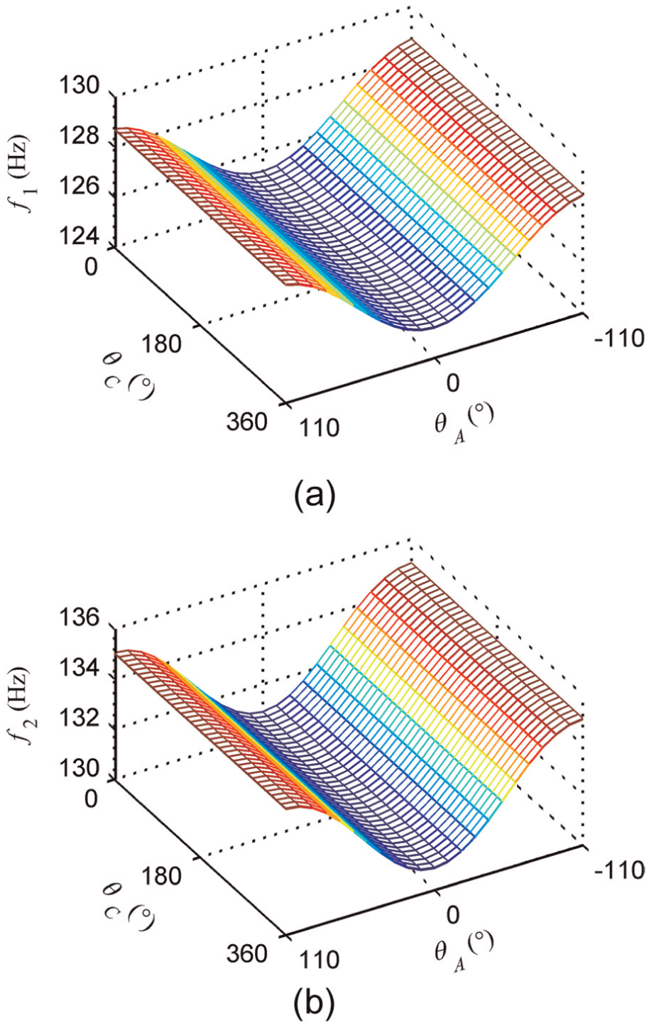
Pose-dependent natural frequencies of the bi-rotary milling head: (a) first natural frequency and (b) second natural frequency.
FRFs at different swing angles
The FRFs at the spindle nose within swing angles from 0° to 90° are shown in Figure 10. The first and second natural frequencies increase with the swing angle which is consistent with the discussion in the previous section. The amplitude at the first natural frequency slowly increases with θA; however, the amplitude at the second natural frequency decreases significantly with the increase in θA.
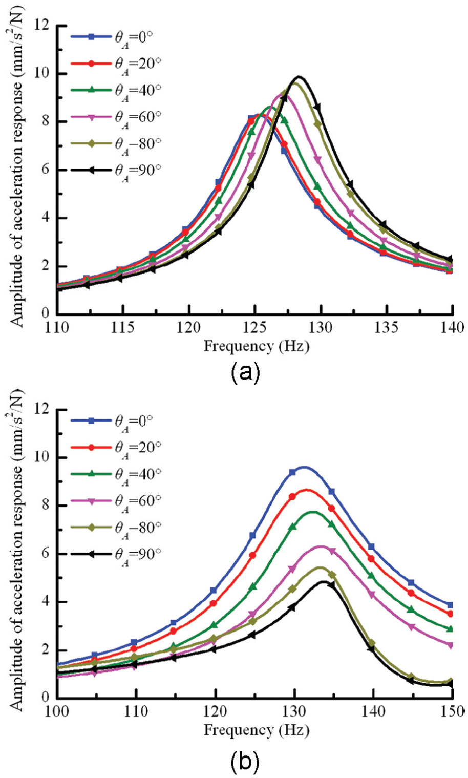
FRFs of simulation at the spindle nose at different swing angles: (a) YY FRFs and (b) XX FRFs.
Reasons for pose-dependent dynamics
From Figures 8–10, the dynamics of the bi-rotary milling head are pose dependent and sensitive to the swing angle. The variation of the swing angle can change the system moments of inertia according to equation (13), thereby changing its mass matrix, as shown in Figure 11. Moreover, the stiffness matrix is also changed owing to the nonlinear change of flexible joints at different swing angles.
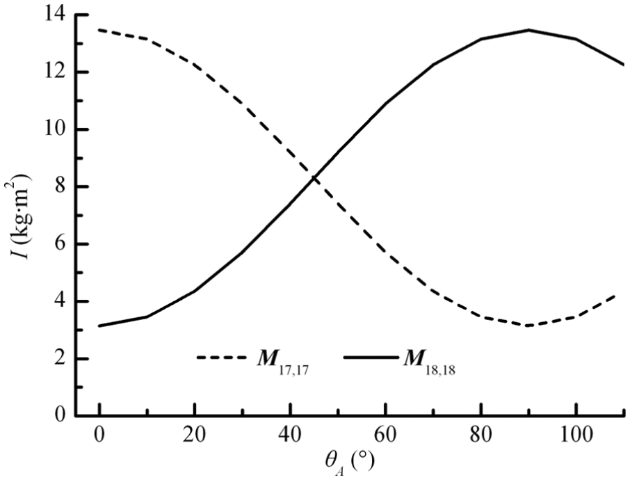
Influence of the swing angle on the mass matrix.
The eccentric mass m3 would produce a moment M2x which can be calculated by equation (15) when the swing shaft swings without other loads, as plotted in Figure 12. It can be clearly seen that the gravity moment varies with the swing angle. Subjected to the varying moment, the equivalent contact stiffness of the front bearing at different swing angles is calculated by equations (14)–(16), as shown in Figure 13(a). It indicates that k2θx varies obviously with the swing angle. For the joint of the hirth coupling, as shown in Figure 13(b), the contact stiffness calculated by equations (17)–(24) is also varying.
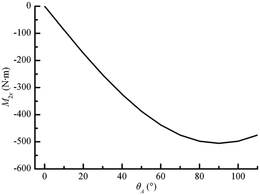
Variation of gravity moment with the swing angle.
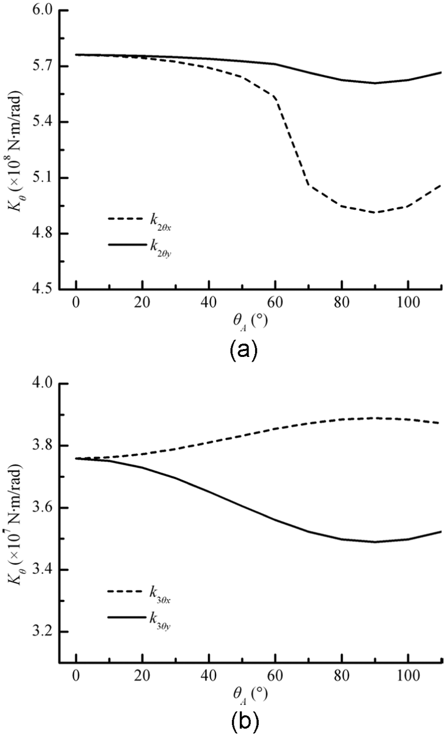
Influence of the swing angle on the contact stiffness: (a) the joint of three-row cylindrical roller bearings and (b) the joint of hirth coupling.
Figure 14 describes the influence of the varying moment of inertia and stiffness on natural frequencies with the swing angle. For the first natural frequency, plotted in Figure 14(a), the change of mass matrix Δ
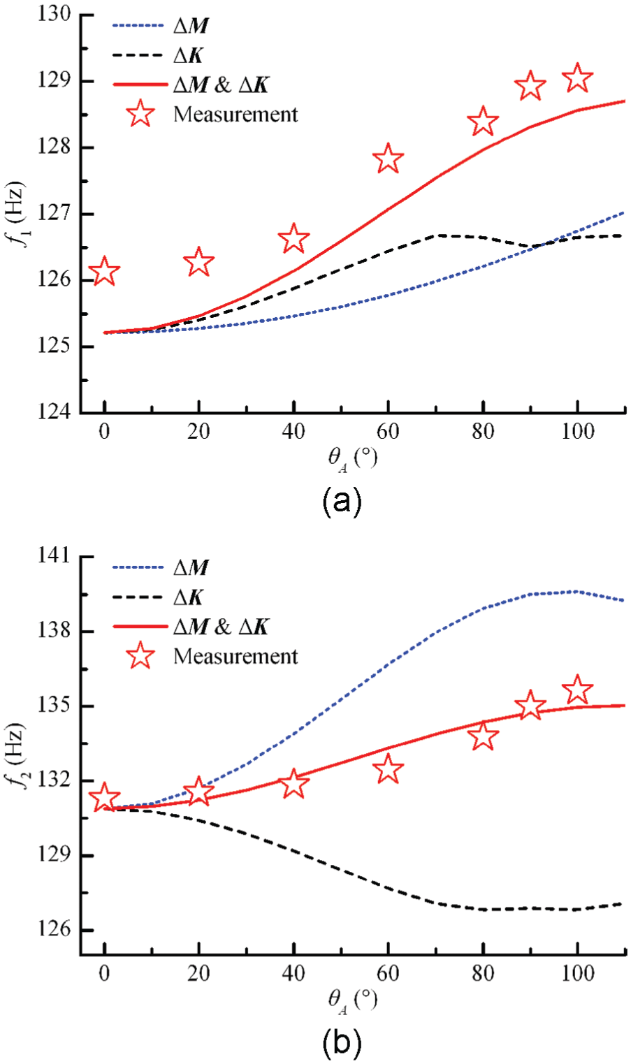
Influence of the swing angle on the natural frequency: (a) first natural frequency and (b) second natural frequency.
Experimental verification
Experimental setup
A fork-type direct-drive bi-rotary milling head with A/C-axis (θA ∈ −110° to 110°; θC ∈ 0°–360°) was employed as the test object, as shown in Figure 15, where the front bearing adopts three-row roller slewing bearing (model: YRT 325), the rear one is cylindrical roller bearing (model: N 1922) and both the left and the right bearings use cross-roller bearings (model: SX 011824) with a supporting span of 368 mm. The circumferential hydraulic brake with a pressure of 4 MPa is used for the locking of A/C-axis. The maximum torque and the highest speed of C-axis motor are 2394 N m and 60 r/min, while for A-axis motor, the values are 1450 N m and 60 r/min, respectively.
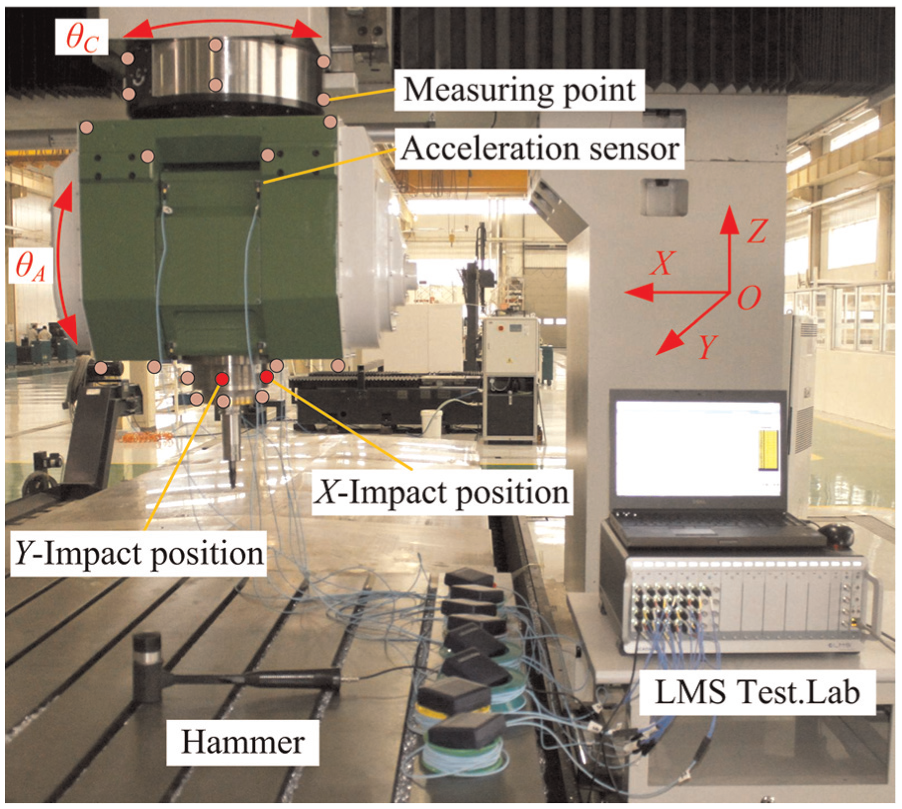
Impact testing experiment.
Modal testing was performed by LMS Test.Lab with a hammer (model: PCB 086D05, sensitivity: 0.21 mV/N) exciting on the spindle nose and three-direction acceleration sensors (model: PCB 352A16, sensitivity: 100 mV/g) used to pick acceleration response of the measuring points distributed on the milling head. The number of measurement points is 40, the frequency bandwidth is 512 Hz and the number of spectral line is 2048. And then the modal frequencies, mode shapes and FRFs were calculated by model analysis module of the test system. The tests were repeated every 20° within swing angles from 0° to 100°.
Comparison between experimental and simulated results
Test results of natural frequencies at different swing angles are plotted in Figure 14. The first two natural frequencies both increase with the swing angle, and the variation is consistent with the evaluated results. Moreover, the evaluated value at each swing angle is very close to the experimental value. The mode shape of the first frequency is a first-order swing mode around the x-axis (Figure 16(a)), and the second mode shape is a first-order swing mode around the y-axis (Figure 16(b)). Figure 16 shows that the low-frequency modes of the milling head are the relative vibration between structural components, so the rigid-body assumption is tenable.
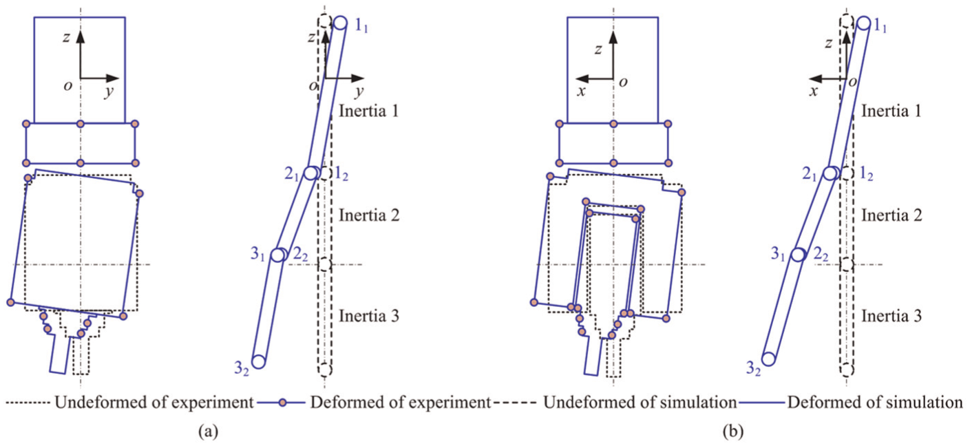
Mode shape comparison between experimental and simulated results: (a) first mode (126 Hz) and (b) second mode (131 Hz).
The measured FRFs at different swing angles are shown in Figure 17. The change trend of the first two natural frequencies and corresponding amplitudes are also close to the evaluated values (Figure 10) although there exists a little discrepancy at the swing angles of 80° and 90°. The different amplitudes at the resonance peaks between the simulation and the experiment are mainly affected by the damping. The Rayleigh viscous equivalent damping is used in the model, while the damping of the actual system is a nonviscous damping. In addition, the residual modes and the neglect of the cross stiffness of the joint are also the factors causing the error. Compared with the tested natural frequencies and FRFs, the simulated results can match well with the experimental results, which validate the modeling method proposed above.
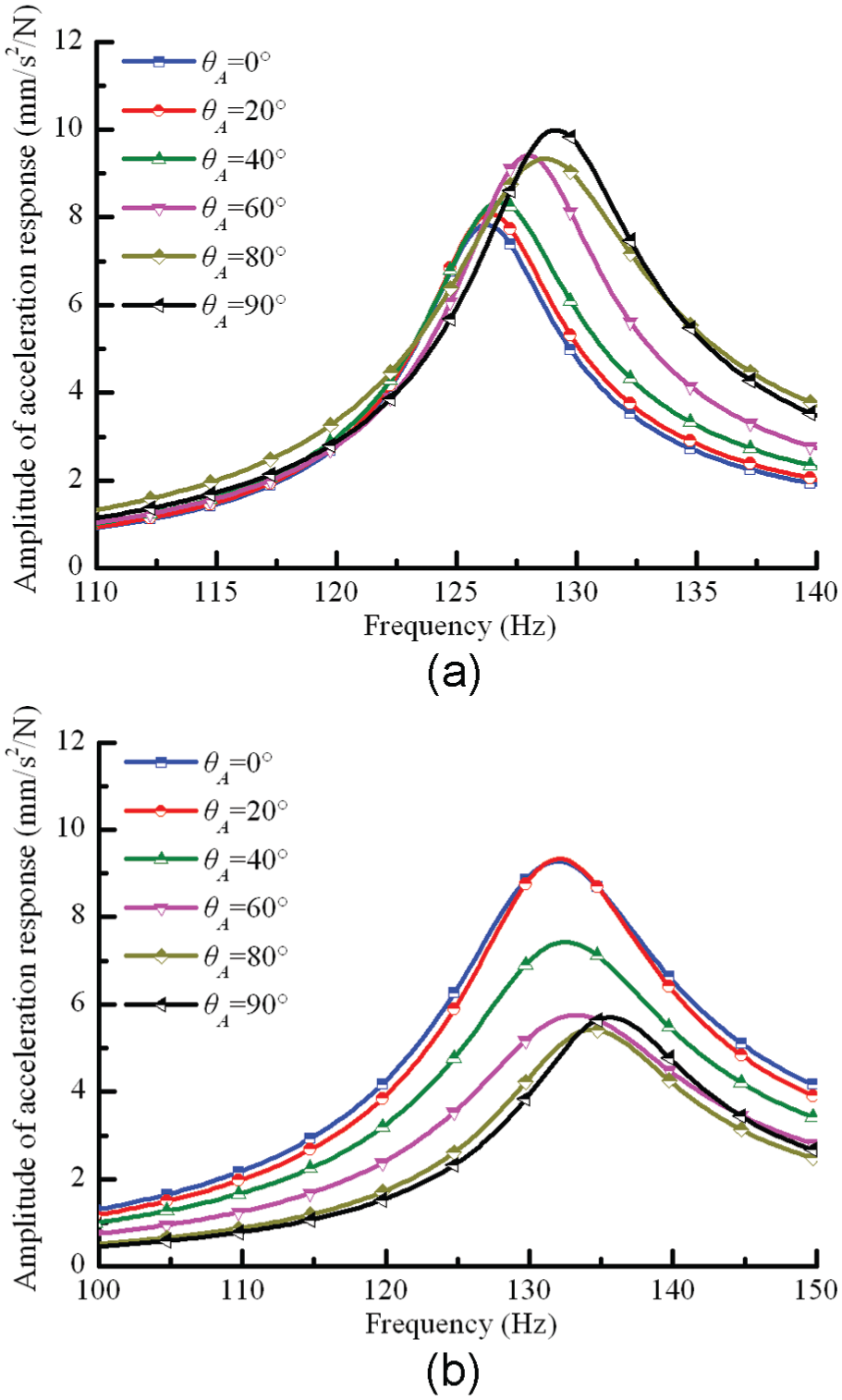
FRFs of experiment at the spindle nose at different swing angles: (a) YY FRFs and (b) XX FRFs.
Conclusion
In this article, a parametric modeling method is presented to evaluate the pose-dependent dynamics of bi-rotary milling heads. The explicit expressions of the system mass, damping and stiffness matrices with rotation and swing angles are obtained in a straightforward way, which is conducive to elegant and efficient simulation and analysis of the dynamic behavior within the whole workspace. Moreover, the pose-varying stiffness of joints is considered. Using this method, a fork-type direct-drive bi-rotary milling head is analyzed, and the main conclusions are as follows:
The predicted and measured results indicate that the system dynamics are pose dependent in terms of static stiffness maps, natural frequencies and FRFs at different postures. The reasons are not only the variation of the mass distribution of the system but also the varying stiffness of three-row cylindrical roller slewing bearing and hirth coupling affected by the gravity at different swing angles.
The pose-dependent dynamics are sensitive to the swing angle while nonsensitive to the rotation angle. It is because that the rotating angle does not change the relative position between the rotating shaft and swing shaft, and the joint stiffness is a constant at a certain swing angle.
The parametric modeling method can also be used for other milling heads with different structures and transmission forms to facilitate rapid assessment of design alternatives at an early stage of development. Furthermore, the dynamic model of tool–spindle–milling head system can be established, which helps to explore the effect of pose-dependent dynamics of the milling head on cutting stability to improve machining accuracy and efficiency of five-axis machine tools.
Footnotes
Appendix 1
Appendix 2
Transformation matrix of each point on the bi-rotary milling head.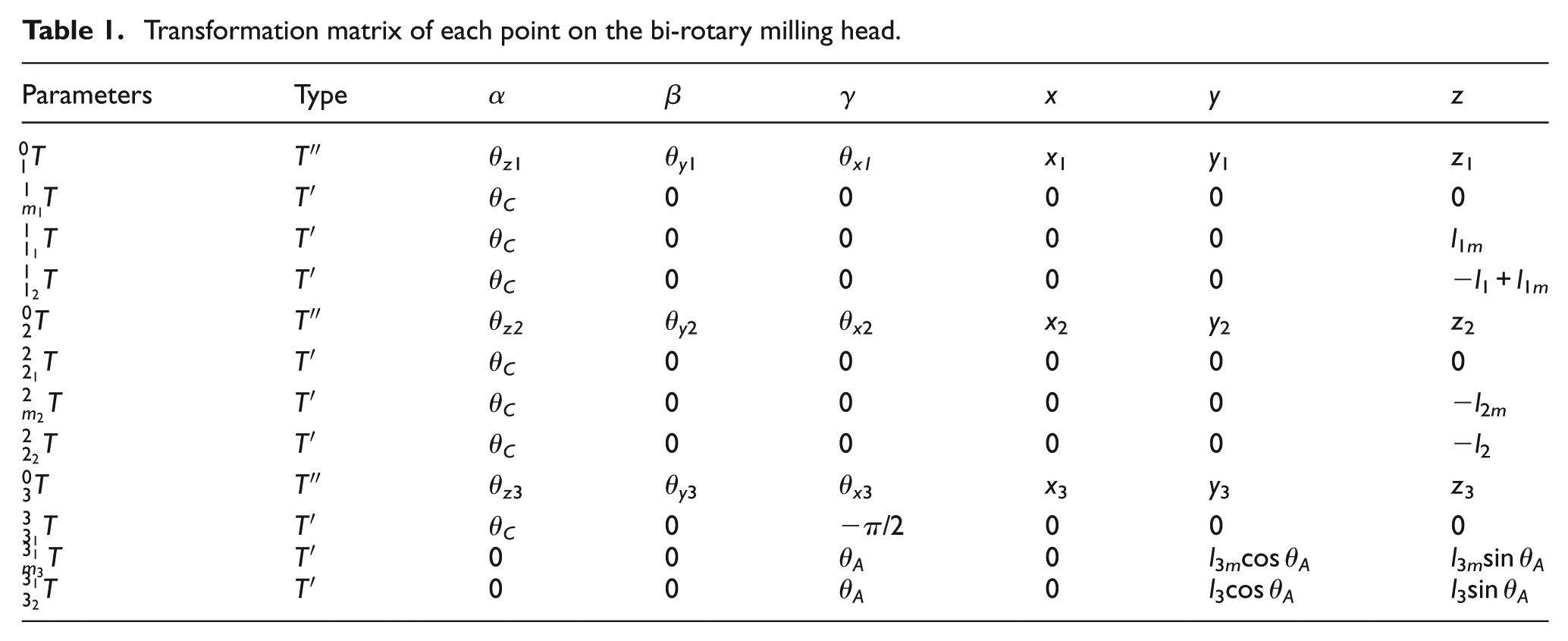
Parameters
Type
α
β
γ
x
y
z
θz
1
θy
1
θx1
x
1
y
1
z
1
θC
0
0
0
0
0
θC
0
0
0
0
l
1m
θC
0
0
0
0
−l1+l1m
θz2
θy
2
θx
2
x
2
y
2
z
2
θC
0
0
0
0
0
θC
0
0
0
0
−l2m
θC
0
0
0
0
−l2
θz
3
θy
3
θx
3
x
3
y
3
z
3
θC
0
−π/2
0
0
0
0
0
θA
0
l3mcos θA
l3msin θA
0
0
θA
0
l3cos θA
l3sin θA
Appendix 3
The system mass matrix
where
The system stiffness matrix
where
Appendix 4
Parameters for the dynamic model of the bi-rotary milling head are presented in the following.
Declaration of conflicting interests
The author(s) declared no potential conflicts of interest with respect to the research, authorship and/or publication of this article.
Funding
The author(s) disclosed receipt of the following financial support for the research, authorship, and/or publication of this article: This work is supported by the key program of the National Natural Science Foundation (No. 51235009), the National Science and Technology Major Project of China (No. 2011zx04016-031) and the Fundamental Research Funds for the Central Universities and the Natural Science Basic Research Plan in Shaanxi Province of China (No. 2015JM5220).