Sage Journals: Discover world-class research

Abstract

The manufacture of highly complex and accurate part geometries with reduced costs has led to the emergence of hybrid manufacturing technologies where varied manufacturing operations are carried out in either parallel or serial manner. One such hybrid process being currently developed is the iAtractive process, which combines additive (i.e. fused filament fabrication, which is sometimes called fused deposition modelling. However, the latter term is trademarked by Stratasys Inc. and cannot be used publicly without authorisation from Stratasys) and subtractive (i.e. computer numerical control machining) processes. In the iAtractive process production, operation sequencing of additive and subtractive operations is essential. This requires accurate estimation of production time, in which the fused filament fabrication build time is the determining factor. There have been some estimators developed for fused deposition modelling. However, these estimators are not applicable to hybrid manufacturing, particularly in process planning, which is a vital stage. This article addresses the characteristics of fused filament fabrication technologies and develops a novel and rigorous method for predicting build times. An analytical model was first created to theoretically analyse the factors that affect the part build time and was subsequently used to facilitate the design of test parts and experiments. The experimental results indicate that part volume, interaction of volume and porosity and interaction of height and intermittent factor have significant effects on build times. Finally, the estimation algorithm has been developed, which was subsequently evaluated and validated by applying a wide range of identified influential factors. The major advantage of the new proposed algorithm is its ability to estimate the build time based on simple geometrical parameters of a given part. The key factors that drive the algorithm can be directly obtained from part dimensions/drawings, providing an efficient and accurate way for fused filament fabrication time estimation. Test part evaluations and analysis have clearly demonstrated that estimation errors range from 0.1% to 13.5%, showing the validity, capability and significance of the developed algorithm and its applications to hybrid manufacture.

Keywords

Build time estimation algorithm fused filament fabrication additive manufacturing hybrid manufacturing process planning fused deposition modelling

Introduction

Manufacturing technology has enjoyed rapid development with a number of evolutionary improvements over the past 60 years.¹ The ever-increasing demand for high-quality products with low costs has led to the emergence of hybrid manufacturing technologies.^2,3 This new generation of manufacturing technologies integrates various different individual manufacturing processes on a single platform, exploiting their unique independent advantages while minimising the drawbacks.⁴ A typical configuration of the hybrid processes is the combination of additive and subtractive processes.^5,6 Karunakaran and colleagues^7,8 used metal inert gas and active gas welding to build parts layer-by-layer. Once a layer was created, the surface was face milled in order to maintain a flat surface for the next welding operation. This process continued until the final shape of the part was generated. Nagel and Liou⁹ and Ren et al.¹⁰ incorporated a laser melting unit with a five-axis milling machine, where any deposition feature can be built in the horizontal direction by rotating the workstation. The milling process was used to significantly improve the surface quality and dimensional accuracy of the laser melted part. Lee et al.¹¹ also integrated an additive unit (i.e. fused deposition modelling (FDM)) onto a desktop five-axis milling machine. The FDM extrusion unit was placed on one end of the rotary axis and the cutter spindle was installed on the other end. Thus, the rapid switch between machining and FDM was realised by rotating the axis 180 °C. Xiong et al.¹² investigated the capability of a hybrid plasma deposition and milling (HPDM) process for the manufacture of complex free-form surfaces. The machine was equipped with a plasma torch and a milling head. After each layer was built by plasma deposition, it was subsequently machined to achieve high dimensional accuracy and surface quality.

Despite the capability of individual processes continuously improving, machining of highly accurate and complex structures without assembly is still considered to be extremely difficult due to limited cutting tool accessibility.¹³ A new concept currently being pioneered is the hybrid process, entitled iAtractive, for precision manufacture of complex part geometries.^14,15 The iAtractive process consists of synergistically combining additive and subtractive (i.e. computer numerical control (CNC) machining) processes. Integrating the additive manufacturing (AM) technique provides the capability to manufacture complex part structures, such as internal cavities, which are virtually impossible to produce by CNC machining. Additionally, using CNC machining capabilities, the final part can be produced by the iAtractive process with a high degree of accuracy comparable to that of an entirely CNC machined part. This article is related to the build time estimation algorithm which is an integral part of the iAtractive process which itself is detailed in papers by Zhu et al.^13–15 The additive process integrated in the iAtractive process is termed fused filament fabrication¹⁶ (FFF), whereby material in filament form is fed into a liquefier chamber where it is heated to a semi-liquid state and deposited through a nozzle onto a build platform where it quickly solidifies. In a continuous process, the newly deposited material fuses with adjacent material that has already been deposited. Once a layer of the cross-section of the part has been completely deposited, the nozzle moves in positive Z a specified distance, which is the precise defined part layer thickness. The nozzle then starts depositing material to form the next layer. This process continues until a physical representation of the computer-aided design (CAD) model is fully produced.

For manufacturing a part using both FFF and CNC machining, identifying an appropriate operation sequence is necessary. A feasible operation sequence could be as follows:

A part has three features, namely, Features A, B and C. Feature A is first built by FFF;

Subsequently, a machining operation is conducted to improve the dimensional accuracy and surface finish of Feature A;

This is followed by building Feature B onto the machined Feature A;

Feature C is built onto Feature B;

Finally, Features B and C are finish machined.

In fact, there are a number of feasible operation sequences that can be used to manufacture the above part. For example, in step 4, Feature B can be finish machined followed by building Feature C. Each operation sequence contains a number of FFF and machining operations, which will be carried out in a serial manner. In order to identify the most appropriate operation sequence in terms of production time, a time estimator is required. For the iAtractive process, the total production time is defined as the sum of the time used in FFF and the required machining operations. Machining time estimation has been extensively researched and some estimation models can be directly adopted. Readers are referred to the methods proposed by Wang et al.,¹⁷ Heo et al.¹⁸ and So et al.¹⁹ In contrast, the FFF build time contributes to the majority of the total production time and FFF requires considerably more time than CNC machining. Therefore, reliable and accurate build time estimation becomes crucial for identifying suitable operation sequences for the iAtractive process.

This article proposes and develops a new build time estimation algorithm for FFF. The two major requirements are estimation accuracy and efficiency, that is, being able to accurately predict build times from a CAD model or two-dimensional (2D) drawings which is the most accessible geometrical information for the iAtractive process. The state-of-the-art research on build time estimation is reviewed in section ‘Review of build time estimation research’, which identifies the existing estimation approaches. Section ‘The method for developing a new build time estimation algorithm for FFF’ proposes a method for developing the novel estimation algorithm for FFF technologies. An analytical model is developed in section ‘Development of the analytical model’, identifying the influential factors to build time. This model is used to accurately calculate the actual build times in the experiments documented in sections ‘Selection and determination of influential parameters’, ‘Developing the new build time estimation algorithm for FFF’ and ‘Evaluation and validation of the new build time estimation algorithm’. A series of test parts with various combinations of features are then designed for developing and validating the estimation algorithm (sections ‘Selection and determination of influential parameters’, ‘Developing the new build time estimation algorithm for FFF’ and ‘Evaluation and validation of the new build time estimation algorithm’). Rigorous statistical and algebraic analysis is carried out to identify the influential factors related to part geometries and material deposition tool paths.

Review of build time estimation research

This review provides state-of-the-art information pertaining to estimating build times for certain AM processes.

Jin et al.²⁰ developed a process planning approach for FDM and selective laser sintering (SLS) of components used in biomedical applications. This approach contained a time calculation model to estimate build times when using contour curve and zigzag tool path patterns to fabricate components. Han et al.²¹ theoretically analysed the deposition parameters and identified that layer thickness, deposition speed and deposition road width are the major parameters that determine the build time for FDM. Turner and Gold²² and Jin et al.²³ further documented that shortening tool paths by optimising tool path patterns could minimise time. Pham and Wang²⁴ discussed the interrelation between build time, roller travel speed, build height, laser scan speed, scan area and part volume in SLS. Subsequently, an approximate build time estimation method was introduced, incorporating those key factors. Teitelbaum et al.²⁵ proposed some design guidelines for FDM, which aimed to reduce cost and build time. These guidelines include minimising height and the number of overhangs and holes, maximising layer thickness and building the object with the largest surface on the bottom. Yim and Rosen²⁶ introduce approximate models for estimating the cost and build time based on the geometric information of the given part design, particularly the part volume and the bounding box. These models can be applied to a number of processes including stereolithography (SLA), SLS, FDM and ink-jet printing. One of the models was used to predict FDM build times for three test parts and the percentage errors were 9%, 12.5% and 11.8%, respectively. However, the estimation requires complicated calculations of deposition/scan length for each layer. Huang and Singamneni²⁷ and Nezhad et al.²⁸ pointed out that these models were usually time-consuming and not suitable for AM process optimisation where the adaptive slicing method is employed to reduce build time. Ghorpade et al.²⁹ developed a swarm intelligence approach to determining the optimal orientation of a part fabricated by FDM. The part orientation enables an appropriate surface finish to be achieved while reducing build time. In a paper by Kechagias et al.,³⁰ an algorithm for predicting build times for laminated object manufacturing (LOM) was presented, in which the part volume and surface area and the flat area were taken into account. The prediction errors were within 13.3% of the actual build times. Instead of using an Standard Tessellation Language (STL) file to represent the part design, Campbell et al.³¹ proposed a build time estimator, which is able to predict build times for the SLA process based on a 2D sketch with the average percentage error of 7.7%. The build time of a part is calculated using basic volumetric shapes in the sketch. Ruffo et al.^32,33 proposed a build time estimator, which was integrated in a cost estimation model for SLS. This model consists of a series of empirical equations, calculating recoating, laser scanning, pre- and post-processing time. The maximum and average errors were found to be 13% and 10.5%, respectively, for the total build times. However, the maximum error reached 27% when predicting the recoating time. Kumar and Regalla³⁴ investigated the influence of the parameters (i.e. layer thickness, raster angle, orientation, contour width and raster width) on the build time and support material volume for an FDM process. The experimental results show that the increase in layer thickness and raster width tends to reduce the build time. Baumers et al.^35,36 considered the time consumption of direct metal laser sintering (DMLS) as a hierarchy of three elements, which are fixed time consumption per build operation, the total layer dependent time consumption and the total build time needed for the deposition of part geometry approximated by the voxels. Based on the build time estimation model, the energy consumption and cost estimation models were derived.³⁵ The percentage errors of the time estimation for building a single bearing block and a turbine wheel were 1.03% and 8.71%, respectively.

Artificial neural network (ANN) techniques have also been used in build time estimation. Munguía et al.³⁷ designed an ANN-based model for SLS time estimation with the error rates ranging from 1% to 10%. This ANN model uses three parameters in the input layer, which are part height, part and bounding box volumes. The percentage estimation error was compared with that of the model developed by Ruffo et al.,³² indicating that the average percentage error has been significantly reduced from 14.98% to 2.80%. Di Angelo and Di Stefano³⁸ also developed an ANN-based time estimator which only considers geometric features (e.g. prototype’s volume and height, layer thickness, total length of each layer’s contour and the number of repositioning movements) as the driving factors. Therefore, the estimator can be applied to a wide range of AM processes including FDM, three-dimensional printing (3DP), SLA, SLS and LOM. The estimation errors for FDM and 3DP were 11.45% and 12.21%, respectively. Although the model has shown good performance in predicting build times for different AM processes, complicated calculations, such as analysing the number of repositioning movements and calculating total length of the contours, are required.

From the above identified research, it is noted that, except for Di Angelo and Di Stefano’s³⁸ estimation model, each of the developed models is only valid for one specific AM process. These models involve a large number of process parameters, and the parameters affecting build times vary depending on the AM processes used. For commercial software, the software packages that contain the functionality of build time estimation are sold in bundles with the AM systems.³⁵ The typical examples are Cura³⁹ and CatalystEX.⁴⁰ Cura³⁹ is integrated with the Ultimaker B.V. system and is able to predict the build times of the components to be printed. The CatalystEX⁴⁰ software developed by Stratasys Inc. is equipped on all Stratasys Dimension FDM systems for preparation and control of printing jobs such as determination of part orientation, time estimation and layout of parts.

The method for developing a new build time estimation algorithm for FFF

The review documented in section ‘Review of build time estimation research’ identifies the existing approaches for build time estimation. These estimators were based on the microanalysis of timing, using complex equations to describe the AM processes in detail. This estimation algorithm employs a macro-analysis approach, focusing on simple geometry parameters of the part to be built. The method is described below in four key stages (A01–A04) as illustrated in Figure 1:

Development of an analytical model. An analytical analysis was first carried out to theoretically analyse the influential parameters. The analytical model was also used to accurately calculate build times for the experiments in the next three steps.

Selection and determination of influential parameters. A test part was designed and the initial test was conducted, identifying and determining the significant parameters that were to be used in the build time estimation algorithm.

Development of the new build time estimation algorithm. Four test parts with varying combinations of features were designed and a fractional factorial design strategy was employed to design a series of experiments. The statistical analysis techniques, namely, multi-factor regression analysis and analysis of variance (ANOVA), were used iteratively to develop the new estimation algorithm.

Evaluation and validation of the developed algorithm. Three test parts with specific features and part volumes combined with the t-tests technique were used to evaluate and validate the developed algorithm. A real engineering part was printed to further test the algorithm validity.

Figure 1.

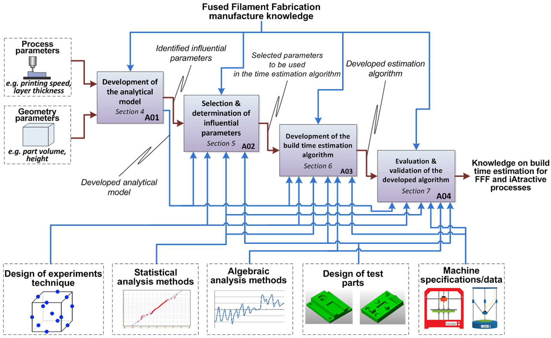
The method for developing the build time estimation algorithm.

Development of the analytical model

This section provides details on the development of the FFF analytical model. The parameters are divided into process and geometry parameters, which were then used in the analytical model development.

Process and geometry parameters

Build time (T_a) is defined as the amount of time that is required to fabricate a single or a group of parts in FFF. The estimation of build time involves a number of parameters to be taken into consideration. These parameters can be split into process parameters and geometry parameters:

Geometry parameters are the primary variables, and they have direct effect on build times no matter what AM process is used.

Process parameters are the controllable factors, and changing them can lead to the increase/decrease in build times. For example, increasing printing speed directly results in the reduction in build time.

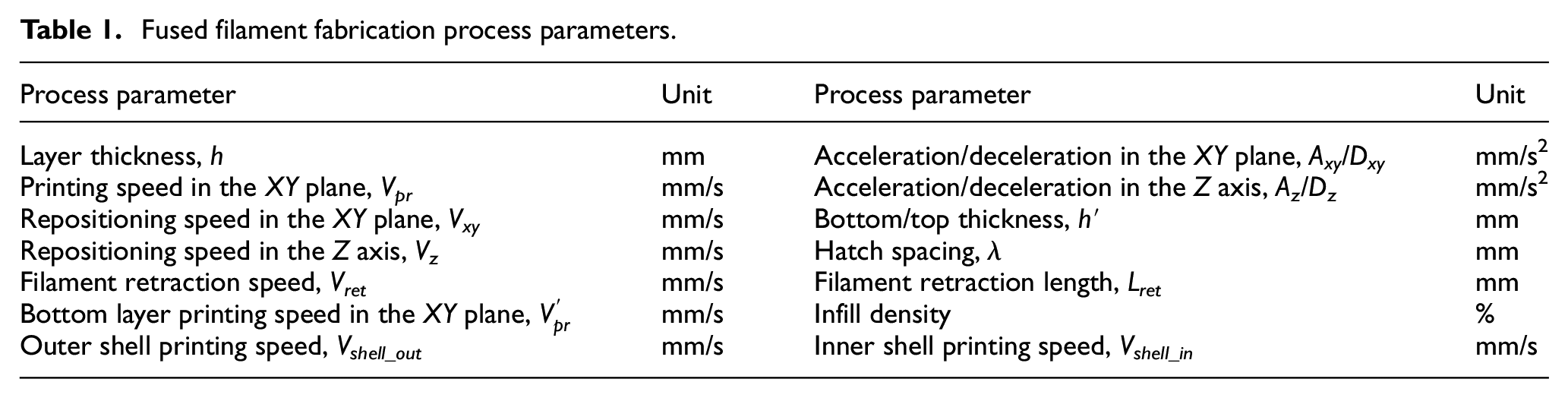
However, it has been reported that the change of process parameters affects the output quality of the printed parts, such as surface quality, dimensional accuracy and tensile strength.^22,41,42 The purpose of predicting build times is to identify the appropriate operation sequence which requires the least amount of build time. Despite the fact that changing the process parameters will most likely lead to the increase/decrease in build times, the aforementioned purpose cannot be achieved. This is because increasing or decreasing any or all of the speeds and accelerations/decelerations affects the entire FFF process, resulting in the increase or decrease in build times for producing the prototypes, respectively. Therefore, the process parameters were kept constant during the development of the estimation algorithm. The process parameters are summarised in Table 1, which will be used in the development of the analytical model in section ‘The FFF analytical model’.

Table 1.

Fused filament fabrication process parameters.

Process parameter	Unit	Process parameter	Unit
Layer thickness, h	mm	Acceleration/deceleration in the XY plane, A_xy/D_xy	mm/s²
Printing speed in the XY plane, V_pr	mm/s	Acceleration/deceleration in the Z axis, A_z/D_z	mm/s²
Repositioning speed in the XY plane, V_xy	mm/s	Bottom/top thickness, h′	mm
Repositioning speed in the Z axis, V_z	mm/s	Hatch spacing, λ	mm
Filament retraction speed, V_ret	mm/s	Filament retraction length, L_ret	mm
Bottom layer printing speed in the XY plane, $V_{pr}^{'}$	mm/s	Infill density	%
Outer shell printing speed, V_{shell_out}	mm/s	Inner shell printing speed, V_{shell_in}	mm/s

The FFF analytical model

Assuming that a part is sliced into N layers (N = |H/h|⁺ and | |⁺ represents the round up to the next integer number, H is the part height and h is the layer thickness), the overall build time of producing the part can be described as

T_{a} = \sum_{n = 1}^{N} T_{n} + T_{bed} + T_{heater} + T_{setup}

(1)

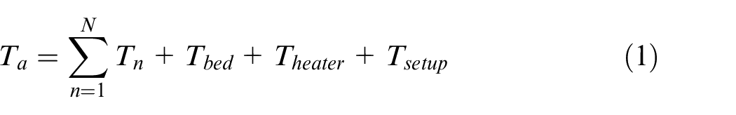
where T_bed is the time for warming up the bed to the material glass transition temperature (T_g) at which point the part stops warping; T_heater is the time used in turning on the heater for extruding material; T_n is the time used in printing the nth layer, n∈ [1, N]; and T_setup is the machine set-up time, which involves retreating and relocating of the deposition nozzle when switching from CNC machining to FFF. T_setup can be considered to be constant. Based on the practical printing experience, a uniform layer thickness (such as 0.2, 0.25 and 0.3 mm) can be used to print the entire part, that is, h′ = h. The FFF process is stable and the part quality is repeatable when using a uniform printing speed (e.g. $V_{pr} = V_{pr}^{'} = V_{shell_out} = V_{shell_in} = 60 mm / s$ ). For each layer, the build time T_n is divided into two parts, namely

T_{n} = T_{dep_n} + T_{idle_n}

(2)

where T_{dep_n} is the deposition time for the nth layer and T_{idle_n} is the idle time for the nth layer. Idle time includes deposition head repositioning time in the XY plane and Z axis (T_{rep_n_xy} and T_{rep_n_z}), which can be calculated using equation (3) below

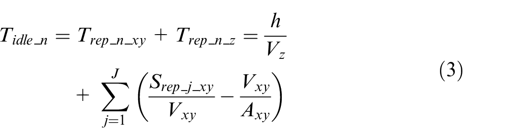
\begin{matrix} T_{idle_n} = T_{rep_n_xy} + T_{rep_n_z} = \frac{h}{V_{z}} \\ + \sum_{j = 1}^{J} (\frac{S_{rep_j_xy}}{V_{xy}} - \frac{V_{xy}}{A_{xy}}) \end{matrix}

(3)

where S_{rep_j_xy} is the jth (j∈ [1, J]) repositioning displacement (unit: mm) before depositing the jth continuous deposition path.

Deposition time (T_dep) is the time when the material is being extruded. Thus, the time used in depositing the nth layer is expressed in equation (4)

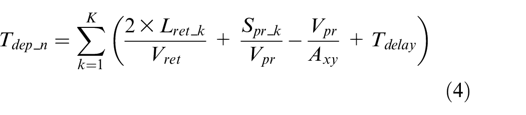
T_{dep_n} = \sum_{k = 1}^{K} (\frac{2 \times L_{ret_k}}{V_{ret}} + \frac{S_{pr_k}}{V_{pr}} - \frac{V_{pr}}{A_{xy}} + T_{delay})

(4)

where S_{pr_k} is the length of the kth (k∈ [1, K]) continuous deposition path; L_{ret_k} is the length of the filament retracted before depositing the kth deposition path; and T_delay is the delay time before depositing material on each individual continuous path.

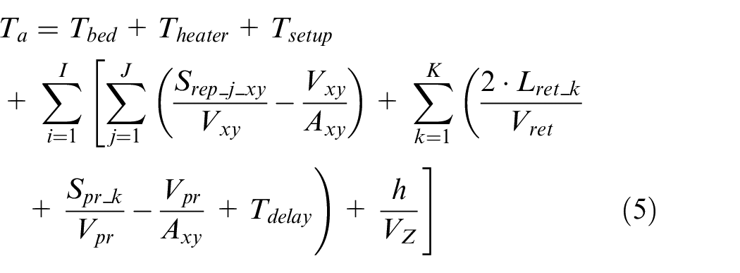
Based on the analysis outlined in the equations (1)–(5), a full representation of the build time for a single part is derived, as expressed below. It should be noted that this analytical model can only be used under the circumstances where the CAD model is sliced into a number of layers and the tool paths have been generated

T_{a} = T_{b e d} + T_{h e a t e r} + T_{s e t u p} + \sum_{i = 1}^{I} [\sum_{j = 1}^{J} (\frac{S_{rep_j_xy}}{V_{xy}} - \frac{V_{xy}}{A_{xy}}) + \sum_{k = 1}^{K} (\frac{2 \cdot L_{ret_k}}{V_{ret}} + \frac{S_{pr_k}}{V_{pr}} - \frac{V_{pr}}{A_{xy}} + T_{delay}) + \frac{h}{V_{Z}}]

(5)

Selection and determination of influential parameters

In this section, the process parameters to be investigated in the experiments are selected. This consists of initial selection of the parameters, determination of the parameters to be included in the estimation algorithm and the introduction of intermittent factor.

Initial selection of the parameters

Based on the analytical model above, the following statements are made:

Calculation of the build time using the analytical approach (equation (5)) is generally not practical at the operation sequencing stage¹³ in which only CAD models or 2D drawings are given.

Total length of deposition path (S_pr) primarily determines build times when certain printing speed and acceleration/deceleration are applied. Therefore, part volume (V) is considered as one of the major parameters that directly contributes to the total amount of build time.

Hatch spacing (λ) is represented in equation (5) by the use of S_pr. A high value of hatch spacing indicates low density of the part (i.e. the part is more porous), which in turn reduces the total length of the deposition path (S_pr). As a result, part density (ρ) is introduced in the build time estimation algorithm to represent λ and S_pr. Density is also defined as: density = 100% − part porosity.

Part height (H) has a direct effect on build time. Different heights of the part resulting from the change of part orientations can result in different build times.

Reducing the length of repositioning tool path (S_rep) could lead to decreases in machine idle time (T_idle). For each time the deposition head repositions, filament retraction and print delay (T_delay) are required, resulting in increased build time. The reasons that cause the head to reposition are (1) start printing next layer and (2) certain areas do not require material, such as printing pockets. Hence, the importance of head repositioning and the resulting idle time is investigated in section ‘Determination of the parameters’ in order to decide whether or not to include this parameter in the estimation algorithm.

Determination of the parameters

According to the statements made in section ‘Initial selection of the parameters’, test part A was designed (as shown in Figure 2) to evaluate the importance of deposition head repositioning time (i.e. idle time). The 2^k full factorial design of experiments (DoE) strategy was used. Five sets of parts with four different sizes of through pockets were designed. Producing rectangular blocks with pockets requires repositioning the deposition head repeatedly and frequently since the pockets do not need material. Every time the head travels across the pocket, it can be seen as a repositioning action. In order to avoid the effects caused by the varying volumes and heights, all parts in each set had the same volume and height but different pocket sizes as compared to the other parts in the same set. A density of 25% was also applied to all the parts.

Figure 2.

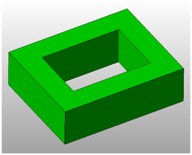
Test parts A.

The build times were calculated using the developed analytical model (equation (5)), which can be considered as the actual build times. The results (i.e. build times) were analysed using ANOVA, revealing that deposition head repositioning is a significant parameter in relation to total build times. The ANOVA results are shown in Table 2.

Table 2.

ANOVA table for length of repositioning tool path.

Source	Sum of squares	Degrees of freedom	Mean square	F-statistic	p value	F credit
Volume	44,986,349	4	11,246,587	517.53	<0.0001	3.26
Pocket	20,654,559	3	6,884,853	316.82	<0.0001	3.49
Error	260,773.2	12	21,731.1
Total	65,901,681	19

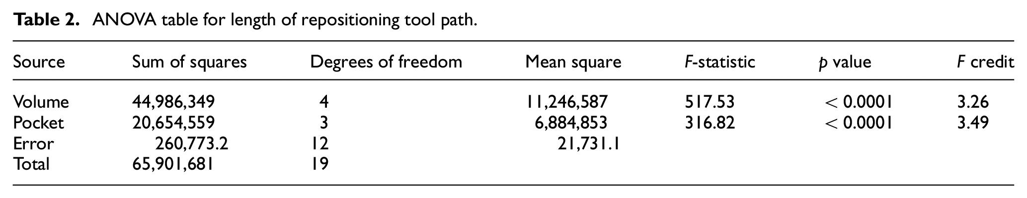
Due to F credit = 3.49 < F-statistic = 316.82, significant difference in build times has been identified while changing the length of repositioning tool path. The test demonstrates that build time is dependent not only on the total volume of the part but also on the distribution of material. Hence, length of repositioning tool path should be included in the build time estimation algorithm.

Intermittent factor

As stated in section ‘Introduction’, the parameters in the estimation algorithm should be obtainable from the CAD model and/or 2D drawings. However, from the test presented above, the distance travelled in repositioning and the number of times for repositioning cannot be obtained from the CAD model and/or drawings, which also depends on the part geometry and the slicing strategy employed. A term entitled intermittent factor (I) is therefore proposed to reflect the influence of the above two variables against total build time. A high intermittent factor implies that a significant amount of time is used in repositioning the deposition head and other relevant actions such as filament retraction and print delay. Assume that a feature (e.g. feature A) is sliced into a number of layers where discrete deposition areas exist. The intermittent factor can be calculated as the product of the ratio of discrete areas and STL boundary areas, and the ratio of feature A’s height and the height of outer feature that contains feature A.

To this end, part volume (V), part density (ρ), part height (H) and intermittent factor (I) were selected and defined to be investigated in the experiments for developing the estimation algorithm in sections ‘Developing the new build time estimation algorithm for FFF’ and ‘Evaluation and validation of the new build time estimation algorithm’. Among these four parameters, part volume and height can be directly obtained from the CAD model and/or drawings, part density is specified by the operator and the intermittent factor can be calculated based on the dimensions of the features.

Developing the new build time estimation algorithm for FFF

This section details the development of the new build time estimation algorithm consisting of test part design, design of experiments for the estimation algorithm development and experimental results, analysis and discussions.

Test part designs

There have already been several existing test parts for AM systems, but most of these parts were designed for accuracy evaluation only.⁴³ As introduced in section ‘Introduction’, the estimation algorithm will be used in process planning for the iAtractive process. Given that the iAtractive process is currently used to manufacture prismatic parts and the majority of engineering parts are prismatic or cylindrical in nature,³¹ the designs of the test parts (part B, C, D and E in Figure 3) include the full family of the prismatic features, namely, boss, pocket, slot, step, hole and planar face. Each of these test parts contains at least four different features and one combination of features, such as the combination of a step and a hole in test part B, and the combination of a boss and a pocket in test part C.

Figure 3.

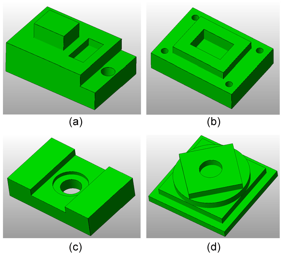
Test parts: (a) test part B, (b) test part C, (c) test part D and (d) test part E.

Design of experiments for the estimation algorithm development

Given that the four parameters are multi-level variables and their outcome effects are not linearly related, four levels were chosen to apply to part volume, height and density for each test part design. As the aim of the experiments was to develop the estimation algorithm rather than identify the influence of important factors only, the Taguchi method⁴⁴ was not considered to be appropriate. Another standard approach for DoE is to use the full factorial method. However, this method is only acceptable and feasible when a few (usually no more than three) factors are to be explored. For predicting build times, the more the experimental data obtained, the more accurate the prediction results. As a result, the levels of the parameters need to cover a wide range of values. For instance, it is better to investigate the influences caused by both small and large part volumes (small volume <50 cm³, medium volume 50–100 cm³ and large volume >100 cm³) and other volumes in between. Based on these reasons, the four test parts were increased in scale by a factor of 1.2, 1.4 and 1.6, by which the part volume and height vary accordingly. Four levels of part density, namely, 25%, 50%, 75% and 100% were used for each part volume and height variables. As a result, 64 experimental runs were required. The print settings are shown in Figure 4.

Figure 4.

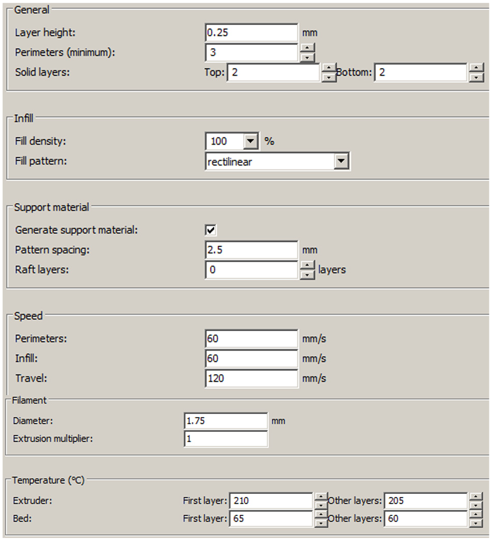
The FFF print settings.

Experimental results, analysis and discussions

To obtain the estimation algorithm, regression analysis and ANOVA were carried out iteratively. The errors were analysed by comparing the actual and the predicted build times to identify the importance of the interactions among the four control factors. By feeding back the error analysis, the final estimation algorithm was obtained, where unimportant interactions were removed. The actual build time (T_a) and the estimated build time $(T_{a}^{*})$ can be depicted in equations (6) and (7), respectively

\begin{matrix} T_{a} = f_{1} (V, H, ρ, I) + f_{2} (V, H, ρ, I) + \dots \\ + \sum_{p = 1}^{P} f_{i} (V, H, ρ, I) + T_{bed} + T_{heater} + T_{setup} \end{matrix}

(6)

\begin{matrix} T_{a}^{*} = C + f_{1}^{*} (V, H, ρ, I) + f_{2}^{*} (V, H, ρ, I) + \dots \\ + \sum_{q = 1}^{Q} f_{i}^{*} (V, H, ρ, I) + T_{bed} + T_{heater} + T_{setup} \end{matrix}

(7)

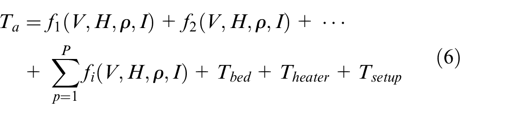
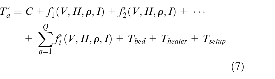
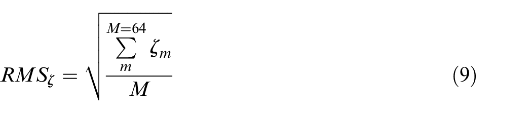
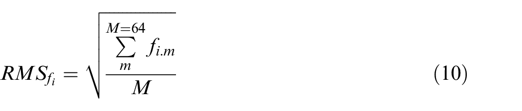
where f_i and $f_{i}^{*}$ are the functions related to part volume, height, density and intermittent factor in the analytical (actual) and the estimation algorithm, respectively. C is the intercept. Thus, the deviation (ζ_m) for each individual experiment can be expressed using equation (8)

ζ_{m} = | T_{total . m} - T_{total . m}^{*} |

(8)

where T_total.m is the actual build time in experiment m and $T_{total . m}^{*}$ is the estimated build time in experiment m. The root mean square of the deviation (RMS_ζ) and each function $(RM S_{f_{i}})$ in the estimation algorithm can be calculated using equations (9) and (10), where m denotes experiment number m

RM S_{ζ} = \sqrt{\frac{\sum_{m}^{M = 64} ζ_{m}}{M}}

(9)

RM S_{f_{i}} = \sqrt{\frac{\sum_{m}^{M = 64} f_{i . m}}{M}}

(10)

Given that producing a mid-range-sized prototype (i.e. 1.25 × 10² cm³) requires up to 7 h, the acceptable deviation between the actual and estimated build times was set to be 5 min. Therefore, for those $RM S_{f_{i}}$ that were one or more orders of magnitude greater than RMS_ζ, the corresponding functions were kept in the next run of the estimation algorithm development process. Other functions were removed from the algorithm. After five iterations, the final build time estimation algorithm was obtained as depicted in equation (11)

\begin{matrix} T_{a} = 168.33 + 23.56 V + 9.44 H + 160.19 V ρ \\ + 78.17 HI + T_{bed} + T_{heater} + T_{setup} + ε \end{matrix}

(11)

where ε is the uncertainty in the actual experiments.

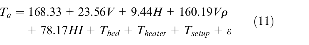
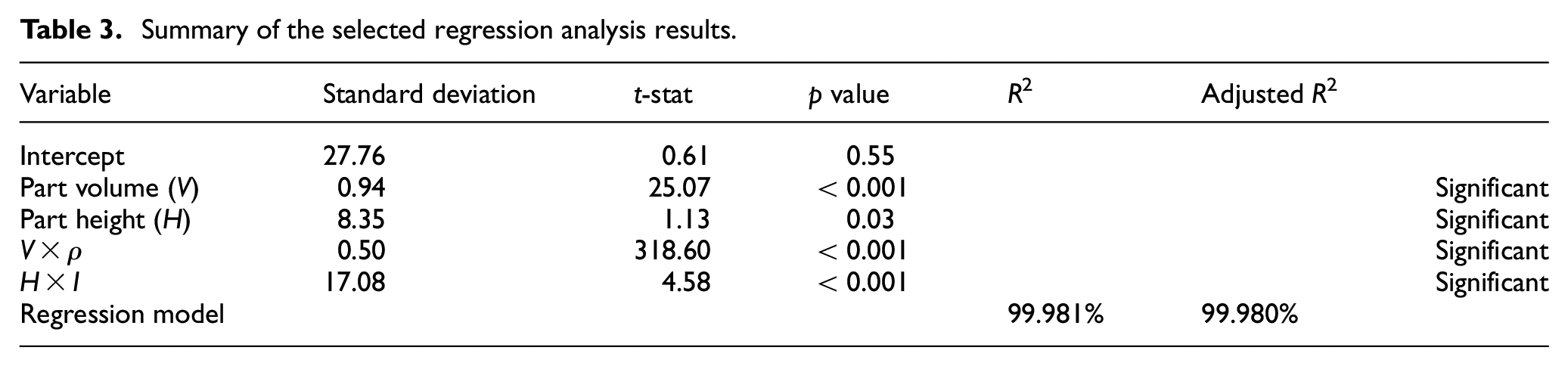
The selected analysis results are shown in Table 3, which were obtained by fitting the estimation algorithm as depicted in equation (11). Since the p values of part volume, the interaction of volume and density and the interaction of height and intermittent factor are significantly smaller than the threshold value of 5% in the analysis, they are of primary significance. Among them, the interaction of volume and density is the most significant factor, followed by part volume. With respect to the regression confidence (R²), the adjusted regression confidence ((R²)_adj) and the difference between them indicates that the regression model is satisfactory.

Table 3.

Summary of the selected regression analysis results.

Variable	Standard deviation	t-stat	p value	R ²	Adjusted R²
Intercept	27.76	0.61	0.55
Part volume (V)	0.94	25.07	<0.001			Significant
Part height (H)	8.35	1.13	0.03			Significant
V × ρ	0.50	318.60	<0.001			Significant
H × I	17.08	4.58	<0.001			Significant
Regression model				99.981%	99.980%

The residual analysis was carried out for checking the adequacy of the developed estimation algorithm. Figure 5 is the normal probability plot of the standardised residuals of the regression model (i.e. FFF build time estimation algorithm). It is considered as satisfactory due to the standardised residuals that are evenly distributed along the straight line. Figure 6 shows the distribution of the standardised residuals versus the experiment numbers. No distinct pattern has been observed, revealing that the current model is appropriate and no further factors are required for describing the relationship between the input factors and the estimated times. Approximately 98.4% of the standardised residuals fall in the interval (−2, +2), demonstrating that the errors are normally distributed. Nevertheless, it should also be noted that there are two points that are outside the interval. The standardised residual of one of the points is 2.01, which can still be considered as normal, but another standardised residual of 3.02 indicates the presence of an outlier. Thus, the parameters in the corresponding influential observation (experiment number 45) were traced back and the distance of the point from the average of all the points in the data set was recalculated. The results show that the outlier does not have a dramatic impact on the regression model. Figure 7 also supports this statement, which plots the errors curve showing that the error of 2.2% in experiment 45 is acceptable. Due to an unknown reason that caused the high-standardised residual, more tests were required to validate and evaluate the performance of the model, which will be presented in section ‘Evaluation and validation of the new build time estimation algorithm’.

Figure 5.

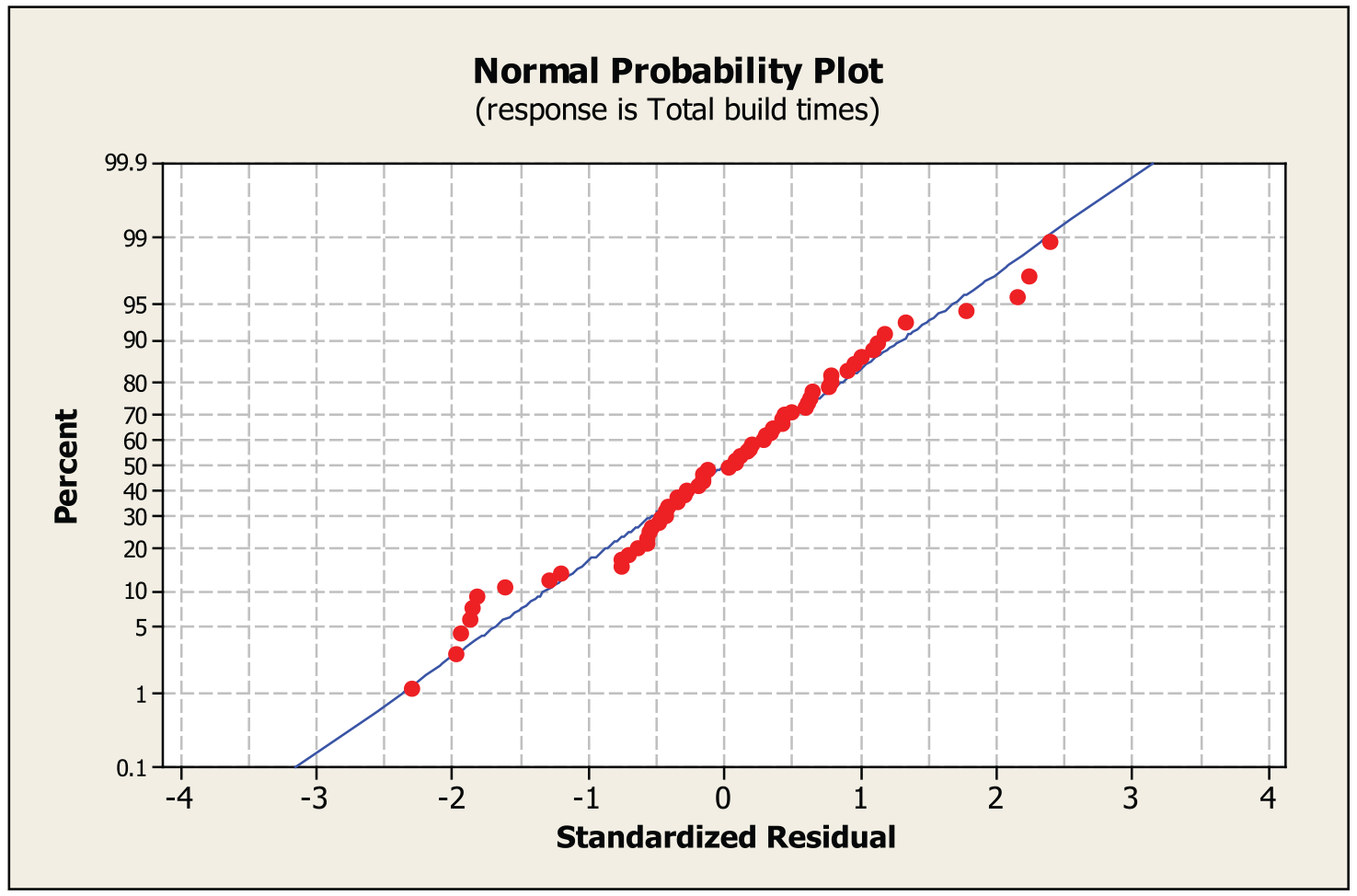
Normal probability plot of standardised residuals.

Figure 6.

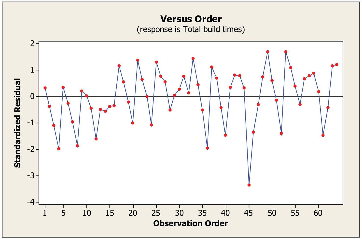
Distribution of standardised residuals versus experiment number.

Figure 7.

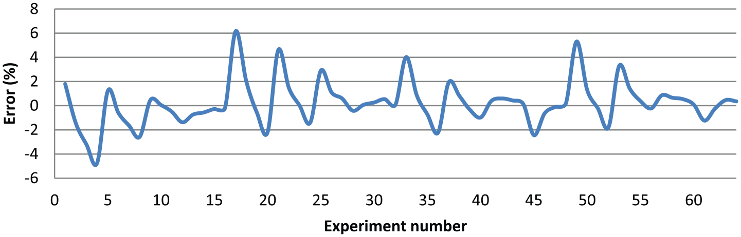
Percentage error between the actual and estimated build times for the test parts in the estimation algorithm development.

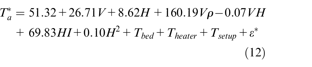
It is noted that the errors tend to increase while the part volume is small, as identified in Figure 7. While the four test parts were not scaled up (experiment 1–4, 17–20, 33–36 and 49–52), the errors are relatively larger than the errors in other experiments. In addition, the original volumes of test parts D and F are small (less than 50 cm³). As a result, the errors do not decrease significantly while the parts were scaled up 1.2 times. An exact reason cannot be provided, however, for small and medium parts where the volume does not exceed 100 cm³, even though the number of repositioning and filament retraction times are kept unchanged, the length of the repositioning tool path is significantly shorter than that of the larger volume parts, while the intermittent factors are identical. This may lead to an increase in estimation error. Furthermore, it is worth mentioning that errors can be simply reduced to lower than 1% by expanding equation (11) with additional factors (e.g. adding interactions between V, H, ρ and I, as shown in equation (12) as an example)

\begin{matrix} T_{a}^{*} = 51.32 + 26.71 V + 8.62 H + 160.19 V ρ - 0.07 VH \\ + 69.83 HI + 0.10 H^{2} + T_{bed} + T_{heater} + T_{setup} + ε^{*} \end{matrix}

(12)

Evaluation and validation of the new build time estimation algorithm

Upon obtaining positive results from the previous experiments, two case studies were conducted for the evaluation and validation of the build time estimation algorithm and are detailed below.

Case study I

Design of experiments for case study I

The test parts designed in this section include various features, as shown in Figure 8, and more importantly, fabricating these features requires varying length of repositioning tool paths and differing number of repositioning and filament retraction times. Test parts F and H were modified based on the parts designed by Kechagias et al.³⁰ and Zhou et al.,⁴⁵ respectively. Test part H contains nine features including planar face, boss, pocket, sphere and chamfer.

Figure 8.

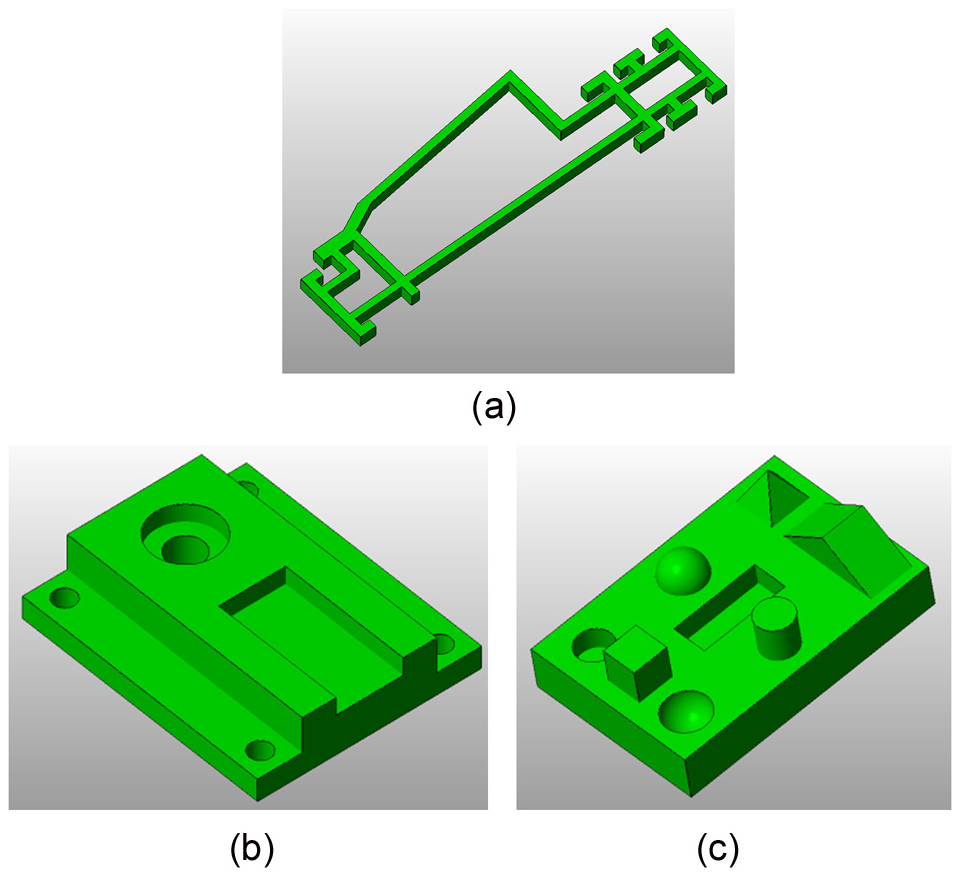
Test parts: (a) test part F, (b) test part G and (c) test part H.

It was found that the majority of the estimation inaccuracy lies in producing parts with a volume of less than 50 cm³. Therefore, the volumes of test parts G and H were specifically designed to be less than 50 cm³. Subsequently, the three original test parts were scaled up 1.2, 1.4 and 1.6 times, generating 12 test parts with differing part volumes and heights. Due to the interaction of volume and porosity that is the most significant factor, 25%, 50%, 75% and 100% levels of porosity were applied to these 12 test parts. As a result, a total of 48 test parts were defined.

Experimental results and analysis for case study I

Table 4 presents the results obtained in the experimental runs 17–32. The errors between the estimated and the actual build times are also presented. It is observed that the errors for the part volume of 45 cm³ could be up to −6.73%, whereas the largest error is only 0.75% for the part volume of 187.11 cm³. With the increase in part volume, the mean error gradually reduces from 3.44% to 0.36%.

Table 4.

The predicted build times using the developed estimation algorithm.

Experimentnumber	Volume (cm³)	Height (mm)	Porosity (%)	Intermittentfactor	Actual buildtime (s)	Estimated buildtime (s)	Error (%)
17	45.68	20	25	0.14	3735	3484	−6.73
18	45.68	20	50	0.14	5365	5313	−0.97
19	45.68	20	75	0.14	7012	7142	1.86
20	45.68	20	100	0.14	8609	8972	4.21
21	78.94	24	25	0.14	5981	5681	−5.02
22	78.94	24	50	0.14	8962	8842	−1.34
23	78.94	24	75	0.14	11,931	12,003	0.60
24	78.94	24	100	0.14	14,794	15,164	2.50
25	125.35	28	25	0.14	8982	8715	−2.98
26	125.35	28	50	0.14	13,866	13,734	−0.95
27	125.35	28	75	0.14	18,670	18,754	0.45
28	125.35	28	100	0.14	23,493	23,774	1.19
29	187.11	32	25	0.14	12,788	12,725	−0.50
30	187.11	32	50	0.14	20,220	20,218	−0.01
31	187.11	32	75	0.14	27,661	27,711	0.18
32	187.11	32	100	0.14	34,941	35,204	0.75

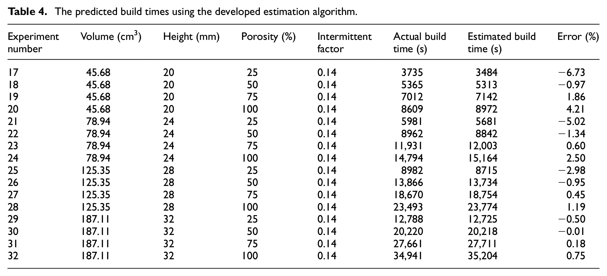
The percentage errors between the predicted and actual times are plotted in Figure 9. The average error is 6.7%; the best results were obtained in the experimental runs 17–32, and there is no obvious fluctuation (less than 13.5% error) in the experimental runs 1–16 and 33–48. As the estimation algorithm (equation (11)) only has four factors rather than six (equation (12)), it is not as sensitive as equation (12) in terms of prediction accuracy when a large number of repositioning movements are required for building a part. The test parts in the experiments 17–32 (test part G and variations) have a low intermittent factor (less than 0.2), indicating the short length of repositioning tool paths, relatively low number of repositioning and filament retraction times, as well as a short resulting delay time during production. Thus, the resulting errors were reduced. In other words, the developed estimation algorithm has better performance for parts with a low intermittent factor (<0.2). The predicted times tend to be longer than the actual times while the algorithm is applied to parts with a high intermittent factor (>0.5).

Figure 9.

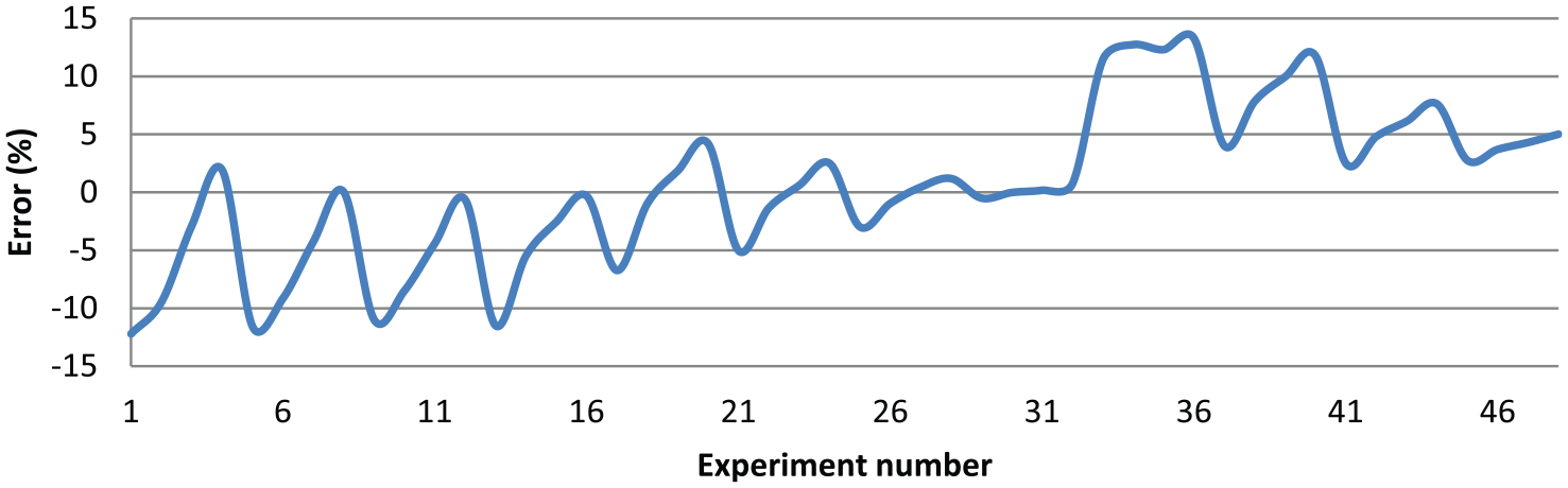
Percentage error between the actual and estimated build times for the test parts in the estimation algorithm evaluation.

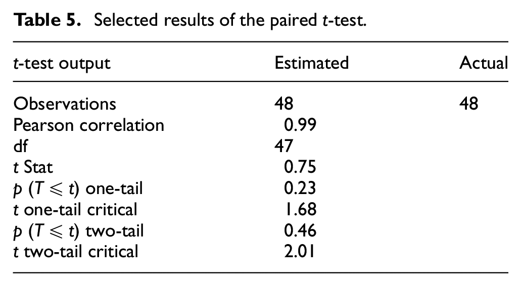
In order to evaluate the algorithm, a statistical method, namely, t-tests was used to analyse the results, identifying whether significant difference exists between the estimated and actual build times. Paired t-tests were carried out for all the test parts at a 95% confidence interval for the analysis of the differences between the estimated and actual times. The selected results are listed in Table 5, where t-stat is 0.75 < t two-tail critical = 2.01 (α = 0.05). Thus, it can be concluded that the build time estimation algorithm does not yield significantly different results when compared with the actual times.

Table 5.

Selected results of the paired t-test.

t-test output	Estimated	Actual
Observations	48	48
Pearson correlation	0.99
df	47
t Stat	0.75
p (T ≤ t) one-tail	0.23
t one-tail critical	1.68
p (T ≤ t) two-tail	0.46
t two-tail critical	2.01

Case study II

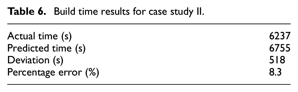
An engineering part shown in Figure 10 was used to further test the validity of the developed estimation algorithm. The volume and height of the part are 26.67 × 10³ mm³ and 31 mm, respectively. As it is an engineering part, the part density is specified as 100% solid. Based on the dimensions, the intermittent factor can be calculated, which is 0.575. The estimated results are listed in Table 6, and the percentage error is 8.3%, demonstrating the efficacy of this new proposed algorithm.

Figure 10.

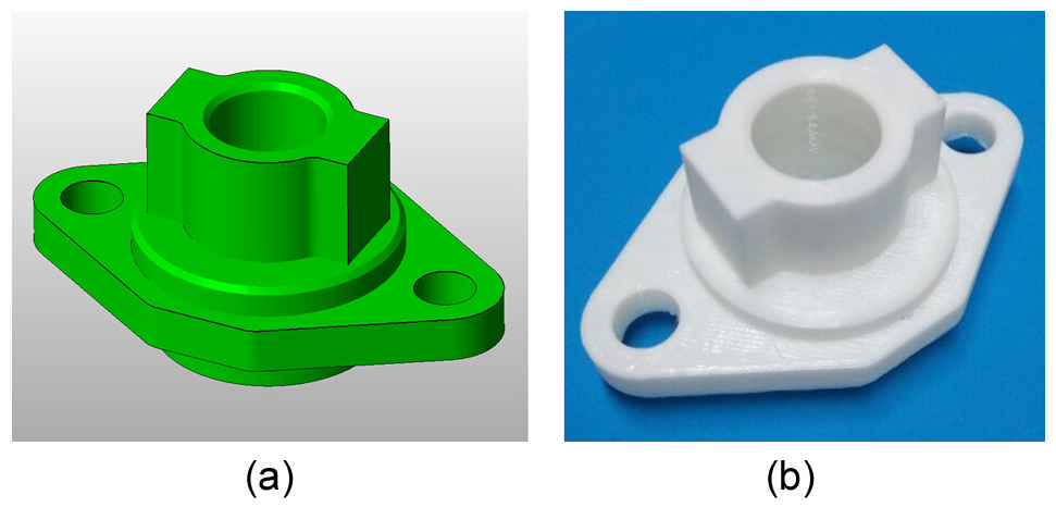
An engineering part for case study II: (a) CAD model and (b) the printed part.

Table 6.

Build time results for case study II.

Actual time (s)	6237
Predicted time (s)	6755
Deviation (s)	518
Percentage error (%)	8.3

Discussion on the new build time estimation algorithm

Based on the case studies and analysis, it can be identified that the developed estimation algorithm is able to predict build times and the predicted results do not have significant difference to the actual times. In comparison to other estimators,^{28,30,31,35,38} this estimation algorithm offers a time-saving method, which only requires the part dimensions, that is, 2D drawings. This eliminates considerable time used in slicing CAD models and post-processing them for build time calculation.

While the advantages of the proposed method have been documented and described, there are a number of other issues that need to be addressed. First, the algorithm shows advantages only for parts in which all the features involved are prismatic. However, it is currently not suitable for parts with sculptured free-form surfaces because the intermittent factor cannot precisely represent properties of such structures. Although it is possible to approximate shapes and volumes contained by free-form surfaces into a large number of prisms, Campbell et al.³¹ pointed out that estimated build times might still remain inaccurate. The major advantage of this algorithm is high efficiency, which is able to estimate build times based on the part dimensions in 2D drawings. As such, the algorithm only includes the four most significant factors documented in section ‘Selection and determination of influential parameters’. In the future, efforts will be made to enhance the functionality and accuracy of the algorithm for precisely predicting times for sculptured surfaces. A possible solution is to employ a correction factor used by Pham and Wang,²⁴ which partly depends on the ratio of the part volume to the volume of a bounding box around the STL file. By introducing this factor, more attributes including geometry complexity, wall thickness and the number of parts to be fabricated in one single set-up can be taken into consideration.

Furthermore, the estimation algorithm is developed based on the deposition of polylactic acid (PLA) and the layer thickness of 0.25 mm. PLA is now one of the most widely used materials for FFF. Changing material such as acrylonitrile butadiene styrene (ABS) will affect build time and the firmware of the FFF system will automatically adjust the relevant speeds accordingly, such as printing and travelling speeds of the deposition head, to ensure correct printing. Printing ABS is more time intensive when compared to PLA because the deposition head needs to go slower to allow for heat dissipation, requiring more time to cool the part to prevent overheating and lose of printing details. The printing temperatures for PLA and ABS are 200 °C and 240 °C–260 °C, respectively. The main difference between printing PLA and ABS is welding. PLA creates an extremely strong weld to itself so that cooling fans can be used to accelerate the cooling process. In contrast, ABS bonds to itself very weakly, therefore adding cooling fans makes this worse and can initiate cracking. The relatively slow printing of ABS is also due to its T_g being higher than PLA. Although the method proposed in section ‘The method for developing a new build time estimation algorithm for FFF’ can still be used to develop a new estimation algorithm when material, layer thickness and other parameters are changed, it would still be better to introduce an adjustment factor into the current developed algorithm, which is able to adjust estimated results based on different materials and layer thicknesses. Additionally, equation (5) in section ‘The FFF analytical model’ can always be used to accurately calculate build times for different materials in the circumstances where the CAD model is sliced into layers and the tool paths are generated.

For different types of system, namely Cartesian and Delta systems, the key difference between them lies in the motion control mechanism, which can affect the dimensional accuracies of the printed parts. For low printing speeds (i.e. <80 mm/s), both Cartesian and Delta systems are able to fabricate parts, achieving the same (or very close) dimensional accuracies. However, for high printing speeds (i.e. >80 mm/s), the Delta system usually shows better dimensional accuracy due to the low rotatory inertia of the motors for motion control and the low accumulative error in the XY plane. With respect to the build time for printing a part, the printing speed is defined by a user and then coded in a programme called G-Code, which is similar to numerical control (NC) codes for CNC machines. Thus, as long as the same G-Code is used, the build times will be the same no matter which system the part is printed by. In this study, the printing speed of 60 mm/s is used, which is the most stable and widely used speed for Cartesian FDM machines, such as Stratasys FDM.⁴⁰ Further to the filament diameter, it barely affects actual build times. This is because, for printing the same object, the build time is dependent on printing and travelling speeds of the deposition head. Based on the given speeds, the firmware calculates feed rate of the filament that is fed into the liquefier chamber. The feed rates for filament of φ1.75 or 3 mm may be different; however, the volumes of the semi-melted material extruded from the nozzle per unit time are the same.

Limitations and constraints in the development of the estimation algorithm

This subsection summarises the limitations of the estimation algorithm and the constraints that led to the limitations during the algorithm development process:

Relatively simple features. The estimation algorithm has been developed to predict FFF build times for prismatic parts in the context of hybrid manufacture. While the iAtractive process¹³ is currently aimed at producing difficult-to-cut (internal structures) prismatic parts, the future trend is to realise high precision manufacture of both internal features and sculptured free-form surfaces.

Few factors considered. Only four factors, that is, volume, height, density and intermittent factor, are taken into consideration due to the efficiency consideration in process planning for the iAtractive process. Process planning requires fast and efficient time estimation based on 2D drawings (feature dimensions), which are the most accessible geometrical information for the iAtractive process. This requirement has imposed a constraint to the estimation algorithm. Adopting existing time estimation methods presented in the papers^{26–30,35,38} is not viable since these methods need to further process the given CAD model (i.e. slicing it into layers and generating tool paths for the deposition head). Due to the limited number of factors included in the authors’ estimation algorithm, it is currently not able to provide high estimation accuracy for sculptured free-form surfaces. An effective approach to improving the accuracy, as identified in equation (12), is to increase the number of factors in the algorithm.

Limited choices of FFF process parameters. The estimation algorithm was investigated in the condition where the material, layer thickness, printing speeds and infill patterns were set as PLA, 0.25 mm, 60 mm/s and rectilinear, respectively, which are the FFF recommended settings.⁴⁶ This limitation has constrained a user from defining his or her preferred printing parameters and values for customised products.

Diminished estimation accuracy in predicting times for printing an array of parts (multiple objects). Parts are sometimes preferred to be fabricated simultaneously in a single FFF operation, in which case a large number of parts are arranged on a build platform with certain distances (defined by the user) with each other. This leads to an increase in the repositioning displacement (S_{rep_j_xy}) (see equation (5)), which further results in the increased proportion of time in repositioning the deposition head from one-part cross-section to another. The predicted build time is likely to be less accurate due to the poor predictions of the repositioning time.

Conclusion and future work

In this article, a new build time estimation algorithm for the FFF process under the context of hybrid manufacturing has been developed. The input for the algorithm can be directly obtained from the part dimensions/drawings, providing a new, accurate and efficient approach to time estimation. The method for developing the algorithm was described and consisted of four major stages as described in Figure 1. The analytical model was first created to analyse process and geometry parameters. This analytical model was then used in the later stages to accurately calculate build times. The selection of influential parameters, the estimation algorithm development and evaluation were carried out in sequence. A robust experimental approach was used consisting of a design of experiments approach, and the results were statistically analysed and discussed at each stage. Part volume, height, porosity and intermittent factor together with their interactions have been identified as the significant parameters that affect build times. The estimation algorithm is capable of predicting build times with an average error of 6.7%, the maximum error of 13.5% on the total build time and 80% of this error falls within an 8% deviation. The statistical analysis indicates that no significant difference was found between the estimated and actual build times. In addition, deviation is likely to increase for parts with a large intermittent factor (>0.5) or volume of less than 50 cm³. This clearly demonstrates the significance of this work and its influence on the emerging domain of hybrid manufacture. The build time estimation algorithm differs from existing methods by being able to directly predict build times based on part dimensions without the need to further process the CAD model or run complex algorithms. This provides a more fluid and robust method to predict build times. Beneficiaries of this new algorithm will be manufacturing engineers who fabricate functional parts using AM or hybrid processes and designers who build prototypes to evaluate and validate designs.

Future work will focus on implementation of this new algorithm for build time estimation on a wide range of AM methods particularly aligned to the combination of additive and subtractive manufacturing technologies. Further enhancements to the functionality of the algorithm to provide accurate prediction of build times for free-form complex surfaces and components will be made. This may require an extra parameter to compensate for the intermittent factor to reflect geometry complexity and changes in part volume.

Footnotes

Declaration of Conflicting Interests

The author(s) declared no potential conflicts of interest with respect to the research, authorship and/or publication of this article.

Funding

The author(s) received no financial support for the research, authorship and/or publication of this article.

References

Lauwers

Klocke

Klink

. Hybrid processes in manufacturing. CIRP Ann: Manuf Techn 2014; 63: 561–583.

Fonda

Nakamoto

Heidari

. A study on the optimal fabrication method for micro-scale gyroscopes using a hybrid process consisting of electric discharge machining, chemical etching or micro-mechanical milling. CIRP Ann: Manuf Techn 2013; 62: 183–186.

Zhang

Wang

. Hybrid direct manufacturing method of metallic parts using deposition and micro continuous rolling. Rapid Prototyping J 2013; 19: 387–394.

Karunakaran

Bernard

Suryakumar

. Rapid manufacturing of metallic objects. Rapid Prototyping J 2012; 18: 264–280.

Newman

Zhu

Dhokia

. Process planning for additive and subtractive manufacturing technologies. CIRP Ann: Manuf Techn 2015; 64: 467–470.

Zhu

Dhokia

Nassehi

. A review of hybrid manufacturing processes – state of the art and future perspectives. Int J Comput Integ M 2013; 26: 596–615.

Simhambhatla

Karunakaran

Build strategies for rapid manufacturing of components of varying complexity. Rapid Prototyping J 2015; 21: 340–350.

Karunakaran

Suryakumar

Pushpa

. Low cost integration of additive and subtractive processes for hybrid layered manufacturing. Robot CIM: Int Manuf 2010; 26: 490–499.

Nagel

JKS

Liou

. Hybrid manufacturing system modeling and development. In: ASME 2012 international design engineering technical conferences and computers and information in engineering conference, Chicago, IL, 12–15 August 2012, pp.189–198. New York: American Society of Mechanical Engineers (ASME).

10.

Ren

Sparks

Ruan

. Integrated process planning for a multiaxis hybrid manufacturing system. J Manuf Sci E: T ASME 2010; 132.

11.

Lee

Wei

Chung

. Development of a hybrid rapid prototyping system using low-cost fused deposition modeling and five-axis machining. J Mater Process Tech 2014; 214: 2366–2374.

12.

Xiong

Haiou

Guilan

. Hybrid plasma deposition and milling for an aeroengine double helix integral impeller made of superalloy. Robot CIM: Int Manuf 2009; 26: 291–295.

13.

Zhu

Dhokia

Newman

. Application of a hybrid process for high precision manufacture of difficult to machine prismatic parts. Int J Adv Manuf Tech 2014; 74: 1115–1132.

14.

Zhu

Dhokia

Newman

. A novel decision-making logic for hybrid manufacture of prismatic components based on existing parts. J Intell Manuf. Epub ahead of print 24 September 2014. DOI: 10.1007/s10845-014-0966-8.

15.

Zhu

Dhokia

Newman

. The development of a novel process planning algorithm for an unconstrained hybrid manufacturing process. J Manuf Process 2013; 15: 404–413.

16.

Jones

Haufe

Sells

. RepRap – the replicating rapid prototyper. Robotica 2011; 29: 177–191.

17.

Wang

Chen

. An integrated optimization of cutting parameters and tool path generation in ultraprecision raster milling. Int J Adv Manuf Tech 2014; 75: 1711–1721.

18.

Heo

Kim

. Estimation of NC machining time using NC block distribution for sculptured surface machining. Robot CIM: Int Manuf 2006; 22: 437–446.

19.

Jung

Park

. Five-axis machining time estimation algorithm based on machine characteristics. J Mater Process Tech 2007; 187: 37–40.

20.

Jin

Gao

. An adaptive process planning approach of rapid prototyping and manufacturing. Robot CIM: Int Manuf 2013; 29: 23–38.

21.

Han

Fafari

Seyed

. Process speeding up via deposition planning in fused deposition-based layered manufacturing processes. Rapid Prototyping J 2003; 9: 212–218.

22.

Turner

Gold

. A review of melt extrusion additive manufacturing processes: II. Materials, dimensional accuracy, and surface roughness. Rapid Prototyping J 2015; 21: 250–261.

23.

Jin

Gao

. A hybrid and adaptive tool-path generation approach of rapid prototyping and manufacturing for biomedical models. Comput Ind 2013; 64: 336–349.

24.

Pham

Wang

. Prediction and reduction of build times for the selective laser sintering process. Proc IMechE, Part B: J Engineering Manufacture 2000; 214: 425–430.

25.

Teitelbaum

Schmidt

Goaer

. Examining potential design guidelines for use in fused deposition modeling to reduce build time and material volume. In: ASME 2009 international design engineering technical conferences and computers and information in engineering conference, San Diego, CA, 30 August–2 September 2009, pp.73–82. New York: American Society of Mechanical Engineers (ASME).

26.

Yim

Rosen

. Build time and cost models for additive manufacturing process selection. In: ASME 2012 international design engineering technical conferences and computers and information in engineering conference, Chicago, IL, 12–15 August 2012, pp.375–382. New York: American Society of Mechanical Engineers (ASME).

27.

Huang

Singamneni

. Adaptive slicing and speed- and time-dependent consolidation mechanisms in fused deposition modeling. Proc IMechE, Part B: J Engineering Manufacture 2014; 228: 111–126.

28.

Nezhad

Vatani

Barazandeh

. Build time estimator for determining optimal part orientation. Proc IMechE, Part B: J Engineering Manufacture 2010; 224: 1905–1913.

29.

Ghorpade

Karunakaran

Tiwari

. Selection of optimal part orientation in fused deposition modelling using swarm intelligence. Proc IMechE, Part B: J Engineering Manufacture 2007; 221: 1209–1220.

30.

Kechagias

Maropoulos

Karagiannis

. Process build-time estimator algorithm for laminated object manufacturing. Rapid Prototyping J 2004; 10: 297–304.

31.

Campbell

Combrinck

de Beer

. Stereolithography build time estimation based on volumetric calculations. Rapid Prototyping J 2008; 14: 271–279.

32.

Ruffo

Tuck

Hague

. Empirical laser sintering time estimator for Duraform PA. Int J Prod Res 2006; 44: 5131–5146.

33.

Ruffo

Tuck

Hague

. Cost estimation for rapid manufacturing-laser sintering production for low to medium volumes. Proc IMechE, Part B: J Engineering Manufacture 2006; 220: 1417–1427.

34.

Kumar

Regalla

. Optimization of support material and build time in Fused Deposition Modeling (FDM). In: Fan

(ed.) Mechanical and aerospace engineering, parts 1–7. Zurich: Trans Tech Publications Ltd, 2012, pp.2245–2251.

35.

Baumers

Tuck

Wildman

. Transparency built-in energy consumption and cost estimation for additive manufacturing. J Ind Ecol 2013; 17: 418–431.

36.

Baumers

Dickens

Tuck

. The cost of additive manufacturing: machine productivity, economies of scale and technology-push. Technol Forecast Soc 2016; 102: 193–201.

37.

Munguía

Ciurana

Riba

. Neural-network-based model for build-time estimation in selective laser sintering. Proc IMechE, Part B: J Engineering Manufacture 2009; 223: 995–1003.

38.

Di Angelo

Di Stefano

. A neural network-based build time estimator for layer manufactured objects. Int J Adv Manuf Tech 2011; 57: 215–224.

39.

Ultimaker . Ultimaker Cura Software – you and cura made for each other. 2015, http://www.Ultimaker.com

40.

Stratasys . CatalystEX software for dimension elite. 2015, http://www.stratasys.com

41.

Durgun

Ertan

. Experimental investigation of FDM process for improvement of mechanical properties and production cost. Rapid Prototyping J 2014; 20: 228–235.

42.

Boschetto

Bottini

. Accuracy prediction in fused deposition modeling. Int J Adv Manuf Tech 2014; 73: 913–928.

43.

Brajlih

Valentan

Balic

. Speed and accuracy evaluation of additive manufacturing machines. Rapid Prototyping J 2011; 17: 64–75.

44.

Ross

. Taguchi techniques for quality engineering: loss function, orthogonal experiments, parameter and tolerance design. New York: McGraw-Hill Professional, 1996.

45.

Zhou

Herscovici

Chen

. Parametric process optimization to improve the accuracy of rapid prototyped stereolithography parts. Int J Mach Tool Manu 2000; 40: 363–379.

46.

Bowyer

. Driver software – RepRap Host Software. 2015, http://reprap.org/wiki/Reprap_host_software

A new algorithm for build time estimation for fused filament fabrication technologies

Abstract

Keywords

Introduction

Review of build time estimation research

The method for developing a new build time estimation algorithm for FFF

Development of the analytical model

Process and geometry parameters

The FFF analytical model

Selection and determination of influential parameters

Initial selection of the parameters

Determination of the parameters

Intermittent factor

Developing the new build time estimation algorithm for FFF

Test part designs

Design of experiments for the estimation algorithm development

Experimental results, analysis and discussions

Evaluation and validation of the new build time estimation algorithm

Case study I

Design of experiments for case study I

Experimental results and analysis for case study I

Case study II

Discussion on the new build time estimation algorithm

Limitations and constraints in the development of the estimation algorithm

Conclusion and future work

Footnotes

Declaration of Conflicting Interests

Funding

References