Variable dimensional chain of stroke-related mechanical assemblies

Abstract

In traditional assembly dimensional chain theory, actual geometrical features are obtained by translating or rotating from the nominal geometrical features. Thus, the deviation stack-up function is irrelevant with the machining stroke. In order to solve this problem, a model describing the variation in the dimensional chain of stroke-related mechanical assemblies is proposed. The geometrical features of assembly parts are discretized as a set of coordinate points, and the traditional geometrical dimensional chain is equivalently replaced by several linear dimensional chains. For every linear dimensional chain, the assembly datum of two parts is deformed due to gravity or thermal effect and so on, resulting in the non-closure of dimensional chain. In this article, the closure of the dimensional chain is guaranteed by replacing the assembly datum by the plane determined by three highest points. Finally, an experiment was carried out to verify the necessity of constructing the variable dimensional chain and its accuracy. Combining this new model with Monte Carlo simulation method, the influence of gravity on tolerance analysis was analyzed, and the results show that the variation in the dimensional chain induced by working conditions cannot be ignored in the tolerance design stage.

Introduction

Tolerance analysis is used to determine the accumulative effect between the tolerances of functional elements (FEs) and functional requirement (FR). A typical tolerance analysis process consists of three major steps. The first step is tolerance modeling where mathematical model is derived to describe the dimensional or geometrical variations in the parts. The second step is establishing the deviation stack-up function of mechanical assemblies, which describes the accumulative effects between the dimensional or geometrical deviations of FEs and FR. In the last step, the accumulative effect between the tolerances of FEs and FR is acquired by combining the established deviation stack-up function with the worst-case, root sum square or Monte Carlo simulation methods.

Currently, the major tolerance models include attribute models, ¹ offset zone models, ² parametric models, ³ kinematic models ⁴ and degree of freedom models. ⁵ In International Organization for Standardization (ISO) standard ⁶ and these models, actual geometrical features are obtained by translating or rotating from the nominal geometrical features. Consequently, the variation in the deviation stack-up function of stroke-related mechanical assemblies cannot be described. Based on the tolerance models, tolerance analysis is used to determine whether the designed tolerances of FEs could satisfy the tolerance requirement of FR.

Constructing the deviation stack-up function of mechanical assemblies is the most important step of tolerance analysis. Tolerance analysis models include tolerance analysis models based on homogeneous transformation matrix (HTM), Jacobian models, vector-loop based model and Tolerance-Map^®. The tolerance analysis model based on HTM was proposed by Whitney et al. ⁷ Desrochers and Clément, ⁸ Desrochers ⁹ and Guo et al. ¹⁰ used this approach. In this model, geometrical features are discretized as coordinate points, and the actual geometrical features are replaced by the fitting surface or line of the discretized points. Accordingly, the HTM between two mechanical assemblies is derived. This model is mainly used in deviation evaluation of FR when the orientation deviation of FE is much larger than its form deviation. However, the prediction accuracy of this model is poor while the form deviation of FE is much bigger than its orientation deviation. Jacobian models proposed by Laperrière and colleagues,^11,12 Ghie et al. ¹³ and Desrochers et al. ¹⁴ take HTM as its foundation. The Jacobian matrix between two mechanical assemblies is obtained to describe the deviation stack-up function of mechanical assemblies, and the tolerance accumulative effects between FEs and FR are acquired by combining this model with modal interval arithmetic and so on. Because of the construction of HTM in this model, the weakness of this model is the same as the model based on HTM. The vector-loop-based model was proposed by Chase ¹⁵ and Gao et al. ¹⁶ This model uses vectors to represent dimensions in an assembly and create the assembly graph. This model also relies on the construction of HTM. The tolerance-mapping (T-Map) was first proposed by Davidson et al. ¹⁷ Both Mujezinovic et al. ¹⁸ and Singh et al. ¹⁹ used this model. In this model, the variation in geometrical features in tolerance zone is “reflected” by the volume of the assumed point set. T-Map must combine with Minkowski sum to accomplish the tolerance analysis process.

The variation in the deviation stack-up function cannot be described in these models. However, this variation in the deviation stack-up function is often large for stroke-related mechanical assemblies. The horizontal machining center was taken as an example in this paper. According to ISO 10791-1: 1998, ²⁰ there are four form tolerance requirements and 22 position tolerance requirements, but no size tolerance requirements. Except for flatness, axial runout and radial runout, there are 23 tolerance requirements associated with the machining stroke. Especially, for the large machine tool components, such as the bed, the column and the beam, the variation in dimensional or geometrical deviations in the whole machining stroke is very large due to some affecting factors such as gravity of the moving components. In this article, a verification experiment was carried out on a horizontal machining center, as shown in Figure 6. The calculation results in section “Necessity of constructing the variable dimensional chain” show that the variation in FR is 6.1 µm in the whole machining stroke due to the gravity of the moving components, while the FR of the straightness of the X-axis motion is 6 µm. So the variation in FR cannot be ignored. However, the variation in the deviation stack-up function of mechanical assemblies cannot be derived from the models based on HTM and so on.

Hence, this article presents a variable dimensional chain in which the variation in the deviation stack-up function could be considered. First, the coordinate systems of the mechanical assemblies are set according to the actual testing requirements. In order to describe the variation in the geometrical features under working conditions, the geometrical features of assembly parts are discretized as a set of coordinate points in this model. Then a mathematical model of geometrical tolerance is constructed by limiting the coordinates of the points in the form of inequalities. Second, the traditional geometrical dimensional chain is equivalently replaced by several linear dimensional chains, where the variation in the deviation stack-up function in the whole machining stroke can be described. Then it is assumed that three highest contact points determine the assembly datum of two parts. Considering this assumption and the actual assembly constraints, the coordinate transformation matrix between two components can be derived. Finally, an experiment is carried out to verify the necessity of constructing the variable dimensional chain and the accuracy of the calculation results. Tolerance analysis of mechanical assemblies under working conditions was acquired by combining the variable dimensional chain with the tolerance model or Monte Carlo simulation method.

Tolerance model

Shah et al. ²¹ think that the key problem for tolerance modeling is to correctly describe how the geometrical features change in the tolerance zones. In this article, coordinate systems are built on parts. Then the range of the coordinates is limited by inequalities and the mathematical tolerance model is established. The following chapters explain this model from two respects: discrete representation of the geometrical features and mathematic tolerance model.

Discrete representations of the geometrical features of the mechanical assemblies

Requicha ² proposed the drift tolerance zone theory based on the change cluster in 1983. The geometrical features were represented by discrete points and the geometrical features were then acquired by the fitting faces of these discrete points. From then on, the method of representing geometrical features by discrete points has been widely used in many literatures.^22,23

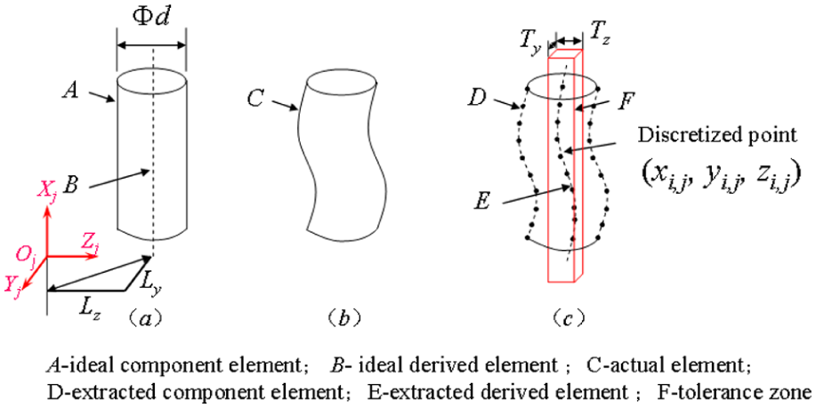
In order to well reflect the variation in every geometrical feature, the parts’ geometrical features are also represented by discrete points in this article, as shown in equation (1), where M is the discrete description of a geometrical feature; it can be any geometrical feature such as a plane and the movement track of an axis; i = 1, 2, 3,…, n is the point index; j = 1, 2, 3,… is the index for coordinate system O_jX_jY_jZ_j and x_i,j, y_i,j and z_i,j represent the coordinates of discretized point i in X-, Y- and Z-directions in coordinate system O_jX_jY_jZ_j, respectively

$$M=\left[\begin{array}{cccccc}\hfill x_{1,j}\hfill & \hfill x_{2,j}\hfill & \hfill \cdots \hfill & \hfill x_{i,j}\hfill & \hfill \cdots \hfill & \hfill x_{n,j}\hfill \\ \hfill y_{1,j}\hfill & \hfill y_{2,j}\hfill & \hfill \cdots \hfill & \hfill y_{i,j}\hfill & \hfill \cdots \hfill & \hfill y_{n,j}\hfill \\ \hfill z_{1,j}\hfill & \hfill z_{2,j}\hfill & \hfill \cdots \hfill & \hfill z_{i,j}\hfill & \hfill \cdots \hfill & \hfill z_{n,j}\hfill \\ \hfill 1\hfill & \hfill 1\hfill & \hfill \cdots \hfill & \hfill 1\hfill & \hfill \cdots \hfill & \hfill 1\hfill \end{array}\right]$$

(1)

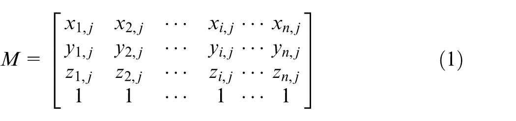
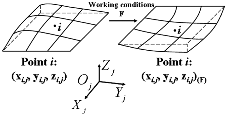
In this article, the main error direction is the vertical direction to the assembly datum surface and is used to search for three highest points. These three points are used to determine the replaced plane of the actual geometrical feature and they have first three coordinate values in the main error direction. Suppose that Z-direction is the main error direction, and z_i,j (i = 1, 2, 3,…, n) can be varied due to factors such as gravity and temperature. As shown in Figure 1, the variation in the geometrical features under actual working conditions can be obtained by combining the discrete points with the variation rule F. By this way, the actual working conditions can be applied to the geometrical feature.

Figure 1.

Variation in the geometrical features under working conditions.

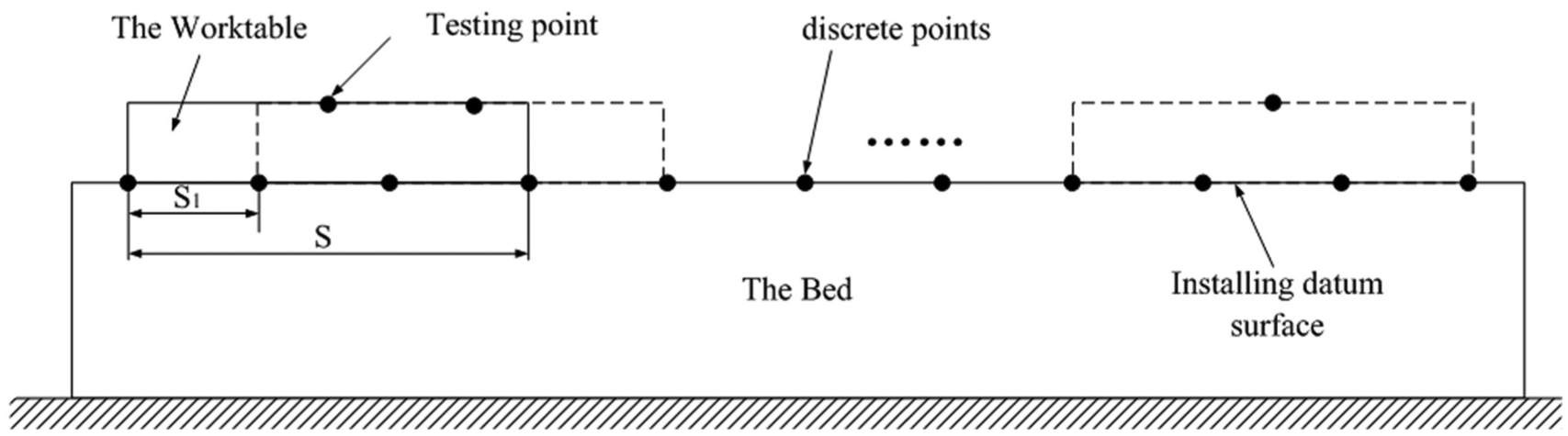
The number of the discrete points can be inferred by testing points. However, there is no reference for testing points. Thus, the number of the testing points on FEs should be determined on-site. Figure 2 and equation (2) show the relationship between the numbers of discrete points and testing points for guideways’ installation datum surfaces. Where n_dp represents the number of the discrete points, n_test represents the number of the testing points, S represents the length of the moving component such as worktable and S₁ represents the distance between two adjacent discrete points. As shown in equation (3), for fixed joint surfaces such as the installation datum surface between the column and bed, the number of discrete points equals to the number of the testing points. In equation (3), n_dp represents the number of the discrete points, and n_test represents the number of the testing points

$$n_{\mathrm{dp}}=2*(n_{\mathrm{test}}+S/S1)$$

(2)

$$n_{\mathrm{dp}}=n_{\mathrm{test}}$$

(3)

Figure 2.

Relationship between the number of the discrete points and the number of the testing points for guideways’ installation datum surfaces.

Mathematical tolerance model

In this article, tolerance analysis in the worst case is derived by combining mathematical tolerance model with the variable dimensional chain. The mathematical tolerance model is not the key point in this article, so only the mathematical model of geometrical tolerances owning rectangular tolerance zone is derived.

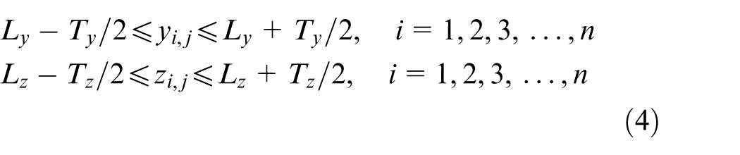
Figure 3 shows a cylinder and the straightness of the cylinder axis is a typical geometrical tolerance owning rectangular tolerance zone. In Figure 3, the actual elements do not coincide with the ideal ones in three-dimensional (3D) case, and the cylinder is discretized as discrete points. In previous tolerance models, the cylinder is acquired by fitting the discrete points. Then the derived elements are obtained to build the mathematical model of tolerance. In this article, the coordinate ranges are limited by inequalities and the tolerance model is then derived. In 3D case, the straightness tolerance of cylinder axis can be expressed by equation (4), where L_y represents the distance of cylinder axis away from plane X_jO_jZ_j; L_z represents the distance of cylinder axis away from plane X_jO_jY_j; T_y represents the tolerance of the straightness of cylinder axis in Y-direction; T_Z represents the tolerance of the straightness of cylinder axis in Z-direction and x_i,j, y_i,j and z_i,j represent the coordinates of discretized point i in X-, Y- and Z-directions in coordinate system O_jX_jY_jZ_j, respectively

$$\begin{array}{c}{L}_y-T_y/2⩽y_{i,j}⩽L_y+T_y/2,i=1,2,3,\dots ,n\hfill \\ L_z-T_z/2⩽z_{i,j}⩽L_z+T_z/2,i=1,2,3,\dots ,n\hfill \end{array}$$

(4)

Figure 3.

Interrelationship of the geometrical feature’s definitions.

Variable dimensional chain under working conditions

Figure 4(a) shows the traditional dimensional chain and the variation in the dimensional chain of a precision horizontal machining center, where the straightness of X-axis motion is a very important precision index. As shown in Figure 4(a), A_Σ in the whole stroke can satisfy the tolerance requirement in ideal conditions. However, the geometrical features will change due to the gravity of components in the whole stroke, and the deviation at position ② has exceeded the tolerance of FR. So it is necessary to construct the variable dimensional chain.

Figure 4.

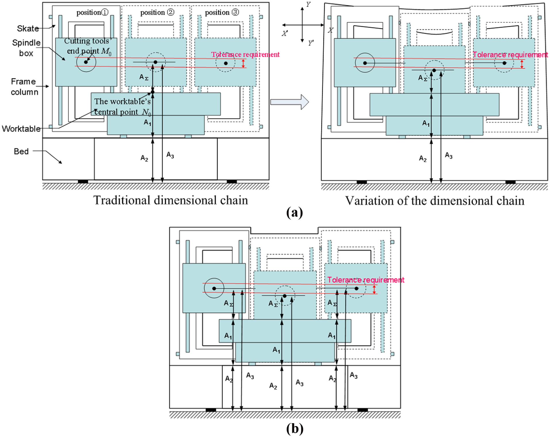
Variation in the deviation stack-up function under working conditions and the variation dimensional chain: (a) the deviation stack-up function of mechanical assemblies along the whole machining stroke under gravity condition and (b) the deviation stack-up function of mechanical assemblies along the whole machining stroke achieved by the method in this article.

When testing the straightness, relative dimensions in several testing points are used as equivalence. So the assembly dimension chain of the straightness could be replaced by several linear dimensional chains as shown in Figure 4(b). A_Σ is the distance between the spindle axis and the working table, A₁ is the distance between upper and lower surfaces of the working table, A₂ is the distance between the upper surface of bed and the ground datum and A₃ is the distance between the spindle axis and the ground datum. The dimension chain of other geometrical tolerances can also be replaced by several linear dimensional chains because that relative dimensions in several testing points are used as equivalence when testing those geometrical deviations.

Variable dimensional chain of mechanical assemblies

Assumptions

The following assumptions are given before establishing the variable dimensional chain:τ

1. Two assembly parts are in contact with each other in three highest points of the discrete coordinate points characterizing the geometrical feature of the part.

2. In the actual measurement, the dimension of FR at a fixed position is regarded as constant, but it varies at different positions in the whole machining stroke.

Coordinate transformation matrix K_ij between two assembly parts

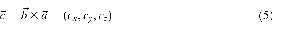
The dimensions of the FR are calculated via transformation matrix. So the most important thing in this model is the calculation of the transformation matrix K_ij. The first step is to find three highest non-collinear points in equation (1). Suppose their coordinates are (x_l, y_l, z_l), (x_m, y_m, z_m) and (x_n, y_n, z_n) respectively; thus, two vectors can be expressed as follows

$$\begin{array}{c}\overrightarrow{a}=(x_l-x_n,y_l-y_n,z_l-z_n)\hfill \\ \overrightarrow{b}=(x_m-x_n,y_m-y_n,z_m-z_n)\hfill \end{array}$$

Plane P₀₁ is determined by these three points. Once vectors $\overrightarrow{a}$ and $\overrightarrow{b}$ are known, the normal vector of the plane P₀₁ ( $\overrightarrow{c}$ ) is calculated according to the right-hand rule. Vector $\overrightarrow{c}$ has the same direction as axis O_jZ_j in the coordinate system O_iX_iY_iZ_i

$$\overrightarrow{c}=\overrightarrow{b}\times \overrightarrow{a}=(c_x,c_y,c_z)$$

(5)

Although the position of plane P₀₁ in the coordinate system O_iX_iY_iZ_i is determined, the worktable can still be rotated or moved within the plane. Therefore, in order to determine the only position of the coordinate system O_jX_jY_jZ_j, the actual assembly constraints should be taken into account. Because the guideway is in close contact with the vertical datum surface, O_jY_j can only have a small angle with O_iY_i. Searching for two points in the three highest points, which have approximately the same Y value. With the assumption that these two points are (x_m, y_m, z_m) and (x_n, y_n, z_n), and y_m > y_n, the vector in the same direction as axis O_jY_j in the coordinate system O_iX_iY_iZ_i can be derived, as shown in equation (6). And then the vector in the same direction as axis O_jX_j can be deduced, as shown in equation (7)

$$\overrightarrow{b}\prime =(x_m-x_n,y_m-y_n,z_m-z_n)=(b_x,b_y,b_z)$$

(6)

$$\overrightarrow{a}\prime =\overrightarrow{c}\times \overrightarrow{b}\prime =(a_x,a_y,a_z)$$

(7)

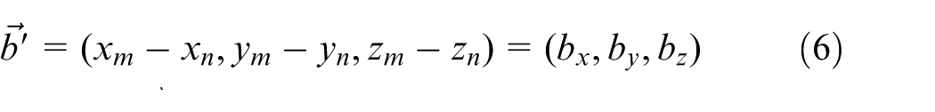
The three vectors in equations (5)–(7) have the same direction as the three axes of O_jX_jY_jZ_j in the coordinate system O_iX_iY_iZ_i. The coordinate transformation matrix between two assembly parts is thus derived as

$$K_{\mathrm{ij}}=\left[\begin{array}{cccc}\hfill k_{11}\hfill & \hfill k_{12}\hfill & \hfill k_{13}\hfill & \hfill k_l\hfill \\ \hfill k_{21}\hfill & \hfill k_{22}\hfill & \hfill k_{23}\hfill & \hfill k_m\hfill \\ \hfill k_{31}\hfill & \hfill k_{32}\hfill & \hfill k_{33}\hfill & \hfill k_n\hfill \\ \hfill 0\hfill & \hfill 0\hfill & \hfill 0\hfill & \hfill 1\hfill \end{array}\right]$$

(8)

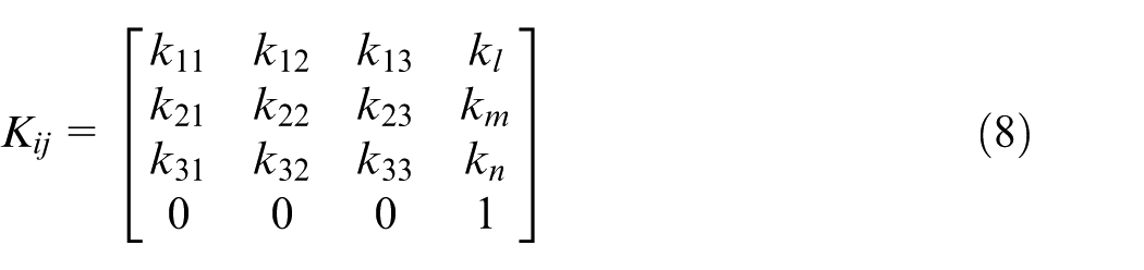
where k₁₁, k₂₁ and k₃₁ are the direction cosines of vector $\overrightarrow{a}\prime$ ; k₁₂, k₂₂ and k₃₂ are the direction cosines of vector $\overrightarrow{b}\prime$ ; k₁₃, k₂₃ and k₃₃ are the direction cosines of vector $\overrightarrow{c}$ ; k_l, k_m and k_n are the origin coordinates of O_jX_jY_jZ_j in the coordinate system O_iX_iY_iZ_i.

Variable dimensional chain

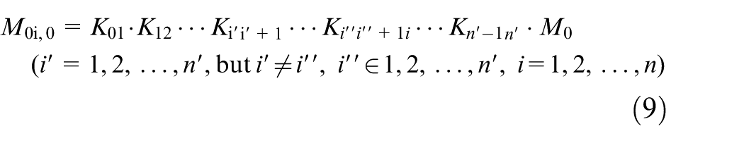
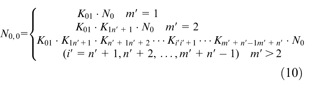
Figure 5 shows the topological structure of a stroke-related mechanical assembly. There are two related geometrical features of two parts (part n′ and part m′ + n′) when referring to a tolerance of FR. The two geometrical features are discretized as M in equation (1), and they are supposed as matrices M₀ (on part n′) and N₀ (on part m′ + n′). Given the assumption that part i″ and i″ + 1 are stroke-related, K₀₁, K_1n′+1, K_i′i′+1 (i′ = 1, 2, 3,…, m′ + n′) and K_i″i″+1i (i″ ∈ 1, 2, 3,…, n′, i = 1, 2,…, n) can be deduced by the calculating process of equations (5)–(7). And then the coordinates of point sets M₀ and N₀ in the coordinate system O₀X₀Y₀Z₀ can be calculated by equations (9) and (10), where M_0i,0 is the coordinate of point set M₀ in the coordinate system O₀X₀Y₀Z₀ when part i″ + 1 moves to the ith position on part i″; N_0,0 is the coordinate of point set N₀ in the coordinate system O₀X₀Y₀Z₀; K_i′i′+1 (i ′= 0, 1, 2, 3,…, m′ + n′) is the transformation matrix between O_i′X_i′Y_i′Z_i′ and O_i′+1X_i′+1Y_i′+1Z_i′+1; K_1n′+1 is the transformation matrix between O₁X₁Y₁Z₁ and O_n′+1X_n′+1Y_n′+1Z_n′+1; K_i″i″+1i (i″ ∈ 1, 2, 3,…, n′, i = 1, 2,…, n) is the transformation matrix between O_i″X_i″Y_i″Z_i″ and O_i″+1X_i″+1Y_i″+1Z_i″+1 when part i″ + 1 moves to the ith position on part i″; n represents that there are n positions in the whole machining stroke.

$$\begin{array}{l}{M}_{0\mathrm{i},0}=K_{01}·K_{12}\cdots K_{\mathrm{i}\prime \mathrm{i}\prime +1}\cdots K_{i″i″+1i}\cdots K_{n\prime -1n\prime }·M_0\\ (i\prime =1,2,\dots ,n\prime ,\mathrm{but}i\prime \ne i″,i″\in 1,2,\dots ,n\prime ,i=1,2,\dots ,n)\end{array}$$

(9)

$$N_{0,0}=\{\begin{array}{l}{K}_{01}·N_{0}m\prime =1\\ K_{01}·K_{1n\prime +1}·N_{0}m\prime =2\\ K_{01}·K_{1n\prime +1}·K_{n\prime +1n\prime +2}\cdots K_{i\prime i\prime +1}\cdots K_{m\prime +n\prime -1m\prime +n\prime }·N_0\\ (i\prime =n\prime +1,n\prime +2,\dots ,m\prime +n\prime -1)m\prime >2\end{array}$$

(10)

Figure 5.

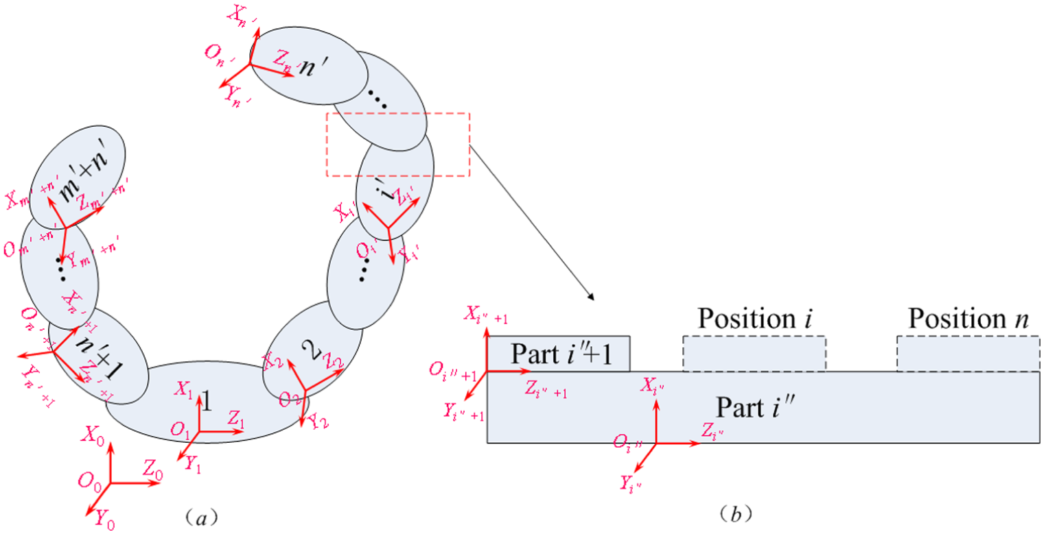
Topological structure of a stroke-related mechanical assembly.

With the assumption that geometrical feature of part m′ + n′ is the measuring datum of FR’s deviation, the deviation stack-up function between the deviations of FEs and FR can be derived by equations (9) and (10). The deviations induced by working conditions include systematic deviations and random deviations. Systematic deviations bring about the position variations in the tolerance zones. The random deviations lead to the variation in FEs in a certain range and eventually cause the deviation of FR varied in a certain range. ²⁴

Tolerance analysis based on the variable dimensional chain

Worst-case method

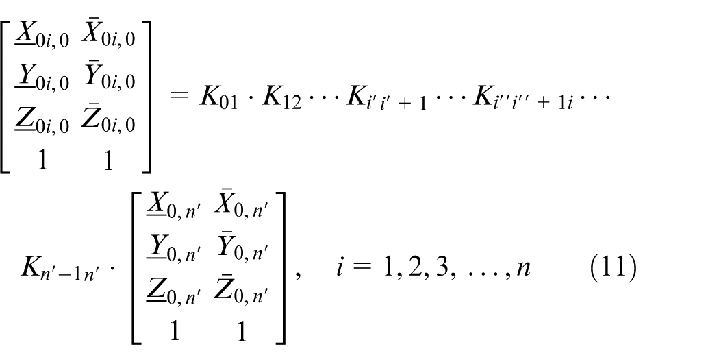
Tolerance analysis in worst case can be acquired by combining equation (9) with the mathematical tolerance model in this article, as shown in equation (11). The deviation variation range of the FR can be derived by equation (11), where ( ${\underset{¯}{X}}_{0,n\prime },{\underset{¯}{Y}}_{0,n\prime },{\underset{¯}{Z}}_{0,n\prime }$ )^T and ( ${\overline{X}}_{0,n\prime },{\overline{Y}}_{0,n\prime },{\overline{Z}}_{0,n\prime }$ )^T are the lower and upper limits of the coordinates of M₀, respectively, and they can be calculated by equation (4); ( ${\underset{¯}{X}}_{0,i,0},{\underset{¯}{Y}}_{0,i,0},{\underset{¯}{Z}}_{0,i,0}$ )^T and ( ${\overline{X}}_{0,i,0},{\overline{Y}}_{0,i,0},{\overline{Z}}_{0,i,0}$ )^T are the lower and upper limits of the coordinates of M_0i,0(X_0i,0, Y_0i,0, Z_0i,0)^T, respectively; n represents that there are n positions in the whole machining stroke

$$\begin{array}{c}\left[\begin{array}{c}\hfill {\underset{¯}{X}}_{0i,0}\hfill \\ \hfill {\underset{¯}{Y}}_{0i,0}\hfill \\ \hfill {\underset{¯}{Z}}_{0i,0}\hfill \\ \hfill 1\hfill \end{array}\begin{array}{c}\hfill {\overline{X}}_{0i,0}\hfill \\ \hfill {\overline{Y}}_{0i,0}\hfill \\ \hfill {\overline{Z}}_{0i,0}\hfill \\ \hfill 1\hfill \end{array}\right]=K_{01}·K_{12}\cdots {K_{i\prime }}_{i\prime +1}\cdots K_{i″i″+1i}\cdots \hfill \\ {K_{n\prime -1}}_{n\prime }·\left[\begin{array}{c}\hfill {\underset{¯}{X}}_{0,n\prime }\hfill \\ \hfill {\underset{¯}{Y}}_{0,n\prime }\hfill \\ \hfill {\underset{¯}{Z}}_{0,n\prime }\hfill \\ \hfill 1\hfill \end{array}\begin{array}{c}\hfill {\overline{X}}_{0,n\prime }\hfill \\ \hfill {\overline{Y}}_{0,n\prime }\hfill \\ \hfill {\overline{Z}}_{0,n\prime }\hfill \\ \hfill 1\hfill \end{array}\right],i=1,2,3,\dots ,n(11)\hfill \end{array}$$

(11)

Monte Carlo simulation method

The tolerance analysis method is obtained by combining the variable dimensional chain with Monte Carlo simulation method. M₀ can be obtained by sampling according to part’s tolerance and its probability distribution. Combined with the deformations under working conditions, the transformation matrices K₀₁, K_1n′+1, K_i′i′+1 (i′ = 1, 2, 3,…, m′ + n′) and K_i″i″+1i (i″ ∈ 1, 2, 3,…, n′, i = 1, 2,…, n) can be deduced by equations (5)–(7). And then the deviation of FR can be acquired by equations (9) and (10). When the sampling process is repeated, the deviation variation range and probability distribution of FR can be derived, and then the tolerance accumulative effect between the tolerances of FEs and FR can be obtained.

Experimental verification

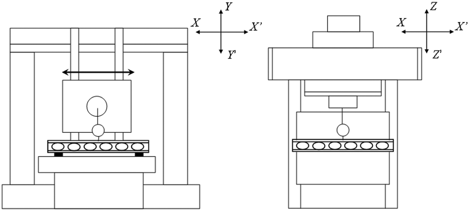
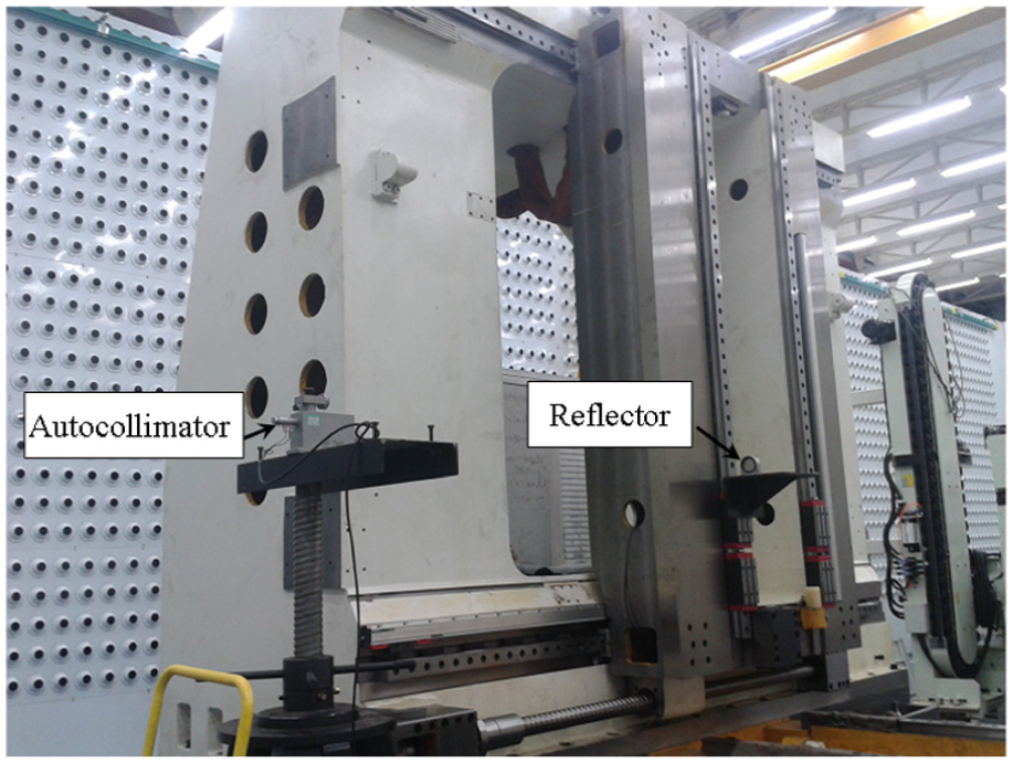
Figure 6 is a horizontal machining center and its simplified schematic diagram. The variable dimensional chain of the straightness of X-axis motion is constructed on the horizontal machining center. Figure 7 shows four parts used to construct variable dimensional chain of the straightness and the coordinate systems of “bed–column–skate–spindle box” are built in Figure 7.

Figure 6.

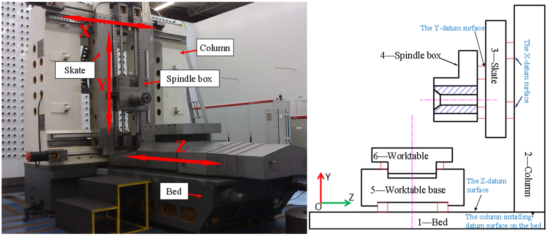
A horizontal machining center and its simplified schematic diagram.

Figure 7.

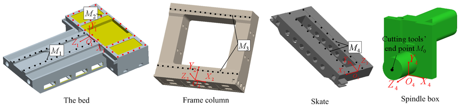
Set of the coordinate systems of “bed, column, skate and spindle box.”

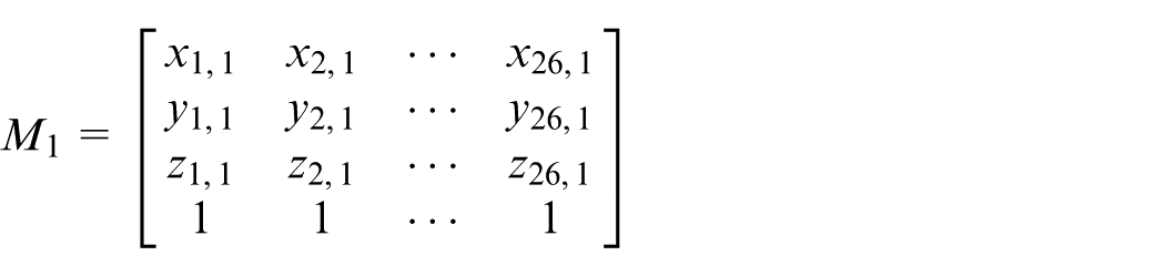
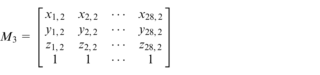
Then the geometrical features of the four parts in Figure 7 are represented as discrete points as shown in equation (1). In Figure 7, M₁ is the discrete description of Z-axis guideways’ installation datum surface on the bed (the Z-datum surface), M₂ is the discrete description of column installation datum surface on the bed; M₃ is the discrete description of X-axis guideways’ installation datum surface on the column (the X-datum surface) and M₄ is the discrete description of Y-axis guideways’ installation datum surface on the skate (the Y-datum surface), respectively. For M₁ to M₄, the naming rule is the same with equation (1).

For M₁, n_test equals to 10, S equals to 0.9 m, S₁ equals to 0.3 m, so the number of the discrete points equals to 26 according to equation (2). Then M₁ is represented as

$$M_1=\left[\begin{array}{cccc}\hfill x_{1,1}\hfill & \hfill x_{2,1}\hfill & \hfill \cdots \hfill & \hfill x_{26,1}\hfill \\ \hfill y_{1,1}\hfill & \hfill y_{2,1}\hfill & \hfill \cdots \hfill & \hfill y_{26,1}\hfill \\ \hfill z_{1,1}\hfill & \hfill z_{2,1}\hfill & \hfill \cdots \hfill & \hfill z_{26,1}\hfill \\ \hfill 1\hfill & \hfill 1\hfill & \hfill \cdots \hfill & \hfill 1\hfill \end{array}\right]$$

For M₂, n_test equals to 20, so the number of the discrete points equals to 20 according to equation (3). Then M₂ is represented as

$$M_2=\left[\begin{array}{cccc}\hfill x_{27,1}\hfill & \hfill x_{28,1}\hfill & \hfill \cdots \hfill & \hfill x_{46,1}\hfill \\ \hfill y_{27,1}\hfill & \hfill y_{28,1}\hfill & \hfill \cdots \hfill & \hfill y_{46,1}\hfill \\ \hfill z_{27,1}\hfill & \hfill z_{28,1}\hfill & \hfill \cdots \hfill & \hfill z_{46,1}\hfill \\ \hfill 1\hfill & \hfill 1\hfill & \hfill \cdots \hfill & \hfill 1\hfill \end{array}\right]$$

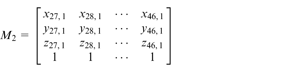
For M₃, n_test equals to 11, S equals to 0.9 m, S₁ equals to 0.3 m, so the number of the discrete points equals to 28 according to equation (2). Then M₃ is represented as

$$M_3=\left[\begin{array}{cccc}\hfill x_{1,2}\hfill & \hfill x_{2,2}\hfill & \hfill \cdots \hfill & \hfill x_{28,2}\hfill \\ \hfill y_{1,2}\hfill & \hfill y_{2,2}\hfill & \hfill \cdots \hfill & \hfill y_{28,2}\hfill \\ \hfill z_{1,2}\hfill & \hfill z_{2,2}\hfill & \hfill \cdots \hfill & \hfill z_{28,2}\hfill \\ \hfill 1\hfill & \hfill 1\hfill & \hfill \cdots \hfill & \hfill 1\hfill \end{array}\right]$$

For M₄, n_test equals to 8, S equals to 0.6 m, S₁ equals to 0.3 m, so the number of the discrete points equals to 20 according to equation (2). Then M₄ is represented as

$$M_4=\left[\begin{array}{cccc}\hfill x_{1,3}\hfill & \hfill x_{2,3}\hfill & \hfill \cdots \hfill & \hfill x_{20,3}\hfill \\ \hfill y_{1,3}\hfill & \hfill y_{2,3}\hfill & \hfill \cdots \hfill & \hfill y_{20,3}\hfill \\ \hfill z_{1,3}\hfill & \hfill z_{2,3}\hfill & \hfill \cdots \hfill & \hfill z_{20,3}\hfill \\ \hfill 1\hfill & \hfill 1\hfill & \hfill \cdots \hfill & \hfill 1\hfill \end{array}\right]$$

Necessity of constructing the variable dimensional chain

In this section, the variation value of the dimensional chain due to gravity deformation is used to verify the necessity of constructing the variable dimensional chain. The measurement theory of the straightness of X-axis motion is shown in Figure 8, and the dimensional chain of the straightness of the X-axis motion under gravity is established by equations (9) and (10).

Figure 8.

Measuring theory of the straightness of X-axis motion.

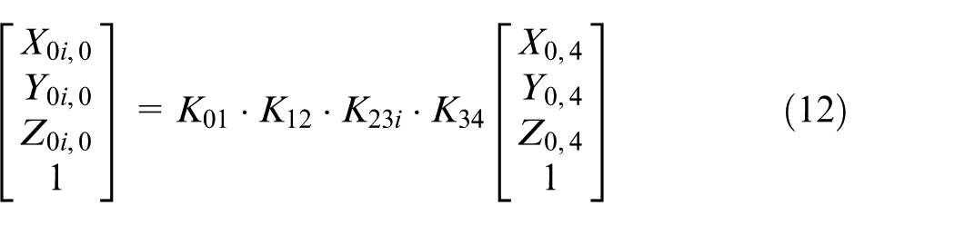
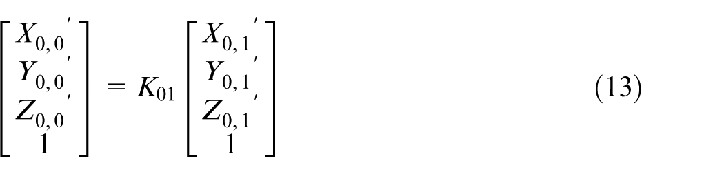
In equations (9) and (10), m′ equals to 1, n′ equals to 4, n equals to 9 and i″ equals to 2 for the horizontal machining center in Figure 6. Then K₀₁, K₁₂, K_23i and K₃₄ can be obtained by equations (5)–(7). And M_0i,0 can be acquired by equations (9) and (10), which is shown in equations (12) and (13), where (X_0,4, Y_0,4, Z_0,4)^T and (X_0,1′, Y_0,1′, Z_0,1′)^T are the coordinates of points M₀ and N₀ in O₄X₄Y₄Z₄ and O₁X₁Y₁Z₁; (X_0i,0, Y_0i,0, Z_0i,0)^T are the coordinates of M₀ in O₀X₀Y₀Z₀ when the skate is at ith position on the frame column; (X_0,0′, Y_0,0′, Z_0,0′)^T are the coordinates of point N₀ in O₀X₀Y₀Z₀; K₀₁ represents the transformation matrix between O₀X₀Y₀Z₀ and O₁X₁Y₁Z₁, and K₁₂ and K₃₄ can be deduced the rest from this; K_23i represents the transformation matrix between O₂X₂Y₂Z₂ and O₃X₃Y₃Z₃ at position i

$$\left[\begin{array}{c}\hfill X_{0i,0}\hfill \\ \hfill Y_{0i,0}\hfill \\ \hfill Z_{0i,0}\hfill \\ \hfill 1\hfill \end{array}\right]=K_{01}·K_{12}·K_{23i}·K_{34}\left[\begin{array}{c}\hfill X_{0,4}\hfill \\ \hfill Y_{0,4}\hfill \\ \hfill Z_{0,4}\hfill \\ \hfill 1\hfill \end{array}\right]$$

(12)

$$\left[\begin{array}{c}\hfill {X_{0,0}}^{\prime }\hfill \\ \hfill {Y_{0,0}}^{\prime }\hfill \\ \hfill {Z_{0,0}}^{\prime }\hfill \\ \hfill 1\hfill \end{array}\right]=K_{01}\left[\begin{array}{c}\hfill {X_{0,1}}^{\prime }\hfill \\ \hfill {Y_{0,1}}^{\prime }\hfill \\ \hfill {Z_{0,1}}^{\prime }\hfill \\ \hfill 1\hfill \end{array}\right]$$

(13)

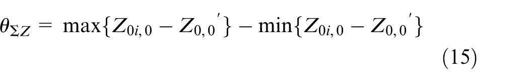
Then the straightness of the X-axis motion in Y- and Z-directions can be calculated with equations (14) and (15). Equations (14) and (15) are the deviation stack-up functions between the dimensional or geometrical deviations of FEs and FR

$${\theta }_{\Sigma Y}=max\{Y_{0i,0}-{Y_{0,0}}^{\prime }\}-min\{Y_{0i,0}-{Y_{0,0}}^{\prime }\}$$

(14)

$${\theta }_{\Sigma Z}=max\{Z_{0i,0}-{Z_{0,0}}^{\prime }\}-min\{Z_{0i,0}-{Z_{0,0}}^{\prime }\}$$

(15)

The value of A₁ plus A₂ is regarded as constant because the leveling ruler on the worktable is treated as the measuring datum when measuring the straightness of the X-axis motion. Hence, the geometrical features M₁, M₂ and M₄ are treated as ideal and K₀₁, K₁₂ and K₃₄ are only translation matrices. K_23i can be calculated by M₃ and M₃ is acquired as follows.

The variation in the straightness of the X-axis motion is mainly caused by the deformation of the X-axis datum surface. Using finite element simulation software Samcef V8.1, the deformations of the 28 discretized coordinates on the datum surface of the column were calculated by simulating the gravity deformations at nine positions in the whole machining stroke. The results are shown in Table 1. In Table 1, the values of “UP-Z direction” at 300, 500,…, 2900 mm represent the variation values of z_1,2, z_2,2,…, z_14,2 in M₃; the values of “DOWN-Z direction” at 300, 500,…, 2900 mm represent the variation values of z_15,2, z_16,2,…, z_28,2 in M₃; the values of “UP-Y direction” at 300, 500,…, 2900 mm represent the variation values of y_1,2, y_2,2,…, y_14,2 in M₃; the values of “DOWN-Z direction” at 300, 500,…, 2900 mm represent the variation values of y_15,2, y_16,2,…, y_28,2 in M₃, and in M₃, x_1,2, x_2,2,…, x_14,2 equal to 300, 500,…, 2900 mm. x_15,2, x_16,2,…, x_28,2 equal to 300, 500,…, 2900 mm, respectively.

Table 1.

Deformations of the 28 discretized coordinates on the datum surface (µm).

	300	500	700	900	1100	1300	1500
UP-Z direction	−41.8	−42.8	−39.4	−36.5	−35.4	−36.0	−35.8
UP-Y direction	23.8	28.7	36.7	44.8	50.7	54.7	55.7
DOWN-Z direction	−1.1	−0.3	−0.1	−0.4	−0.2	−0.1	−0.1
DOWN-Y direction	4.1	4.5	3.5	2.6	2.3	2.4	2.9
	1700	1900	2100	2300	2500	2700	2900
UP-Z direction	−38.3	−35.6	−35.5	−35.8	−36.1	−40.2	−42.7
UP-Y direction	56.9	54.9	53.0	48.3	41.4	33.2	26.6
DOWN-Z direction	0.4	−0.3	−0.3	−0.1	−0.6	0	−0.7
DOWN-Y direction	2.8	2.6	2.8	2.9	2.9	4.2	5.0

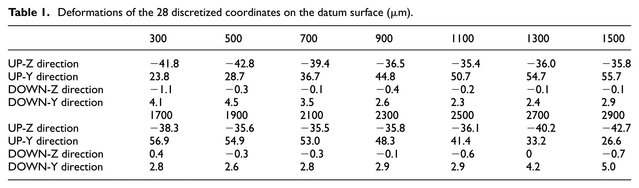
Table 1 shows the variation values of M₃ when only the gravity deformation of the machine tools is considered. Then K_23i (i = 1, 2, 3,…, 9) can be calculated by equations (5)–(7). Set the cutting tools’ end point as M₀ (0, 0, 200, 1)^T and the worktable’s central point as N₀ (0, 100, 400, 1)^T. The coordinates of point M_0i,0 at nine positions were calculated by substituting the deformations into equation (12). And the dimension variation in A_Σ can be acquired by the calculated coordinates Y_0i,0(i = 1, 2,…, 9), as shown in Figure 9.

Figure 9.

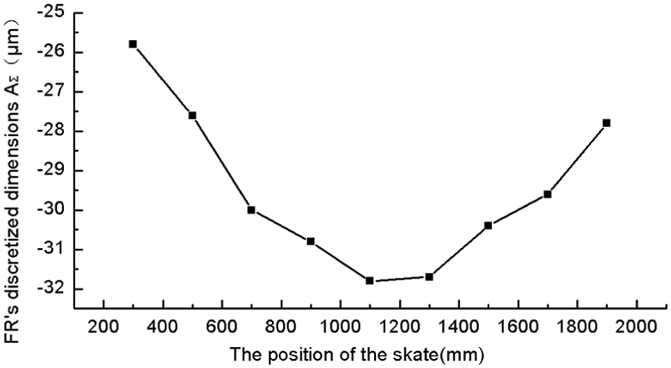
Tolerance position variations in the dimension A_Σ under gravity condition.

In Figure 9, the variation in A_Σ in the whole machining stroke is 6.1 µm. However, the FR of the straightness error is 6 µm, so the variation in the assembly dimensional chain under gravity cannot be ignored.

Calculating accuracy verification of the variable dimensional chain

In this section, all the factors are considered when calculating the variation of the dimensional chain. The calculating process is the same as section “Necessity of constructing the variable dimensional chain.” The variation values of the dimensional chain calculated in this section are compared with the actual measured values to verify the accuracy of the variable dimensional chain.

Experimental verification method

The first group of geometric errors was measured when the assembly process was completed. So the effects of residual stress and material creep can be ignored. The final deformations of the guideway’s surface M₃ can be calculated by equation (16)

$$P_{i,j}={\delta }_{i,j}+\delta {\prime }_i+\frac{i}{13}\delta ″$$

(16)

where P_i,j denotes deformations of the guideway’s surface when the assembly is completed; j (j = 1, 2, 3, 4) represents the deformations of the upper level installing surface (UP-Z direction in Table 1), upper vertical installing surface (UP-Y direction), lower level installing surface (DOWN-Z direction) and lower vertical installing surface (DOWN-Y direction), respectively; δ_i,j represents the simulated deformations of the guideways; δ_i′ represents the scraping amount of the point on the guideway’s surface; δ″ represents the value of the bed level.

The coordinates of point M_0i,0 at nine positions can be obtained by substituting the deformations into the variable dimensional chain. And the straightness of the X-axis motion was measured by autocollimator Angle AIM PRO and its accuracy is 0.5″. Figure 10 shows the measurement principle of the straightness. The calculated errors were compared with the measured ones to verify the accuracy of the variable dimensional chain.

Figure 10.

Measuring theory of the straightness of the X-axis motion.

Results

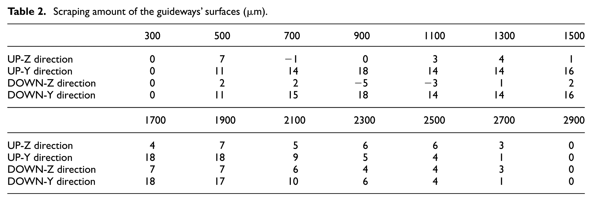
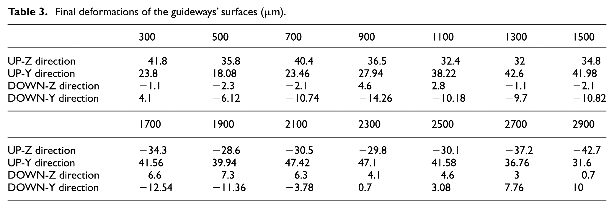
In equation (16), measuring result δ″ was that the right end is 5 µm higher than the left end of the bed. The scraping amount δ_i′ is shown in Table 2. The final deformations of the guideways’ surfaces (M₃) were calculated when the assembly was completed, as shown in Table 3.

Table 2.

Scraping amount of the guideways’ surfaces (µm).

	300	500	700	900	1100	1300	1500
UP-Z direction	0	7	−1	0	3	4	1
UP-Y direction	0	11	14	18	14	14	16
DOWN-Z direction	0	2	2	−5	−3	1	2
DOWN-Y direction	0	11	15	18	14	14	16
	1700	1900	2100	2300	2500	2700	2900
UP-Z direction	4	7	5	6	6	3	0
UP-Y direction	18	18	9	5	4	1	0
DOWN-Z direction	7	7	6	4	4	3	0
DOWN-Y direction	18	17	10	6	4	1	0

Table 3.

Final deformations of the guideways’ surfaces (µm).

	300	500	700	900	1100	1300	1500
UP-Z direction	−41.8	−35.8	−40.4	−36.5	−32.4	−32	−34.8
UP-Y direction	23.8	18.08	23.46	27.94	38.22	42.6	41.98
DOWN-Z direction	−1.1	−2.3	−2.1	4.6	2.8	−1.1	−2.1
DOWN-Y direction	4.1	−6.12	−10.74	−14.26	−10.18	−9.7	−10.82
	1700	1900	2100	2300	2500	2700	2900
UP-Z direction	−34.3	−28.6	−30.5	−29.8	−30.1	−37.2	−42.7
UP-Y direction	41.56	39.94	47.42	47.1	41.58	36.76	31.6
DOWN-Z direction	−6.6	−7.3	−6.3	−4.1	−4.6	−3	−0.7
DOWN-Y direction	−12.54	−11.36	−3.78	0.7	3.08	7.76	10

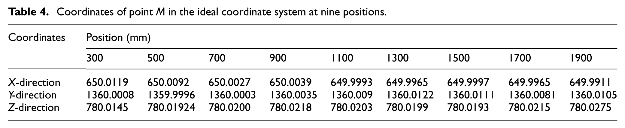
The coordinates of point M_0i,0 at nine positions were obtained by substituting the deformations in Table 3 into equation (12), and the results are shown in Table 4. And then the straightness of the X-axis motion in planes XOZ and XOY is calculated by equations (15) and (14).

Table 4.

Coordinates of point M in the ideal coordinate system at nine positions.

Coordinates	Position (mm)
	300	500	700	900	1100	1300	1500	1700	1900
X-direction	650.0119	650.0092	650.0027	650.0039	649.9993	649.9965	649.9997	649.9965	649.9911
Y-direction	1360.0008	1359.9996	1360.0003	1360.0035	1360.009	1360.0122	1360.0111	1360.0081	1360.0105
Z-direction	780.0145	780.01924	780.0200	780.0218	780.0203	780.0199	780.0193	780.0215	780.0275

The deformation data in Table 3 are actually the deformations of the discretized points used to characterize the guideways’ surfaces M₃. Hence, the discretized points can be fitted into a plane, and the HTM can be derived, which has the same calculating process as equations (5)–(7).

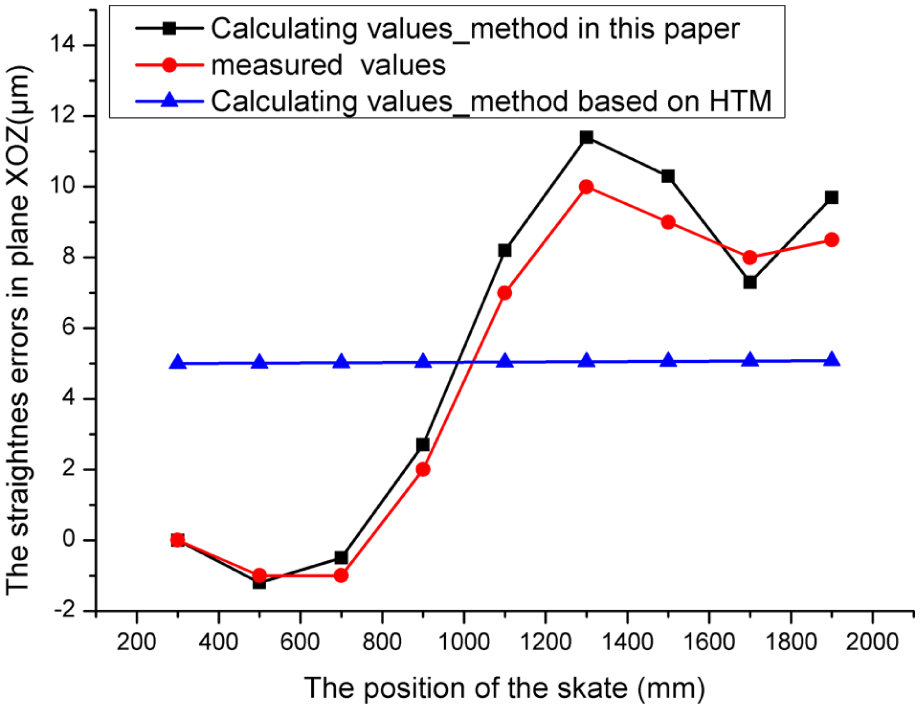
Straightness of the X-axis motion in plane XOZ

As shown in Figure 11, the straightness of the X-axis motion in plane XOZ calculated by the variable dimensional chain is 13.0 µm, while the measured value is 12 µm. The calculated errors by the model in this article and the measured results are approximately the same and the largest deviation is 1 µm at testing point 8, while the calculated errors by HTM method have a big difference compared with the measured results and the largest deviation is 6 µm.

Figure 11.

Straightness of the X-axis motion in plane XOZ calculated by the variation dimensional chain in this article and the measured one.

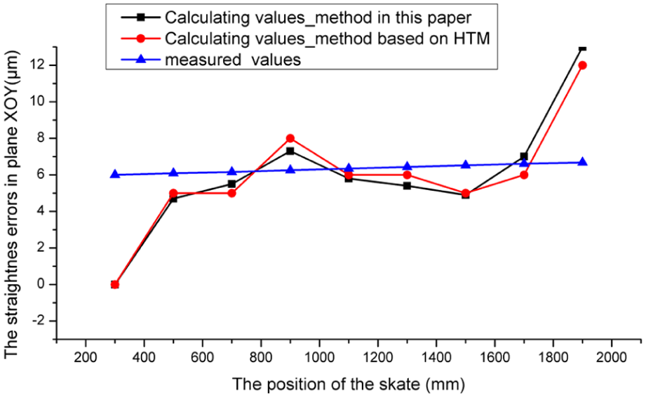
Straightness of the X-axis motion in plane XOY

As shown in Figure 12, the straightness of the X-axis motion in plane XOY calculated by the variable dimensional chain in this article is 11.4 µm, while the measured value is 10 µm. The calculated errors by the model in this article and the measured results are approximately the same and the largest deviation is 1.4 µm at testing point 6, while the calculated errors by HTM method have a big difference with the measured results and the largest deviation is 5 µm. The accuracy of the variable dimensional chain of calculating the dimensional or geometrical error of FR had been verified.

Figure 12.

Straightness of the X-axis motion in plane XOY calculated by the variation dimensional chain in this article and the measured one.

Tolerance analysis using Monte Carlo simulation method

The new tolerance analysis method combines the variable dimensional chain with Monte Carlo simulation method, which has been described in section “Monte Carlo simulation method.” Section “Necessity of constructing the variable dimensional chain” is actually a one-time calculating process of tolerance analysis. When the calculating process is repeated, the deviation variation range and probability distribution of FR can be derived.

The coordinates of M₃ without considering the gravity deformation can be acquired as follows: the straightness tolerances of the guideway’s datum surfaces were transformed as a set of coordinate points according to the tolerance model. Because the coordinate point obeys a certain probability distribution in the whole variation zone, the coordinates of M₃ can be acquired by randomly selecting coordinates, according to the probability distribution of the coordinate point.

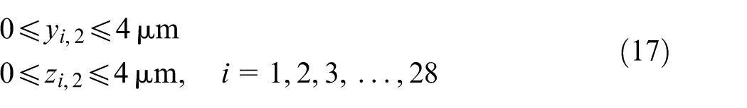
In the design stage, the straightness values of the X-axis guideway in the planes XOY and XOZ are all 4 µm, and both of them obey a normal distribution. Then the variation range of the coordinates in M₃ can be represented as equation (17) according to equation (4)

$$\begin{array}{c}0⩽y_{i,2}⩽4\mu \mathrm{m}\hfill \\ 0⩽z_{i,2}⩽4\mu \mathrm{m},i=1,2,3,\dots ,28\hfill \end{array}$$

(17)

The deformation values of the guideways can be obtained by adding the randomly selected coordinates with the deformations of the guideways in Table 1. The coordinate transformation matrices were calculated by equations (5)–(7). Here, K_23i is the rotation matrix, while K₁₂ and K₃₄ are the translation matrices. Based on these, one calculation process of calculating the coordinates of point M_0i,0 is completed by equations (14) and (15). Repeating the sampling process, the variation range and the distribution of the straightness of the X-axis motion in two directions were calculated under the condition that the sampling times are 100,000. The calculating results are shown in Figure 13(a)–(d), which show the situations considering and not considering the effect of the gravities of mechanical assemblies.

Figure 13.

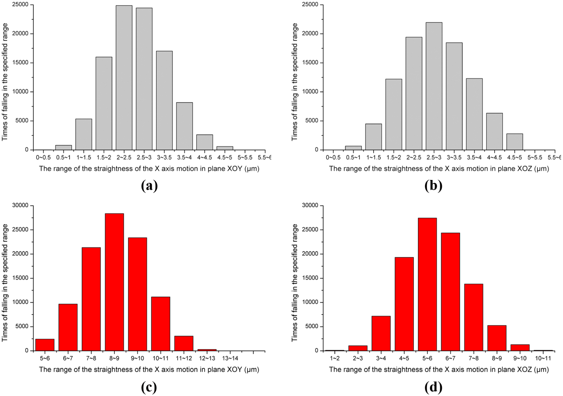
Probability distribution of the straightness of the X-axis motion: (a) the probability distribution of the straightness of the X-axis motion in Y-direction without considering the gravity, (b) the probability distribution of the straightness of the X-axis motion in Z-direction without considering the gravity, (c) the probability distribution of the straightness of the X-axis motion in Y-direction considering the gravity and (d) the probability distribution of the straightness of the X-axis motion in Z-direction considering the gravity.

The FRs of the straightness of the X-axis motion in two directions are both 6 µm. Comparing with Figure 13, the assembly successful rates of the straightness of X-axis motion in Y- and Z-directions were 99.96% and 100% when the effects of the components’ gravities were not considered, while the assembly successful rates were 2.43% and 55.13% if the gravities of the mechanical assemblies were considered. In this article, the effect of gravity on the tolerance analysis was analyzed, and the results show that the actual working conditions cannot be ignored in tolerance design.

Discussion

1. This article takes a horizontal machining center as an example to study the variable dimensional chain. The variation in the dimensional chain under gravity deformation was considered. The location or size of the tolerance of FR is influenced by the variation value of the dimensional chain induced by the actual working conditions. The variation value is either equal to or far greater than the tolerance of FR, so the variation in the dimensional chain has a significant influence on the tolerance allocation results and cannot be ignored in tolerance design. Based on the variable dimensional chain proposed, the tolerance analysis results were acquired on a horizontal machining center when the effects of the components’ gravities were considered and not considered. The results show that without considering the effect of gravity, the assembly successful rates of the straightness of X-axis motion in Y- and Z-directions were 99.96% and 100%, respectively, while the assembly successful rates were 2.43% and 55.13% when considering the gravity of the mechanical assemblies. Conclusion can thus be drawn that the actual working conditions have a great influence on the tolerance analysis results and cannot be ignored.

2. An experiment is carried out to verify the accuracy of the calculation results. The straightness errors of X-axis motion were calculated with the model presented in this article and the model based on HTM. The two calculating results were compared with the measured results. It can be seen that the calculation result based on HTM method was maximally 6 µm different from the measured value, a large gap than that of the calculation result based on the model proposed in this article. The reason lies in that the form deviation of the geometrical feature is ignored in the model based on HTM. The results show that the deviation stack-up function constructed by variable dimensional chain is more accurate than the method based on HTM.

3. Machine tool is typically a stroke-related mechanical assembly, and many components are associated with stroke, such as the bed component and the column component. Hence, it is necessary to construct the variable dimensional chain for stroke-related mechanical assembly. Deviation stack-up function which takes stroke as the independent variable is constructed via variable dimensional chain. With the variable dimensional chain proposed in the article, reasonable tolerance allocation under working conditions can be obtained.

Conclusion

This article presents a variable dimensional chain, which can reflect the variation in the dimensional chain under working conditions for stroke-related mechanical assemblies. The variable value of the dimensional chain will significantly influence the tolerance allocation results. Some conclusions can be drawn as follows:

1. The location or size of the FR’s tolerance is significantly influenced by the variation in the dimensional chain induced by the actual working conditions, so the variation in the dimensional chain must be considered at the tolerance design stage. This article takes a horizontal machining center as the example to study the variable dimensional chain. The variation in the dimensional chain under gravity deformation was considered. The results show that the actual working conditions have a great influence on the tolerance analysis results and cannot be ignored.

2. An experiment was carried out to verify the accuracy of the variable dimensional chain. The results show that deviation stack-up function constructed by variable dimensional chain is more accurate than the method based on HTM for stroke-related mechanical assemblies.

3. The application object of the variable dimensional chain is stroke-related mechanical assembly such as machine tools. Accurate deviation stack-up function that takes stroke as the independent variable is constructed via variable dimensional chain. With the variable dimensional chain proposed in the article, reasonable tolerance allocation under working conditions can be obtained.