Sage Journals: Discover world-class research

Abstract

The optimization for multidisciplinary engineering systems is highly complicated, which involves the decomposing of a system into several individual disciplinary subsystems for obtaining optimal solutions. Managing the coupling between subsystems remains a great challenge for global optimization as the existing methods involve inefficient iterative solving processes and thus have higher time cost. Some strategies such as discipline reorder, coupling suspension and coupling ignoring can to some extent reduce the execution cost. However, there are still some deficiencies for these approaches such as uniform handling of the couplings, complete decoupling and heavy burden of system optimizer. To overcome the above drawbacks, a serialization-based partial decoupling approach is proposed in this study, which consists of three main steps. First, different disciplines are clustered into some subsystems by analyzing the interdisciplinary sensitivities. Then, for each subsystem, a serialization process is proposed to ensure no coupling loops exist and the subsystem can be solved with no iteration, which can reduce the time cost for solving the disciplinary problem to a large degree. Finally, a local optimization model is constructed for each subsystem to maintain the scale of the global optimizer and ensure mutual independence and parallel processing. The proposed three-layer framework ensures the feasibility of solving for each subsystem and improves the efficiency of optimization execution. Several experiments have been conducted to demonstrate the effectiveness and feasibility of the proposed approach.

Keywords

Serialization partial decoupling clustering analysis serializable solving local optimization multidisciplinary design optimization

Introduction

The design problems in modern engineering systems generally have a large scale and involve many factors from a number of domains. Therefore, this type of problem is often logically divided into several disciplines by researchers and engineers, each of which is derived from one or more major domains.^1–3 An imperative issue in the case of multidisciplinary design and optimization is to address the unavoidable couplings among these disciplines.^4–6 Thus, the complex couplings and dependencies should be considered to get the optimal solutions during the process of complex system design.^7–9 With the requirements of high computational precision for highly complex design problems, the traditional theories of complex system design have evident limitations as they have no consideration of interdisciplinary couplings. Multidisciplinary design optimization (MDO)^10–12 is a hot research field in recent years in which the interdisciplinary couplings are considered to construct high-fidelity models of complex problems during the early analysis phase.^13–15 However, how to solve MDO problems efficiently is still a great challenge. A lot of research has been conducted to develop efficient and feasible decoupling strategies for MDO problems.^16,17

Several general-purpose optimization methods have been proposed for MDO problems in engineering.^18,19 Sobieszezanski-Sobieski²⁰ did pioneering working in this field and proposed a solving method based on sensitivity. The core idea is to consider the effects among the disciplines concerned at each time of iteration. Several years later, a new architecture was proposed based on the concept of subspace. These two ideas are considered as the foundation of this field. The current state-of-the-art work related to the MDO architecture can be classified into two main types, namely, single-level optimizer and bi-level optimizer. The former contains multidisciplinary feasible (MDF), individual discipline feasible (IDF) and all at once (AAO).

Specifically, MDF is a basic architecture, which consists of a global optimizer and a uniform system solver. The optimizer manages optimization task while the solver is responsible for analyzing the disciplines involved in the solving process. The global optimizer provides values of design variables that are used as the inputs for the solver. The coupling variables in the system are solved through lots of complete iterative computations. This architecture does not change the global optimization model. However, a complete interdisciplinary analysis is required and the computational cost is generally expensive. IDF avoids the iterative interdisciplinary analysis by adding the coupling variables as global design variables and some constraints of the global optimization model. The result is that the search space has been decreased and the computation time of the global optimizer has increased. AAO is based on IDF and further decreases the complexity of the analysis process. The state variables in different disciplines are also added into the global optimizer, and thus, the search space is further decreased. The architectures with two levels of optimizers based on decomposition strategy contain collaborative optimization (CO), concurrent system synthesis optimization (CSSO)²¹ and bi-level integrated system synthesis (BLISS).²² The complex optimization problems are hierarchically decomposed into several sub-problems when these approaches are adopted, each of which constructs a local optimizer to deal with its corresponding sub-problems and processes its own design variables and constraints. The main problems of two-level optimizer architectures include the following: (1) the local optimizers are not synchronous and thus, the global optimizer cannot be executed unless all the local optimizers are completed, which affects the whole optimization performance; (2) data should be exchanged between the global optimizer and all the local optimizers, and thus, a lot of data exchange operations are needed and (3) the statistical techniques and gradient information are required, which is a great challenge for constructing an efficient and effective local optimization model for a complex multidisciplinary system.

It can be seen from the above analysis that even though considerable work has been done on MDO, there still exist some deficiencies for the existing approaches. First, they decompose all the disciplines in a uniform way. In fact, for a multidisciplinary system consisting of a large number of disciplines, the degrees of coupling between different disciplines are quite different and thus, they should be dealt with differently. Second, for the tightly coupled disciplines with some bidirectional couplings, decoupling them completely may lead to intensive computation. Finally, the computational burden of the global optimizer is heavy as it needs to process too much information. In this sense, how to handle the decoupling variables with a localized way in which only the corresponding subsystem is related should be considered.

In this study, a serialization-based partial decoupling (SPD) method is proposed to tackle the decoupling problem. The process of SPD method mainly consists of three steps. First, several disciplines of a system are clustered into some subsystems based on the coupling sensitivity, that is, each subsystem is made up of several disciplines. Second, a serialization operation is executed for partial decoupling between subsystems by removing the coupling loops in an efficient manner. Finally, a local optimization model is constructed and executed to maintain the consistency of the decoupling variables for each subsystem. The most primary mechanism of SPD is that only a small percentage of coupling variables are required to be decoupled and no iterative solving is required for these coupling variables. Therefore, the global optimization solving process is efficient whereas the solving accuracy is acceptable.

This article is organized as follows. Section “Overview of the SPD method” describes the flowchart and architecture of the proposed SPD method. Section “Clustering analysis based on sensitivity” presents the clustering process based on degree of coupling between different disciplines. In sections “Decoupling of a subsystem” and “ Local optimization in a subsystem,” the decoupling process in a subsystem and the local optimization process are detailed, respectively. The whole approach is demonstrated and evaluated using three experiments introduced in section “Computational experiments.” Finally, some conclusions and discussions are given in section “Conclusion and future work.”

Overview of the SPD method

Compared to the existing architectures, the most obvious feature of the SPD method is that it contains three layers of components: the global optimizer on the top, the subsystem solver in the middle and the local optimizer on the bottom. Data are transferred among the three layers of components in a specific order. The main advantages of the proposed SPD method include the following: (1) the coupling variables that need to be decoupled have been decreased to a great extent by introducing the subsystem mechanism since the number of tasks to be processed is less than that of the traditional approaches; (2) a balance in the scales of different subsystems is attained using the clustering analysis strategy for the coupling variables, which ensures that the time cost for solving each subsystem will not be much different and (3) only one local optimizer is constructed for each subsystem in order to control the complexity of local optimization problem, which can be constructed automatically and solved in an efficient way. Meanwhile, no additional dependent variables are required on the global optimizer, which ensures high solution efficiency.

SPD flowchart

As mentioned above, the core idea of the SPD method is to conduct data transfer and problem solving based on the three-layer architecture. In each time of iteration, the clustering analysis operation is executed on the whole coupling system and several subsystems are generated. Bidirectional interactions are conducted between the global optimizer and the subsystems while data are transferred in a unidirectional way within each subsystem. The SPD flowchart for solving MDO problems is given in Figure 1, which starts with system initialization by setting the global design variables, the local design variables for each discipline and the interdisciplinary coupling variables. For the sake of clarity, a number of terms are used in this study: the coupling variable decoupled among the subsystems is called the global decoupling coupling variable (GDCV); the coupling variable decoupled in one subsystem is called the local decoupling coupling variable (LDCV) and the coupling variable without being decoupled at time of each iteration is called the reserved coupling variable (RCV).

Figure 1.

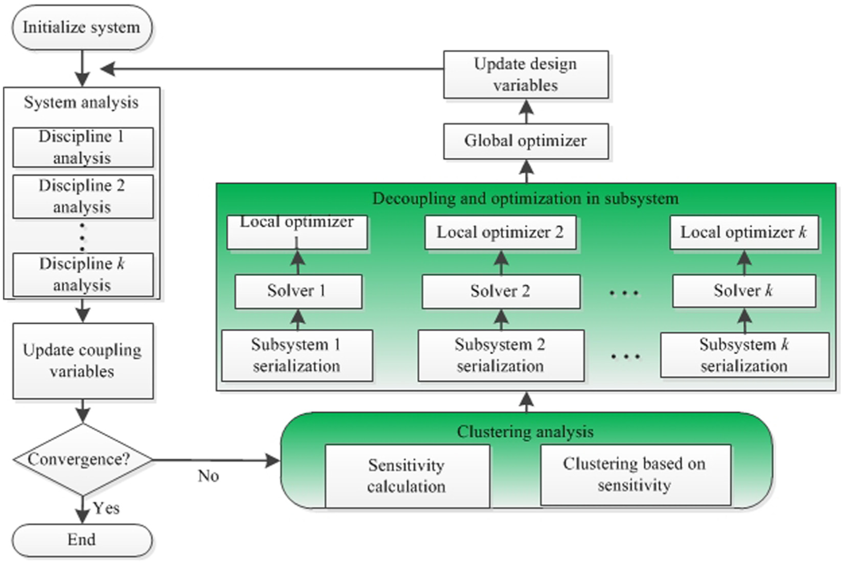
Flowchart of SPD.

After the system is initialized, four main steps need to be taken in the method:

Disciplinary analysis: conducting the disciplinary analysis for each discipline and updating the output variables.

Clustering analysis: executing the multidisciplinary clustering analysis as follows:

Calculating the sensitivity values between each discipline and each global optimization objective.

Conducting the clustering analysis based on the sensitivity value and then some subsystems are obtained. At the same time, adding the corresponding constraints of GDCVs to the global optimizer to attain coupling consistency among subsystems.

Subsystem optimization: optimizing all the subsystems as follows:

Executing the serialization operation in each subsystem.

Analyzing the subsystem and solving each output variable in the subsystem in a sequence according to the directed graph structure.

Conducting the local optimization operation for the whole LDCVs in each subsystem.

Global optimization: optimizing the whole system globally and generating the new design variable values.

Step 2 is repeated until the optimization process converges or the largest number of iteration has been reached.

SPD framework

The framework of SPD is shown in Figure 2. It can be seen that there are three layers in the SPD framework. Specifically, the top level is the global optimizer managing the optimization of global objectives and the middle level is the subsystem solver that is responsible for the internal decoupling and discipline analysis. The bottom level is the local optimizer that is responsible for handling the LDCVs that need to be decoupled. This clear structure enables reasonable and effective processing on each variable.

Figure 2.

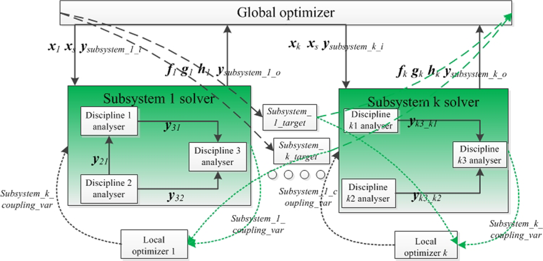
SPD framework.

Such a framework allows the SPD method to have the advantages of concurrent analysis and design while in the MDF architectures each subsystem only has one solver. Similar to those in IDF, the interactions between the global optimizer and each subsystem in SPD contain both design variables and the decoupling variables among subsystems. The global optimizer serves the purpose of coordinating the subsystems through these interactive coupling variables. Therefore, the subsystems are independent of each other and in this case, parallel computing techniques can be applied.

The global optimizer selects the local design variables x _k, the global design variables x _s and the coupling variables y _{subsystem_k_i} among the subsystems as the inputs for each subsystem. Each subsystem sends the objective values f _k, the constraint values g _k, h _k and coupling values y _{subsystem_k_o} back to the global optimizer as the outputs. These variables are represented as black solid line between the global optimizer and the subsystem solvers. It should be noted that each subsystem has a large number of coupling variables such as y ₃₁, y ₃₂ and y ₂₁ shown in black lines in subsystem 1. To deal with the coupling variables in the subsystems, additional target variables are added into the global optimizer and the latter delivers the target variables to each local optimizer according to the dependency relationships. For instance, the target variable Subsystem_1_target is delivered to local optimizer k in green dashed line. Meanwhile, the local optimizer delivers the dependent coupling variables to the subsystem such as Subsystem_k_coupling_var in black dashed line. Because of the unidirectional depending structure of the coupling variables in the subsystem, the disciplines in a subsystem can be solved according to its dependency relationships, which can ensure that the analysis process is executed only one time and can thus decrease the data transfer between the components to a great extent.

Based on the above analysis, the advantages of this framework can be summarized as follows. First, the number of final subsystems is far less than the disciplines after executing the clustering analysis. Therefore, the number of local optimizers required is pretty small. Second, each subsystem can be analyzed rapidly through the serialization operation since only one time of analysis is required. Specifically, the differences between SPD and other traditional architectures are as follows:

Compared to MDF, although some constraints are added for SPD in the search space, it is unnecessary to conduct iterative multidisciplinary analysis at the subsystem level. The execution efficiency can be improved, which is important for the coupling situations with more loops.

Compared to IDF, the coupling variables that SPD needs to process is much less, most of which remain unchanged. It is a target decoupling strategy, and thus the number of constraints added into the search space is far less than that of IDF. As a result, the scale of the global optimizer will not increase greatly. In this sense, it is more flexible in the search space and more satisfactory solutions can be acquired.

Compared to the architectures with bi-level optimizers, the most outstanding advantage of SPD is that the number of local optimizers decreases a lot by constructing the subsystem components efficiently and reasonably. Meanwhile, the rapid subsystem analysis is executed and thus, the efficiency of solving for all the subsystems is improved as a whole.

Clustering analysis based on sensitivity

The degree of coupling among the disciplines involved and the global objective is calculated in this study, which is called coupling sensitivity. The existing approaches pay little attention to coupling sensitivity and often ignore some connotative information. With regard to SPD, a combination of the coupling sensitivity and a clustering strategy is adopted, that is, a multidisciplinary system is clustered into several subsystems according to the coupling sensitivity values obtained. Each subsystem may contain one or several disciplines and execute data transfer with the global optimizer. It is noteworthy that the subsystems are independent of each other and thus, they can be executed simultaneously.

Sensitivity analysis

In MDO, sensitivity analysis refers to the analysis of system performance by evaluating its degree of being sensitive due to the changes in design variables or parameters. By performing in-depth analysis of the sensitivity information, the impacts of system design variables on the objectives or constraints can be identified. The coupling value between the subsystems can also be determined.

The sensitivity between a design function and a design variable represents the degree of the changes in the design function caused by the changes in the design variable at a specific point, which can be described using the partial derivatives of the function. At a specific design point $X_{P}$ , the sensitivity of the design function $φ_{i} (X)$ with respect to a specific design variable $x_{j}$ is thus defined as follows

S_{ij} = \frac{\partial φ_{i} (X)}{\partial x_{j}} |_{X = X_{P}}, i = 1, 2, \dots, m, j = 1, 2, \dots, n

(1)

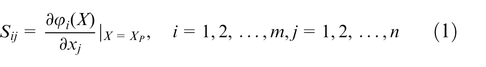
In this expression, m and n are the numbers of design functions and design variables, respectively. The larger the value of $| S_{ij} |$ , the more sensitive the design function $φ_{i} (X)$ with respect to $x_{j}$ , that is, $x_{j}$ has a larger impact on $φ_{i} (X)$ . $S_{ij}$ represents the monotonicity of function $φ_{i} (X)$ with respect to variable $x_{j}$ . If $S_{ij} < 0$ , it means that $φ_{i} (X)$ is monotonically decreasing with respect to $x_{j}$ . Otherwise, it is monotonically increasing. Therefore, the sensitivity value expresses two kinds of information: monotonicity and degree of being sensitive.²³

The sensitivity of design function $| S_{ij} |$ is employed to define the degree of coupling. The larger the value of $| S_{ij} |$ , the stronger the coupling degree.

Subsystem clustering based on sensitivity

The idea that a complex engineering system is divided into several subsystems can be regarded as an abstract description of the problem using smaller and more manageable sub-problems. Each discipline contains local variables, global variables, output variables and its dependent input variables from other disciplines. The input variables from other disciplines are the interdisciplinary coupling variables. Two rules are mainly considered when the clustering analysis is conducted. First, the subsystem coupling degree should be as low as possible, that is, decreasing the dependencies between subsystems as much as possible. Also, there are no additional constraints for the coupling degree inside one subsystem. Second, the coupling degree between any subsystem and the global objective should be as low as possible. In this way, it can be ensured that the impacts of each subsystem with regard to the global objective are uniform and balanced. The traditional clustering problems usually involve several features, that is, the dimension of each point and its values are represented on the absolute coordinate system. However, the distances between a point and the other points are known for the clustering problems based on sensitivities among the disciplines, which can be considered as a representation based on the relative coordinate system. Based on the above analysis, the initial centroid must belong to the current point set. In this study, an adapted K-means clustering algorithm is proposed to minimize the sum of the distances in each cluster. Obviously, different subsystem partitions lead to different decoupling variables, and thus have large impacts on the final subsystem sensitivities. To maximize the sensitivities among all the subsystems, it is represented as follows

E = \frac{\sum_{i = 1}^{M} \sum_{j = 1}^{N} \sum_{k = 1}^{P} S_{jk}^{i}}{M}

(2)

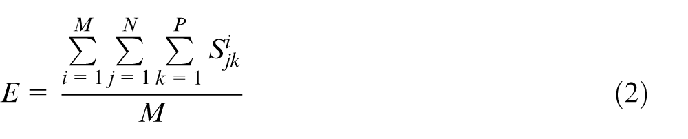
Specifically, E represents the average subsystem sensitivities; M and N are the numbers of subsystems and disciplines, respectively; P is the number of disciplines in each subsystem. It can be seen that the representation is simple and can precisely reflect the distance between the subsystems compared to the standard distance measure used in the traditional K-means method. The adopted clustering strategy in this study is K-means algorithm combined with the global objective. Suppose that the allowed time of iteration is T, then the clustering process is as follows:

Calculate the sum of global objective sensitivities with respect to all the coupling variables at the kth time of iteration and mark it as S. The global objective sensitivity with respect to each subsystem is then S/M, represented as AvgS. Construct a container with M elements, in which each element records the global objective sensitivity (with an initial value of 0) with respect to each subsystem. Select M points whose sensitivities with respect to other points are not the largest as the initial centroids to ensure that the final result is not the worst.

For each left point x_i in the point set, calculate its sensitivity with respect to all the subsystems and select the subsystem with the biggest value. At the same time, calculate the corresponding global objective sensitivity value in the container. If it is bigger than AvgS, abandon the current selection and consider the subsystem with the second best sensitivity.

Calculate the current subsystem sensitivity value and re-allocate new centroids.

Repeat Steps 2 and 3 until k reaches the maximal number of allowed iteration T, or the condition $‖ E^{(k)} - E^{(k - 1)} ‖ < Δ$ is satisfied.

The selection of initial centroids has a large impact on the final clustering result in clustering algorithms. In this study, the selection strategy can to some extent ensure that good quality can be achieved for the final result. The reason for this is that for the problems in this study, the number of disciplines is not too large and thus, the number of clustering points is not large.

Decoupling of a subsystem

After the clustering operation is conducted, each subsystem is highly correlated as several coupling loops exist. To improve the subsystem solving efficiency, SPD is executed to remove the internal coupling using the strategy of loop removal in a directed graph and serialize the disciplines in a subsystem. After that, the solver for the subsystem can execute the analysis process in an efficient way without the need of conducting iteration.

Connection path between disciplines

A subsystem is composed of one or more disciplines after the clustering analysis, in which the disciplines are highly correlated and dependent on each other. There may be several coupling variables with a large coupling degree in each subsystem. Moreover, it is also possible that there is a number of coupling loops in a subsystem. It is time-consuming to perform analysis for each subsystem during an optimization process. In this study, not all the couplings between the disciplines are considered to be decoupled. Only a part of them with lower coupling values are considered to serialize all the disciplines in the same subsystem to solve the subsystem in a serializable way without the need of conducting iteration. Based on the above analysis, a loop removal method in directed graphs is adapted in this study with its details explained in the next paragraph.

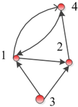
Each discipline is regarded as a vertex in the directed graph-based representation of a subsystem. The coupling variable between two disciplines means there exists one dependency and can be regarded as one directed edge. As shown in Figure 3, two edges exist between discipline 1 and discipline 4, which means there are bidirectional couplings between these two disciplines. The output variables of discipline 4 are required when discipline 1 is analyzed and vice versa. If there is a directed path between A and B in a directed graph, there exists a connection path between A and B. The number of this kind of directed paths is called the degree of a connection path. As shown in Figure 3, no connection path exists from discipline 4 to discipline 3 whereas there is a connection path from discipline 3 to discipline 4 and the degree of connection path is 3. Specifically, three directed paths exist, namely, 3 → 1 → 4, 3 → 2 → 4 and 3 → 1 → 2 → 4.

Figure 3.

An example of connection paths.

SPD process in a subsystem

General process of partial decoupling based on serialization

In this study, the breadth-first search method is used to conduct the serialization process. A list called vertex state list (VSL) is required to record the states of vertexes in the directed graph. The sensitivity analysis information is taken into consideration when an edge is required to be removed in a loop, that is, the edge with the weakest sensitivity is removed so as to decrease the total influence to the largest extent. The input for this algorithm is a directed graph with loops while its output is a directed graph with no inner loops. The detailed process is as follows:

Select the vertex with the biggest in-degree as the initial vertex and insert it into the VSL.

Select the next untreated vertex as the current point in the VSL and find all the connection paths from the current vertex to the initial vertex. In addition, the vertexes dependent on the current vertex are also found, which are called dependent vertexes.

For each dependent vertex, insert it into the list if it has not been inserted into the VSL; otherwise, check whether this dependent vertex lies on one or more connection paths. If only one connection path exists, compare the absolute values of the sensitivity of the directed edges and remove the directed edge with the weakest value in order to reserve the strong couplings in the subsystem. Another case is the one having more than one connection paths, that is, the number of coupling loops is more than one. In this case, all the shared edges need to be found out and the one with weakest sensitivity absolute value should be removed. Only one edge is required to be removed through this strategy and all the coupling loops involved are broken.

Repeat Steps 2 and 3 until all the vertexes in the VSL are processed.

Formal demonstration of loop removal

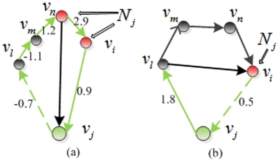
To provide a formal demonstration of the effectiveness of the SPD approach, the mathematical reasoning process is given as follows. Suppose that there is a directed graph G, marked as G = (V, A), which is composed by a non-null limited vertex set V and some ordered pair set A. Each element of $V = {v_{1}, v_{2}, \dots, v_{n}}$ is called a vertex of G. Another set $A = {a_{1}, a_{2}, \dots, a_{m}}$ is called the edge set of G. Each element $a_{ij} = (v_{i}, v_{j})$ is called the edge from vertex $v_{i}$ to vertex $v_{j}$ , which corresponds to a coupling relationship in a real system. Additionally, $N_{i}$ represents the neighbor vertex set depending on $v_{i}$ , from which there exists one edge pointing to $v_{i}$ .

A directed loop is a loop whose edges have the same direction. This characteristic can ensure that it can be judged whether there is one directed loop correctly combining the proposed strategy between two vertexes. Figure 4 shows the formal demonstration of loop removal with two cases, in which green vertex is the current processed object, red vertices are its neighbors, black vertices are involved objects. These vertices are connected by directed edges. The mathematical reasoning process of loop removal between vertexes $v_{i}$ and $v_{j}$ is as follows:

$v_{i}$ has already been processed whereas $v_{j}$ has not, as shown in Figure 4(a). Moreover, there is not one edge from $v_{j}$ to $v_{i}$ , which means $v_{j}$ does not depend on $v_{i}$ . At this moment, it cannot be concluded that no directed loop exists containing vertexes $v_{i}$ and $v_{j}$ .

When $v_{j}$ becomes the vertex currently processed as indicated with green color, its neighbor vertexes can be obtained, that is, $N_{j}$ that consists of vertexes $v_{n}$ and $v_{i}$ both indicated with red color in Figure 4(a). This means that vertexes $v_{i}$ and $v_{n}$ alike are connected to $v_{j}$ with an edge element $a_{ij}$ . Vertex $v_{i}$ will be processed as a dependency vertex of $v_{j}$ .

Finally, one (the case in Figure 4(a)) or more (the case in Figure 4(b)) connection paths are found from $v_{j}$ to $v_{i}$ . For the case in Figure 4(a), all the edges involved in the loop are indicated with green color and the edge from $v_{j}$ to $v_{l}$ is removed because of its weakest sensitivity absolute value. Two edges are considered for the case in Figure 4(b) and the shared edge from $v_{i}$ to $v_{j}$ is removed because of its weakest value. It can be seen that if this edge is broken, it can be assured that all the directed loops will be broken. This strategy can break up all the directed loops between the current vertex $v_{j}$ and the element of $N_{j}$ . Furthermore, all the directed loops can be broken up between any two vertexes in G.

Figure 4.

A formal demonstration of loop removal.

Illustration of the whole SPD process

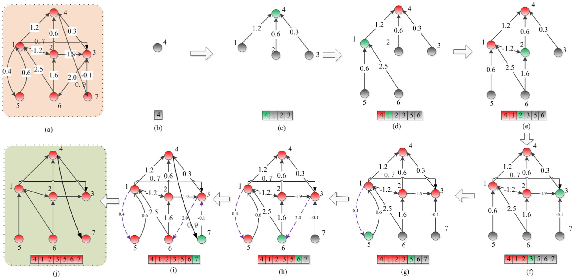
Figure 5 illustrates the algorithm in detail. The elements including the vertices and edges in Figure 5(a) represent one subsystem. The sub-figures from Figure 5(b) to Figure 5(i) presents the algorithm steps for the given example successively. Figure 5(a) shows the algorithm’s inputs which include 7 vertexes and 13 directed edges. In terms of the different colors used, red vertexes are treated, green vertex is the current vertex, gray vertexes are untreated and purple edges are removed edges. The serialized process is detailed as follows:

Select vertex 4 as the initial vertex since it has the biggest in-degree and insert it into the VSL, as shown in Figure 5(b).

Select vertex 4 as the current vertex and find all its dependent vertexes, which are vertexes 1, 2 and 3 in this case. Insert them into the VSL and mark vertex 4 as treated, as shown in Figure 5(c).

Select vertex 1 as the current vertex and insert its dependent vertexes 5 and 6 into the VSL and mark it as treated, as shown in Figure 5(d).

Select vertex 2 as the current vertex which has two dependent vertexes, namely, vertexes 1 and 6. However, they are already in the VSL; it is unnecessary to do the inserting operation again. There is only one connection path from vertex 2 to vertex 4, namely, 2 → 4. Moreover, both vertex 1 and vertex 6 are not in this connection path. The directed edges from these two vertexes to vertex 2 can be added into the directed graph. Mark vertex 2 as treated, as shown in Figure 5(e).

Select vertex 3 as the current vertex, and insert vertex 7 into the VSL. Obviously, there is only one connection path from vertexes 3 to 4, and therefore, the directed edge from vertexes 2 to 3 can be reserved. In addition, vertex 1 depends on vertex 3 and it has already been marked as treated. However, there is no connection path from vertexes 3 to 1, which means no directed loop containing vertexes 3 and 1 exists. Therefore, no edge is required to be removed. Marked vertex 3 as treated, as shown in Figure 5(f).

Select vertex 5 as the current vertex. According to their sensitivity values, the directed edge from vertexes 1 to 5 is removed because of smaller sensitivity values. Marked vertex 5 as treated, as shown in Figure 5(g).

Select vertex 6 as the current vertex. It can be seen that vertex 3 depends on it and there are two connection paths from vertex 6 to vertex 3 (6 → 1 → 2 → 3, 6 → 2 → 3). In this case, the directed edge from vertexes 3 to 6 is removed, resulting in the breaking up of two coupling loops. Mark vertex 6 as treated, as shown in Figure 5(h).

Select vertex 7 as the current vertex. It can be seen that vertex 4 depends on it. However, there is a connection path from vertexes 7 to 4, namely, 7 → 3 → 4. Thus, the directed edge from vertexes 7 to 3 is removed because of its smallest absolute sensitivity value. Mark vertex 7 as treated, as shown in Figure 5(i).

Finally, all the vertexes are treated. Figure 5(j) is the final directed graph obtained as the output of the algorithm.

Figure 5.

Serialization process in a subsystem.

Serializable solving in a subsystem

After the serialization operation is completed, the solution sequence is also determined for each subsystem. The solving algorithm of the serialized directed graph is as follows:

Calculate the out-degree for each vertex in the serialized directed graph.

Find the vertex whose out-degree is 0, put it into the sequence solving list and decrease all of the out-degree of its dependent vertexes by 1.

Repeat Step 2 until all the vertexes have been placed in the solving sequence list.

Take Figure 4(j) as an example; the calculation process is detailed as follows:

The out-degree of vertex 7 is 0; put it in the solving sequence list and decrease the out-degree of vertex 4 by 1.

The out-degree of the initial vertex 4 is 0; put it in the solving sequence list and decrease the out-degree of vertexes 1, 2 and 3 by 1.

The out-degree of vertex 3 is 0; put it in the solving sequence list. Decrease the out-degree of vertexes 1 and 2 by 1.

The out-degree of vertex 2 is 0; thus, it is put in the solving sequence list. Decrease the out-degree of vertexes 1 and 6 by 1.

The out-degrees of vertex 1 is 0 and thus, they are put in the solving sequence list. Decrease the out-degree of vertexes 5 and 6 by 1.

Put vertexes 5 and 6 in the solving sequence list. The final solving sequence list is then obtained as (7-4-3-2-1-6-5). The subsystem solver is executed according to this sequence without the need to perform iteration.

Note that many coupling variables among different disciplines can be reserved using the serialized decoupling strategy. As shown in this example with initial 13 coupling variables, 10 coupling variables are reserved after the subsystem decoupling operation has been executed. The subsequent local optimizer only needs to deal with three decoupled variables. Compared to IDF’s operation of adding 13 constraints to be considered by the global optimizer, the proposed SPD is much more efficient in terms of search space exploration. Moreover, each subsystem solver only runs one time whereas in MDF three iteration-based analysis will be required. This shows that solving efficiency is significantly improved. In particular, for the system with more complicated coupled relationships, the performance improvement achieved by SPD is much more prominent.

Local optimization in a subsystem

As mentioned above, most of the coupling variables can be analyzed serially after the previous step is executed. A small part of variables need to be decoupled. These variables can be regarded as design variables and some corresponding constraints are appended in the global optimization model. However, it will possibly make the global optimization model to be excessively constrained, and as a result the search space is greatly narrowed down.

In this study, a local optimization method is proposed to handle the coupling variables within a subsystem and keep the whole system consistent. In this case, the key issue is how to ensure the efficiency of solving the global optimization model and the acceptance of local dynamical optimization models. Meanwhile, it is also important to deal with the related decoupled variables in a reasonable way. Based on the above analysis, the construction of a proper local optimization model is necessitated. As shown in Figure 6, for each time of iteration, the bottom local optimizer accepts the target variables from the global optimizer and the output variables of its corresponding subsystem. The decoupled variables in each subsystem are regarded as the optimization variables of a local optimization model. Each local optimizer is only conducted for its corresponding subsystem to solve the decoupled variables. Moreover, the coupling sensitivities of the decoupled variables for its corresponding subsystem are also taken into account since different decoupled variables make distinct impacts on the same subsystem. To precisely reflect the impacts on a local optimization model, the coupling sensitivities are calculated and appended to local optimization model. For the local optimization objective, it is the combination of the coupling sensitivities and the square sum of the difference between the decoupled variables and the target variables. The detailed process of constructing the local optimization process for the ith subsystem is as follows:

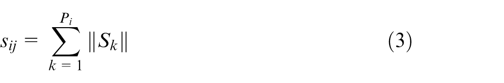
Calculate the sensitivity S_ij for the jth decoupled variable. In equation (3), P_i is the number of coupling variables in the ith subsystem and S_k is the sensitivity between the jth and kth decoupled variable

s_{ij} = \sum_{k = 1}^{P_{i}} ‖ S_{k} ‖

(3)

Normalize the values in the vector S_i and obtain the vector W_i .

Construct the local optimization model using equation (4)

f_{i} = \sum_{j = 1}^{Q_{i}} W_{ij} {({\hat{y}}_{j_t} - y_{j_t})}^{2}

(4)

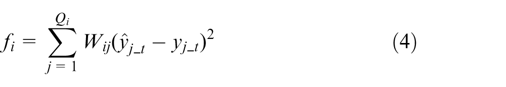
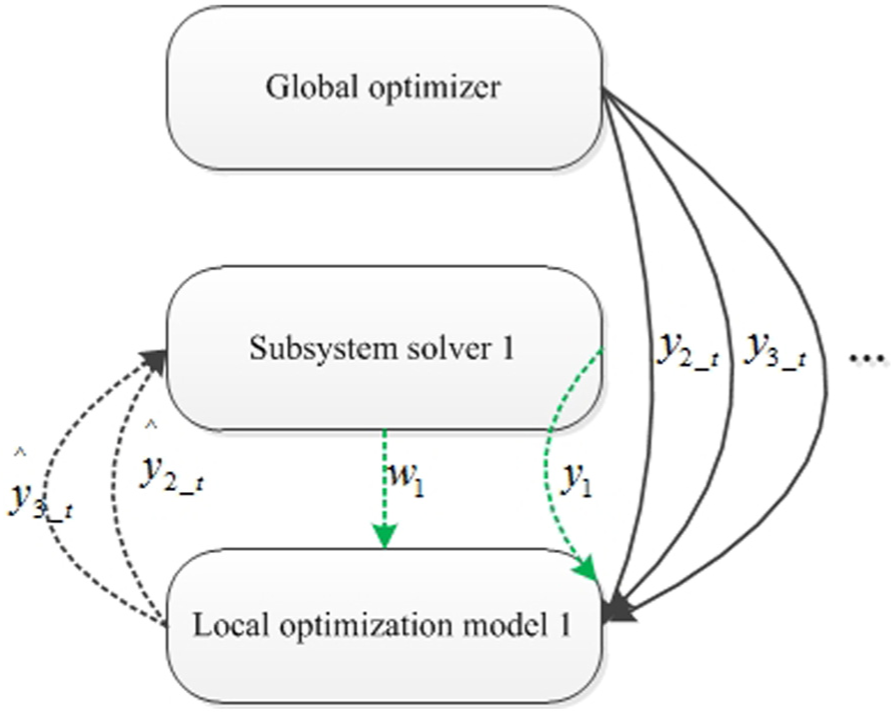
In equation (4), Q_i is the number of decoupled variables in the ith subsystem; y_{j_t} is the target variable delivered from the global optimizer, which is a constant in the local optimization model and ${\hat{y}}_{j_t}$ is the local optimization variables. Some boundaries and local constraints may also be given. According to the characteristics of the local optimization model, the optimization method named square quadratic programming is used.²⁴

Figure 6.

Construction of a local optimization model.

It should be noted that the global optimizer does not operate on the coupling variables in the internal subsystem directly whereas a corresponding target variable is appended. This strategy can ensure the components normally communicate without affecting the flexibility of the global optimizer and in this way search efficiency can be ensured. To avoid long running time caused by the inner loop during the local optimization operation, a maximum number of iteration values can be set.

The advantages of this proposed method include the following: (1) the subsystems can be solved independently and simultaneously since the local optimizer only communicates with its corresponding subsystem; (2) for a decoupled variable in a subsystem, a corresponding target variable is added into the global optimizer, which drives the coupling variables toward the optimal solution. Compared to the handling of inter-subsystem variables, the global optimizer is more flexible and efficient in terms of search space exploration and (3) each subsystem only contains one local optimization model and is dynamically constructed with a fast solving speed. These characteristics can help improve the overall performance.

Computational experiments

To demonstrate the efficacy and efficiency of the proposed SPD approach, three experiments of multidisciplinary optimization are constructed using different mathematical models. These models have some representative features: (1) involving multiple variables, (2) involving multiple disciplines and (3) being highly coupled. Moreover, the optimization results of SPD are compared to MDF and IDF since bi-level structural strategy is not considered in the proposed SPD in this work. The experiments are conducted on the OpenMDAO²⁵ platform developed by NASA.

Partial decoupling of a single subsystem

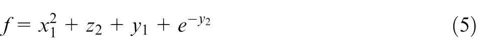
The first typical test application is called the Sellar²⁶ problem which has a mathematical model as follows:

Minimize

f = x_{1}^{2} + z_{2} + y_{1} + e^{- y_{2}}

(5)

Design variables: $x_{1}$ , $z_{1}$ , $z_{2}$

Subject to

y_{1} = z_{1}^{2} + x_{1} + z_{2} - 0.2 y_{2}

y_{2} = \sqrt{y_{1}} + z_{1} + z_{2}

In this example, two disciplines are entirely coupled through $y_{1}$ and $y_{2}$ even it looks simple. It is solved through three architectures, namely, SPD, MDF and IDF. This problem is directly described as one subsystem, and thus, clustering analysis is not required. In the SPD method, $y_{1}$ is decoupled and a local optimizer is constructed to deal with it. This experiment is used to demonstrate the effectiveness of partial decoupling and local optimization.

Table 1 shows the result of Experiment 1. It can be seen that IDF has the optimal result but requires the longest time. On the contrary, MDF’s execution efficiency is better than the others but it has the worst results. The proposed SPD method lies between the two in terms of both efficiency and performance. Moreover, the final two coupling variables converge to the same position. The experimental results indicate that the proposed SPD method has good effectiveness in terms of the partial decoupling strategy.

Table 1.

Results of Experiment 1.

	SPD	IDF	MDF
Optimal positions
z ₁	1.977670	1.977658	1.977639
z ₂	0.0	0.0	0.0
x ₁	0.0	0.0	0.0
Coupling variables
y ₁	3.16	3.16	3.16
y ₂	3.755309	3.755383	3.755278
Optimal f	3.1833932	3.1833914	3.1833937
Runtime (s)	0.555	0.641	0.251

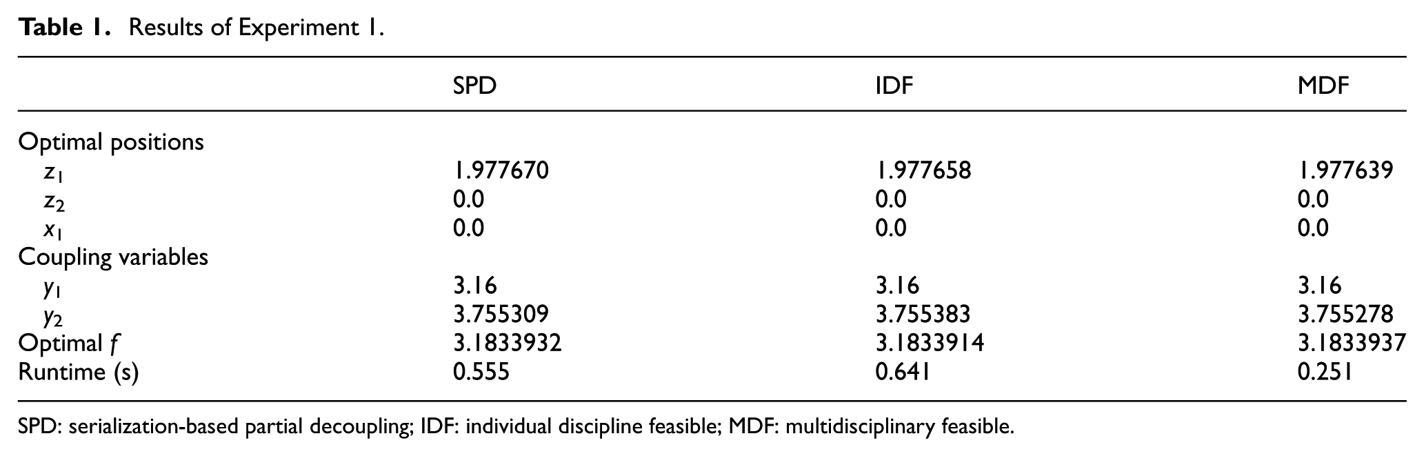
SPD: serialization-based partial decoupling; IDF: individual discipline feasible; MDF: multidisciplinary feasible.

Serializable decoupling of multidisciplinary problems

To demonstrate the clustering analysis and serializable decoupling strategy, a large-scale complicated system is constructed with the help of CASCADE²⁷ and is shown below

Minimize

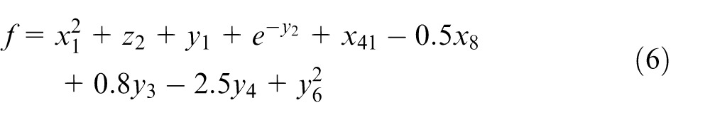
\begin{matrix} f = x_{1}^{2} + z_{2} + y_{1} + e^{- y_{2}} + x_{41} - 0.5 x_{8} \\ + 0.8 y_{3} - 2.5 y_{4} + y_{6}^{2} \end{matrix}

(6)

Design variables: x ₁, x ₃, x ₄₁, x ₄₂, x ₅, x ₈, z ₁, z ₂

Subject to

y_{1} = z_{1}^{2} + x_{1} + z_{2} - 0.2 y_{2}

y_{2} = \sqrt{y_{1}} + z_{1} + z_{2}

y_{3} = z_{1} + z_{2}^{3} + x_{3} - 0.5 y_{1} + 2 y_{5}

y_{4} = z_{2} - x_{41} + 0.5 x_{42} + y_{1}^{2} - y_{3}

y_{5} = z_{1} + z_{2} - x_{5} + \sqrt{y_{2}} + 2.5 y_{3} + y_{7}

y_{6} = z_{1} - y_{4}^{2} + y_{8}

y_{7} = z_{1} - z_{2} + y_{1} + 0.2 y_{6} - 3 y_{9}

y_{8} = z_{1} + z_{2} - x_{8} + 1.5 y_{2} + \sqrt{y_{5}}

y_{9} = z_{1} + y_{4}

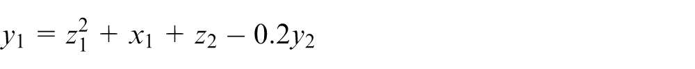
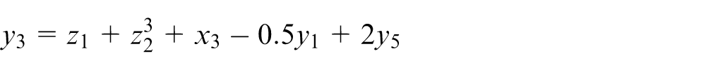
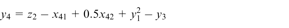
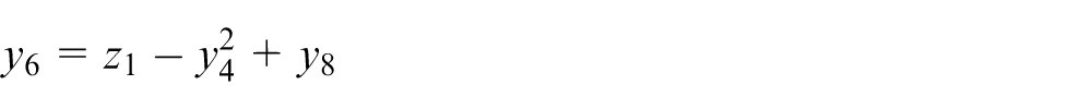
This optimization problem is composed of two global design variables, eight local design variables, two global constraints, nine logical disciplines and 17 coupling variables. Figure 7 gives the design structure matrix of this problem to help more clearly understand the coupling relationships and sequences. It can be seen that each discipline has one output variable in this case.

Figure 7.

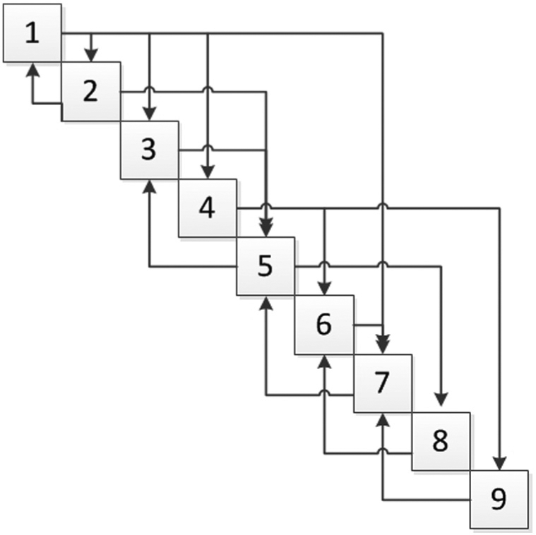
Design structure matrix of the case in Experiment 2.

The numerical calculation process in this experiment converged within nine times of iteration, with the numbers of GDCVs, LDCVs and RCVs changing dynamically for each time of iteration. Figure 8 shows the changes in the quantities of these variables. It can be seen that the values of the quantities keep changing and achieve convergence gradually. Moreover, the quantity of RCVs is obviously more than that of the others, approximating to 10 on average. This indicates that the SPD method can ensure a majority of coupling variables are reserved during the execution process for this complex mathematical optimization model. Only a small percentage of coupling variables are required to be decoupled and processed, and the solving efficiency is satisfactory compared to other solving architectures ascribed to this characteristic.

Figure 8.

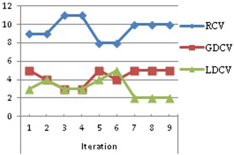
Changes in the quantities of coupling variables in Experiment 2.

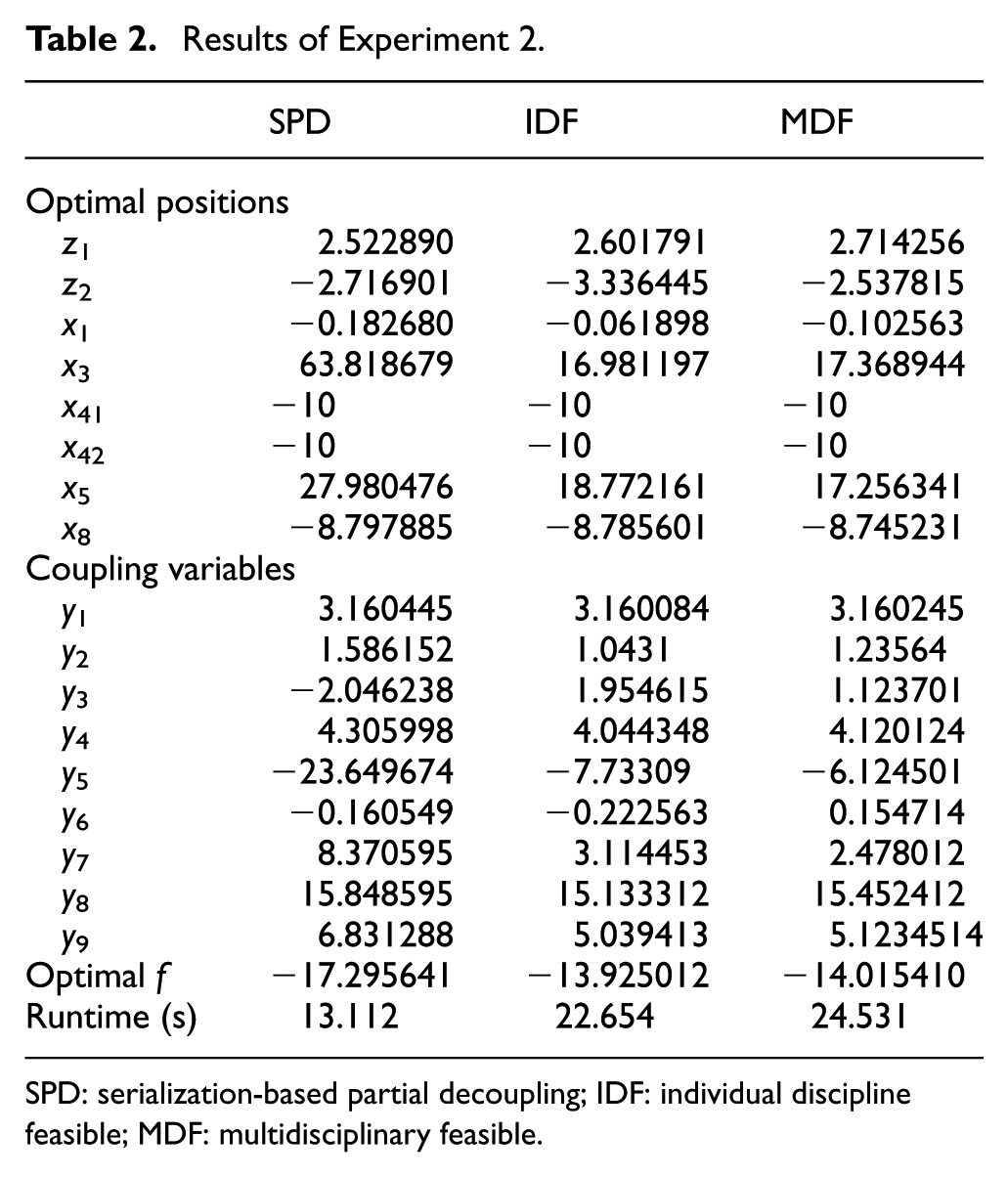
Table 2 lists the results using SPD, IDF and MDF. The optimal of the SPD method is −17.295641 whereas it is −13.925012 for IDF. Thus, the performance of the proposed SPD method is better. The time cost of SPD is 13.112 s whereas it is 22.654 s for IDF. When the SPD arrives at the optimal position, its design variables x ₃ and x ₅ have large differences from those in IDF and are much further away from the initial positions, which indicates that exploration of the search place in the SPD method is better and the objective is not restricted in the local optimal.

Table 2.

Results of Experiment 2.

	SPD	IDF	MDF
Optimal positions
z ₁	2.522890	2.601791	2.714256
z ₂	−2.716901	−3.336445	−2.537815
x ₁	−0.182680	−0.061898	−0.102563
x ₃	63.818679	16.981197	17.368944
x ₄₁	−10	−10	−10
x ₄₂	−10	−10	−10
x ₅	27.980476	18.772161	17.256341
x ₈	−8.797885	−8.785601	−8.745231
Coupling variables
y ₁	3.160445	3.160084	3.160245
y ₂	1.586152	1.0431	1.23564
y ₃	−2.046238	1.954615	1.123701
y ₄	4.305998	4.044348	4.120124
y ₅	−23.649674	−7.73309	−6.124501
y ₆	−0.160549	−0.222563	0.154714
y ₇	8.370595	3.114453	2.478012
y ₈	15.848595	15.133312	15.452412
y ₉	6.831288	5.039413	5.1234514
Optimal f	−17.295641	−13.925012	−14.015410
Runtime (s)	13.112	22.654	24.531

SPD: serialization-based partial decoupling; IDF: individual discipline feasible; MDF: multidisciplinary feasible.

This indicates that IDF is not quite suitable for highly coupled systems since a large number of constraints are added for it. MDF gets some similar results. However, when this problem is solved using SPD, the system is clustered into some subsystems, and thus, the constraints added to the global optimizer are decreased to a great extent.

Problem with multiple couplings in an engineering case

A real engineering example²⁸ involving complex coupling relationships is studied in Experiment 3. In particular, multiple couplings exist between two of the disciplines involved in this example. In this case, a combination of two simple multidisciplinary problems in MODEL of Bullalio University is adopted.²⁹ As shown in Figure 9, it is composed of the combustion of propane problem and the Golinski’s speed reducer problem. The combustion of propane problem contains three disciplines, 11 design variables, 11 coupling variables and two fixed parameters, whereas another problem contains two disciplines, seven design variables, four coupling variables and seven fixed parameters. A coupling variable y ₁₂ is constructed to combine the two problems.

Figure 9.

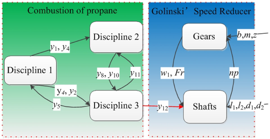
Coupling relationships of the problem solved in Experiment 3.

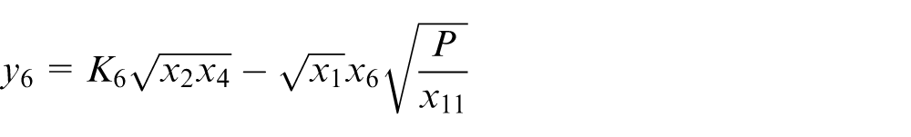
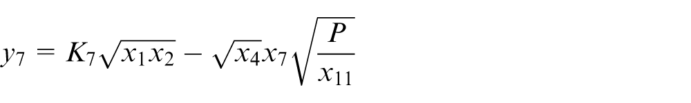
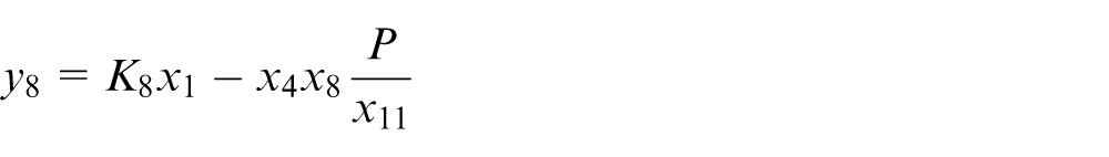
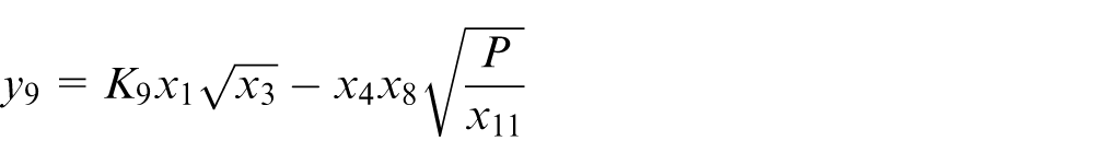
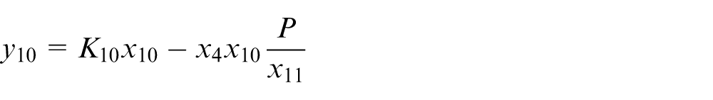
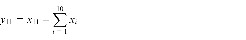
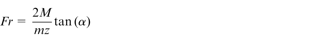
The detailed optimization model is given as follows

Minimize : f = y_{2} + y_{6} + y_{7} + y_{9} + W

(7)

Design variables: from x ₁ to x ₁₁, b, m, z, l ₁, l ₂, d ₁, d ₂

Parameters: p, R, P, r, Kg, Pd, q, Kg ₁, Kg ₂

Coupling relationships

y_{1} = x_{1} + x_{4} - 3

y_{2} = 2 x_{1} + x_{2} + x_{4} + x_{7} + x_{8} + x_{9} + 2 x_{10} - R

y_{3} = 2 x_{2} + 2 x_{5} + x_{6} + x_{7} - 8

y_{4} = 2 x_{3} + x_{9} - 4 R

y_{5} = K_{5} x_{2} x_{5} x_{4} - x_{1} x_{5}

y_{6} = K_{6} \sqrt{x_{2} x_{4}} - \sqrt{x_{1}} x_{6} \sqrt{\frac{P}{x_{11}}}

y_{7} = K_{7} \sqrt{x_{1} x_{2}} - \sqrt{x_{4}} x_{7} \sqrt{\frac{P}{x_{11}}}

y_{8} = K_{8} x_{1} - x_{4} x_{8} \frac{P}{x_{11}}

y_{9} = K_{9} x_{1} \sqrt{x_{3}} - x_{4} x_{8} \sqrt{\frac{P}{x_{11}}}

y_{10} = K_{10} x_{10} - x_{4} x_{10} \frac{P}{x_{11}}

y_{11} = x_{11} - \sum_{i = 1}^{10} x_{i}

\begin{matrix} w_{1} = [(d_{st}^{2} - d_{w}^{2}) \frac{π b}{4} + (d_{w}^{2} - d_{p}^{2}) \frac{π b}{12} + (d_{p}^{2} - d^{2}) \frac{π (2 d)}{4}] \\ * density \end{matrix}

Fr = \frac{2 M}{mz} \tan (α)

n_{p} = \frac{60 w_{1}}{2 π} rm y_{12}

In this engineering case, the quantities of RCV, GDCV and LDCV are shown in Figure 10. It can be seen from the figure that the quantity of RCV takes the majority of the total quantity. This indicates that most coupling variables are reserved. The quantities of GDCV and LDCV are 1 and 2, respectively, meaning that the global optimizer is not required to take much extra effort to explore the search space. Meanwhile, the scale of the local optimizer is not large and can be solved with a high efficiency. This experiment of the engineering case demonstrates that the coupling variables can be decoupled in a satisfactory way using the proposed architecture.

Figure 10.

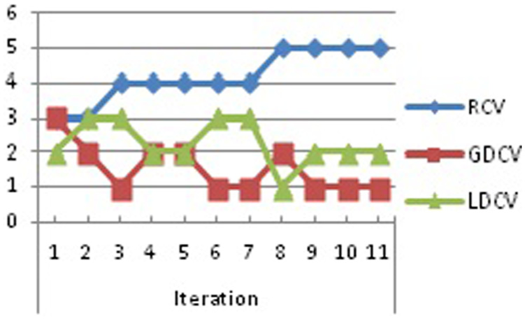
Changes in quantities of coupling variables in Experiment 3.

Table 3 lists the results obtained by solving the engineering problem in Experiment 3 using the SPD, IDF and MDF methods. The performances’ comparison helps draw a very similar conclusion to the one obtained in the previous experiment. Specifically, the MDF architecture is suitable for large-scale optimization model without complicated coupling relationships since the complete interdisciplinary analysis needs to be performed for each time of iteration. It can be seen through these two cases that the proposed SPD method is both feasible and practical for the problems with multiple complex couplings between any two disciplines.

Table 3.

Results of Experiment 3.

	SPD	IDF	MDF
Coupling variables
y ₁	1.0241423	2.145101	1.891420
y ₂	2.142575	3.012784	2.014752
y ₃	1.454147	3.147852	3.2141025
y ₄	2.478235	4.147520	9.124014
y ₅	−1.145741	−0.145368	−0.258142
y ₆	−10.25413	−8.528412	−9.857142
y ₇	2.451368	4.254145	5.256985
y ₈	6.145865	5.254369	8.369145
y ₉	9.145268	12.235456	11.256354
y ₁₀	30.254124	26.142125	36.542114
y ₁₁	−1.254147	−1.89745	−1.896521
y ₁₂	6.354896	8.567841	9.256341
Fr	2.014123	1.254156	1.568474
Np	5.214145	6.154251	7.365840
W ₁	10.254786	15.234561	16.547369
Optimal f	13.145789	18.657459	20.145786
Runtime (s)	35.145	54.214	57.235

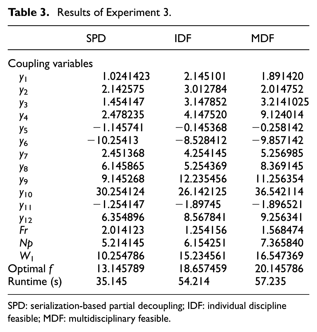
SPD: serialization-based partial decoupling; IDF: individual discipline feasible; MDF: multidisciplinary feasible.

Conclusion and future work

In this search, an SPD approach to solving MDO problems is proposed to achieve better performance in terms of complexity and efficiency. Different from the existing approaches, the SPD method has a number of features:

A three-layer framework is proposed, including the global optimizer, the subsystem solver and the local optimizer.

A clustering strategy is proposed based on sensitivity analysis, through which the multidisciplinary system is decomposed into several subsystems with reasonable and balanced scales for the subsequent analysis.

A serialization strategy is proposed for tacking the coupling relationships in a subsystem based on the directed graph theory. The main advantage of this strategy is that the solver for a subsystem can execute numerical analysis for a specific discipline with high efficiency while many coupling variables are reserved.

A local optimization process is proposed for the internal decoupled issues within a subsystem. The internal decoupled issues can be properly solved by dynamically constructing a local optimization model with a very high running speed.

In this work, some unsatisfactory issues have also been found. First, it needs the derivative information, which inevitably affects the overall performance. Additionally, the clustering operation and the serialization process should be further improved for the MDO systems involving many disciplines. Future work will be focused on exploring the combination of serialization and suspension to attain better solutions.

Footnotes

Declaration of conflicting interests

The author(s) declared no potential conflicts of interest with respect to the research, authorship and/or publication of this article.

Funding

The author(s) disclosed receipt of the following financial support for the research, authorship, and/or publication of this article: The authors appreciate the financial supports from Key Project of the Research Program of China (2013BAC16B02), NSF of China (61173126 and 61572427) and Key Project of Science and Technology of Zhejiang Province (2014C01052).

References

Joaquim

RRA

Andrew

. Multidisciplinary design optimization: a survey of architectures. AIAA J 2013; 51(9): 2049–2075.

Huang

. Development of multi-objective concurrent subspace optimization and visualization methods for multidisciplinary design. PhD Thesis, Department of Mechanical and Aerospace Engineering, State University of New York at Buffalo, Buffalo, NY, 2003.

Mastroddi

Gemma

. Analysis of Pareto frontiers for multidisciplinary design optimization of aircraft. Aerosp Sci Technol 2013; 28(1): 40–55.

Chebbah

Naceur

Hecini

. Rapid coupling optimization method for a tube hydroforming process. Proc IMechE, Part B: J Engineering Manufacture 2010; 224(2): 245–256.

Lin

Liu

Tang

et al . The coupling relationship among bottleneck shifting factors in job shop. Proc IMechE, Part B: J Engineering Manufacture 2013; 227(9): 1373–1381.

Zhang

Chen

. Thermal–mechanical coupling model-based dynamical properties analysis of a motorized spindle system. Proc IMechE, Part B: J Engineering Manufacture. Epub ahead of print 10 December 2014. DOI: 10.1177/0954405414558736.

Sobieszezanski-Sobieski

Leonard

Sirkett

. Engineering a new wrist joint replacement prosthesis—a multidisciplinary approach. Proc IMechE, Part B: J Engineering Manufacture 2002; 216: 1297–1302.

Weck

Agte

Sobieszezanski-Sobieski

. State-of-the-art and future trends in multidisciplinary design optimization. In: Proceedings of the 48th AIAA/ASME/ASCE/AHS/ACS structures, structural dynamics, and materials conference, Honolulu, HI, 23–26 April 2007, paper no. AIAA-2007-1905. Reston, VA: AIAA.

Myers

Montogomery

. Response surface methodology: process and product optimization using designed experiments. New York: Wiley, 1995.

10.

Braun

Kroo

. Development and application of the collaborative optimization architecture in a multidisciplinary design environment. Multidisciplinary Design Optimization: State of the Art 1995; 5: 98–116.

11.

Zadeh

Toropov

Wood

. Metamodel-based collaborative optimization framework. Struct Multidiscip O 2009; 38(2): 103–115.

12.

Sobieszezanski-Sobieski

Chopra

. Multidisciplinary optimization of aeronautical system. J Aircraft 1990; 12: 977–978.

13.

Michalek

. Diagonal quadratic approximation for parallelization of analytical target cascading. J Mech Des: T ASME 2008; 130(5): 051402-1–051402-11.

14.

Tappeta

Renaud

. Multi-objective collaborative optimization. J Mech Des: T ASME 1997; 119(3): 403–411.

15.

Simpson

Mistree

Korte

. Kriging models for global approximation in simulation-based multidisciplinary design optimization. AIAA J 2001; 39(12): 2233–2241.

16.

Han

. Multidisciplinary design optimization approaches and technique research for complex engineering systems. Beijing, China: Beijing University of Aeronautics and Astronautics, 2004.

17.

Yao

Chen

Luo

. Review of uncertainty-based multidisciplinary design optimization methods for aerospace vehicles. Prog Aerosp Sci 2011; 47(6): 450–479.

18.

Wang

. A CAD/CAE integrated framework for structural design optimization using sequential approximation optimization. Adv Eng Softw 2014; 76: 56–68.

19.

Patnaik

Hopkins

. General-purpose optimization method for multidisciplinary design applications. Adv Eng Softw 2000; 31: 57–63.

20.

Sobieszezanski-Sobieski

. Sensitivity of complex internally coupled systems. AIAA J 1990; 28(1): 153–160.

21.

Sell

Batill

Renaud

. Response surface based concurrent subspace optimization for multidisciplinary system design. In: Proceedings of the 34th aerospace sciences meeting and exhibit, Reno, NV, 15–18 January 1996, paper no. AIAA 96-0714. Reston, VA: AIAA.

22.

Sobieszczanski-Sobieski

Agte

Sandusky

. Bi-level integrated system synthesis (BLISS). NASA/TM-1998-208715, http://ntrs.nasa.gov/archive/nasa/casi.ntrs.nasa.gov/19980234657.pdf

23.

Qiu

Feng

Dong

. Approaches for analyzing the optimization results based on the sensitivity information. J Zhejiang Univ: Sc B 2000; 34(6): 603–607.

24.

Irene

Ramon

Charles

. Quadratic programming feature selection. J Mach Learn Res 2010; 11: 1491–1516.

25.

Justin

Kenneth

. Standard platform for benchmarking multidisciplinary design analysis and optimization architectures. AIAA J 2013; 51(10): 2380–2394.

26.

Chan

. Evaluation of two concurrent design approaches in multidisciplinary design optimization. NRC report LM-A-077, January 2001.

27.

Hulme

Bloebaum

. Development of CASCADE—a multidisciplinary design test simulator. In: Proceedings of the 6th symposium on multidisciplinary analysis and optimization, Bellevue, WA, 4–6 September 1996. Reston, VA: AIAA.

28.

Roy

Hinduja

Teti

. Recent advances in engineering design optimisation: challenges and future trends. CIRP Ann: Manuf Techn 2008; 57(2): 697–715.

29.

Parashar

. Decision support tool for multidisciplinary design optimization using multi-domain decomposition. In: 46th AIAA/ASME/ASCE/AHS/ASC structures, structural dynamics & materials conference, Austin, TX, April 2005.

A serialization-based partial decoupling approach for multidisciplinary design optimization of complex systems

Abstract

Keywords

Introduction

Overview of the SPD method

SPD flowchart

SPD framework

Clustering analysis based on sensitivity

Sensitivity analysis

Subsystem clustering based on sensitivity

Decoupling of a subsystem

Connection path between disciplines

SPD process in a subsystem

General process of partial decoupling based on serialization

Formal demonstration of loop removal

Illustration of the whole SPD process

Serializable solving in a subsystem

Local optimization in a subsystem

Computational experiments

Partial decoupling of a single subsystem

Serializable decoupling of multidisciplinary problems

Problem with multiple couplings in an engineering case

Conclusion and future work

Footnotes

Declaration of conflicting interests

Funding

References