Automatic experimental modal analysis of milling machine tool spindles

Abstract

Dynamic compliance of machine tool spindle is a necessary input for stability limit prediction. It can be determined by a single input–single output modal analysis, so called tap test. Despite methodology of modal analysis is well known for many years and there are several commercially available software packages supporting it, executing the experiments and evaluation of the results require both knowledge and skill. Therefore, there is a need for automation of all stages of data acquisition and signal processing to make this method applied in industry. This article presents the methodology, algorithms and software which execute all operations and analysis automatically; thus, they can be done directly on the factory floor without the involvement of highly qualified personnel. It enables completing of the tap test and obtaining proper results by an operator who do not have any knowledge on modal analysis. This article presents examples of the software application in factory floor conditions.

Introduction

Self-excited vibrations (chatter) not only limits productivity of machining processes but also causes poor surface finish and early wear/breakage of cutting tools. ¹ Thus, prediction of the chatter onset is critical for the realization of productive machining. Basic input for the calculation of the stability limit is frequency response function (FRF) of the machine tool structure obtained from single input–single output (SISO) modal analysis.^1,2 During so called tap test, the machine tool spindle or a tool held in it is excited with a modal hammer with built-in force transducer. The response of the machine tool structure can be measured with an accelerometer. The FRF is then determined by combining the Fourier spectrum of both the impact force measurement and the accelerometer measurement. Resultant dynamic compliance or FRF of the spindle allows for determination of specific combination of machining parameters that results in the maximum chatter-free material removal rate.

Modal analysis allows for computing of modal parameters (frequency, damping, stiffness and mass) of vibrating system. During the tap test, the energy of the impulse excitement is distributed continuously in the frequency domain. A force impulse excites all frequencies within its useful frequency range, which is inversely proportional to the duration of the impulse. ³ Modal hammer tips of different hardness allow for a different impulse time excitement. ⁴ In the SISO modal analysis, vibrations of a tool or specially prepared shank clamped in the spindle are induced by the hit of a modal hammer and measured by an accelerometer fixed on the other side of the tool.^{5 –7} Assuming that the system is linear, time-invariant, it can be represented as the linear superposition of a number of single-degree-of-freedom (1DOF) characteristics. FRF G(f) of 1DOF system is equal to the inverse of the dynamic stiffness of the system in the frequency domain ⁸

$$G\left(f\right)=\frac{1}{-m{\left(2\pi f\right)}^2+\mathrm{jc}\left(2\pi f\right)+k}$$

(1)

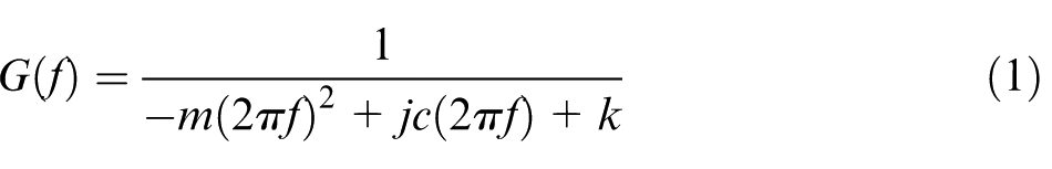
where m is the mass (kg), c is the damping coefficient (Ns/m) and k is the stiffness (N/mm).

A characteristic point of the system dynamic compliance is its minimum real part which determines the minimal stable axial depth on the stability lobe diagram (see Figure 1). Therefore, Re(G)_min is an important indicator of machine resistance to self-excited vibrations and can be used as the indicator of machine tool spindle condition. Systematic measurement of FRF and Re(G)_min provides a means of monitoring of the spindle condition degradation and for planning of preventive service. Therefore, it should be done directly on the factory floor without the involvement of highly qualified personnel.

Figure 1.

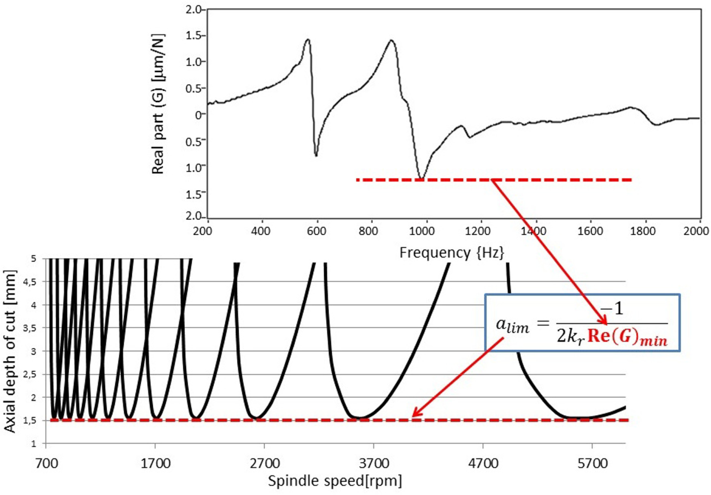
Dependence of stability lobe diagram on minimum real part of dynamic compliance based on Altintas and Weck. ⁹

Modal parameters of such system—mass, damping and stiffness—can be calculated from FRF for each modal mode separately using characteristic features of the real and imaginary parts of FRF^4,5,10 (see Figure 2). The resonance frequency f₀ is being identified directly as the local minimum (valley) in the imaginary part of the FRF—Im(G). Damping ratio can be determined by the following formula

$$d=\frac{(f_2-f_1)}{\left(2f_0\right)}$$

(2)

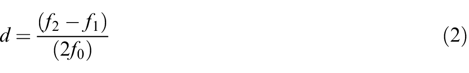
where f₁ and f₂ are the nearest maximum and minimum of Re(G) surrounding f₀, respectively. Stiffness coefficient can be found from a minimum value of Im(G)

$$k=\frac{-1}{\left(2d\mathrm{Im}{(G)}_{\min }\right)}$$

(3)

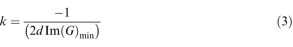
and modal mass is equal to

$$m=\frac{k}{{\left(2\pi f_0\right)}^2}$$

(4)

Figure 2.

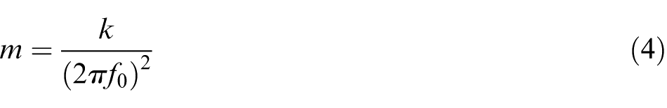
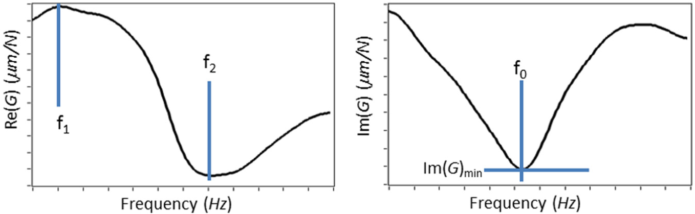
FRF characteristic features of single mode.

Finally, modal damping can be calculated as

$$c=2d\sqrt{\mathrm{km}}$$

(5)

Presented methodology is well known and seems to be quite easy. Unfortunately, it is not in factory floor practice.

Difficulties in the tap test signal processing and FRF interpretation

During the tap test, the operator implements several hits of the modal hammer into the special shank clamped in the spindle. Next subsequent single excitement and response signals must be identified and extracted from the entire acquired force and acceleration signals. The segmented signals covering single hits have to be evaluated for their correctness—proper signal amplitude, absence of saturation of the signal (overload of preamplifier) or double hits. Wrong signals (force and vibration) must be eliminated, because using them in the analysis makes results unreliable (see Figure 3).

Figure 3.

Wrong excitations and responses.

Double hits as well as leakage and an overload of accelerometer preamplifier can be seen in the signals. A selection of short fragments of measured signals containing the actual exciting force and object acceleration signals is an important and time-consuming stage of experimental modal analysis. Browsing the entire signal, assessing every force and response signal and rejecting non-proper ones require lots of time, experience and attention from the operator.

After collecting correct signals, their spectra are calculated, which allow for computing of the average FRF. Next troublesome step is identification of frequency ranges corresponding to the singular modes. It is based on selection of the frequency range of the individual mode in real and imaginary part of the FRF. Synchronized observation of the two plots increases accuracy of such selection (Figure 4).

Figure 4.

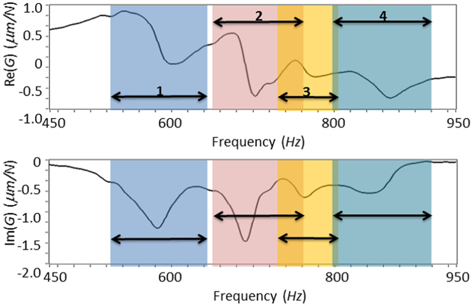
Frequency ranges.

When the frequency range corresponding to a particular mode is identified, modal parameters can be determined from characteristic features of real and imaginary parts of the FRF according to formulas (2)–(5).^11,12

Then, analyzing obtained FRF, selection of the frequency ranges corresponding to the single modes and determination of FRF features (f₀, f₁, f₂) are another difficult and time-consuming procedures which require experience and knowledge about modal analysis.^13,14 In case of distorted Re(G) and Im(G), or modes of close frequencies, proper selection of these frequency ranges is demanding even for experienced operator.^15,16

There is a lot of commercial software focused on an area of modal analysis; however, there is a lack of software which is helpful in SISO modal analysis and modal parameters. Execution of modal analysis is difficult even using professional, excellent commercial software like CutPro ¹⁰ which results in withdrawal from using it. Therefore, broader implementation of modal analysis in the industry necessitates automation of the entire process of signal acquisition, segmentation, evaluation, mode frequency range identification and modal parameter calculation.

Automatic modal analysis

The motivation of the project ¹⁷ was inspired by requests of aerospace industry partners, who need modal analysis, but have no enough experience, highly qualified personnel to use CutPro ¹⁰ in everyday practice. The developed software^{15 –17} gathers expert experience in manual modal analysis, signal processing and converts it into computer algorithms.

Signal segmentation

An automatic signal segmentation is based on the detection of the beginning of a single hit. It is recognized in the force signal as exceeding of a threshold, which is five times higher than the maximum value during the first 5 ms of entire signal (see Figure 5). Then, the segment of 50 ms of the signal is extracted, beginning from the 5 ms preceding the threshold crossing. 50 ms is far longer time than needed for decreasing of the damped vibration signal below a noise level.

Figure 5.

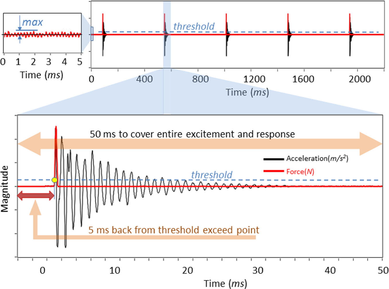
Hits and responses extraction method.

Selection of correct signals

The extracted excitement and response signals must be examined to identify whether they are correct, meaning meet the following criteria

• Maximum of the excitement force is higher than 10 N;

• Absence of signal saturation indicating overload of hammer and/or accelerometer preamplifiers;

• Absence of double hit, the hammer bounce—occurrence of the second maximum of the force signal within 50 ms window.

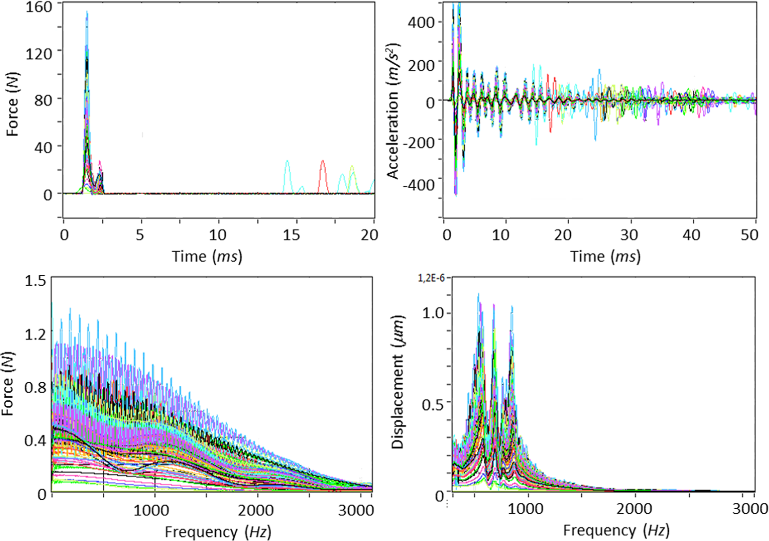
Out of all correct signals, five with highest maximum force are taken for further analysis. Figure 6 presents example of time domain signals extracted from entire signal using presented criteria and their spectra.

Figure 6.

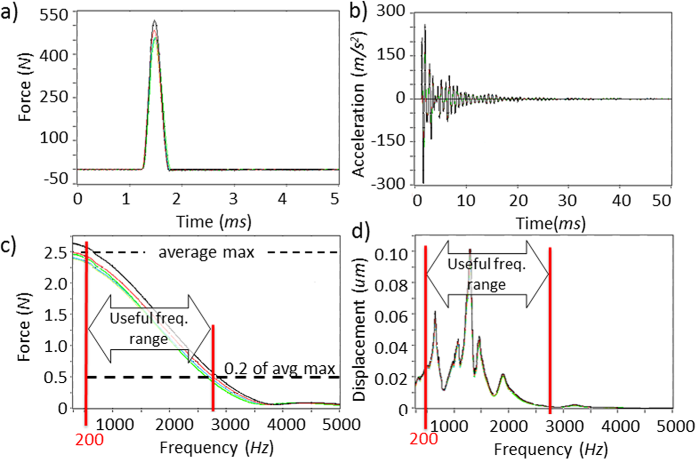
(a) Extracted time domain signals of hammer excitation, (b) system responses and (c, d) their spectra.

Automatic mode detection

As spectrum of the excitation signal descends with the frequency, the FRF becomes less reliable. Thus, frequency range is assumed to be useful when average excitation spectrum is higher than 20% from its maximum value. ⁷ On the other hand, because the response of the structure is measured using accelerometer, the signal needs to be integrated twice in frequency domain, in order to get the displacement. This results in extremely high, also unreliable signal values for the lowest frequencies. Therefore, in the example presented in Figure 6, the useful frequency range was limited from the left side—to 200 Hz. Of course, this lower limit can be changed if more massive structures of lower natural frequencies are to be analyzed.

In the next step, complex FRFs are computed for every extracted excitation and response signals, and obtained results are averaged. Then, the coherence function is calculated and used for assessment of distortion, lack of correlation or non-linearity. The function value is 1 for linear system with no distortion of input and output. ⁹ It can have values between 0 and 1, and values closer to 0 indicate distortion, lack of correlation or non-linearities.

Automatic mode detection begins with searching of local minima in Im(G) FRF (see point 1 in Figure 7). Every minimum indicates potential resonance frequency f₀; however, there are usually hundreds of them, mostly accidental, irrelevant. The following procedure is applied for identification of actual system modes. First, the nearest Im(G) local maximum on the left (point 2 in Figure 7) and on the right (point 3 in Figure 7) from the detected local minimum is detected. The frequencies corresponding to these detected local maxima indicate the frequency range for a single mode. Then, the following criteria are used for the validation of the mode relevance: coherence function value at modal frequency f₀ is higher than 0.6 and modal frequency f₀ is within the useful range. Examples of automatically detected modes and their frequency ranges are shown in Figure 8. The presented method enables to detect also closely located modes. It could be difficult even for experienced users applying manual identification of the modes.

Figure 7.

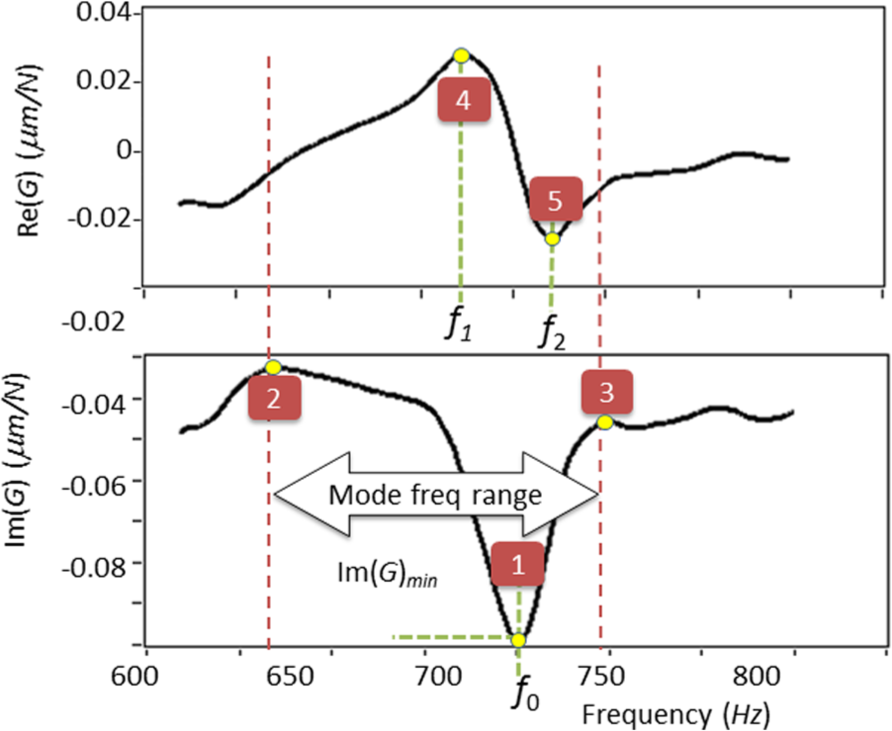
Automatic mode detection method.

Figure 8.

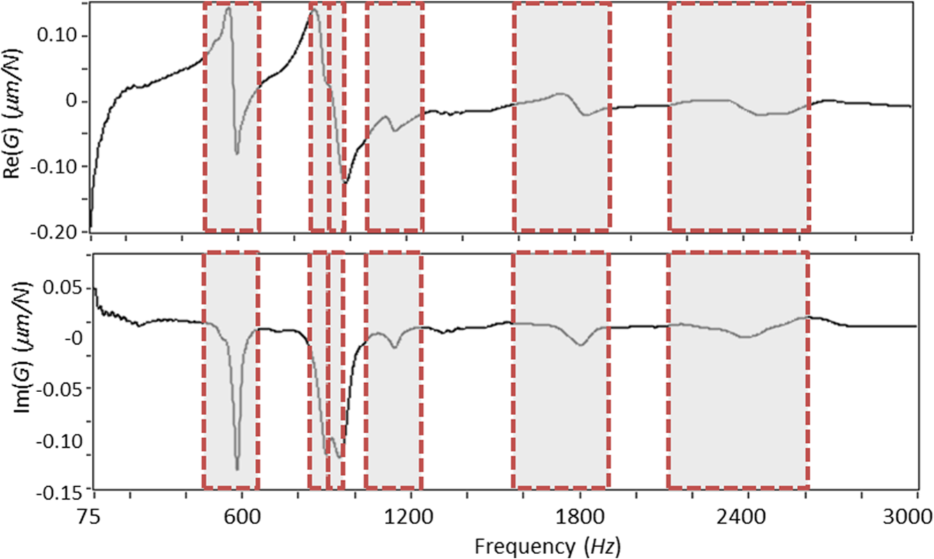
Recognized frequency ranges.

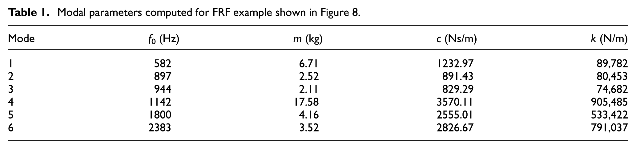
For the modes considered relevant, nearest maximum and minimum values of Re(G), the corresponding frequencies f₁ and f₂ (points 4 and 5 in Figure 7) are identified within each mode frequency range. Thus, for every mode values of f₀, f₁, f₂, Im(G)_min are obtained and used for calculation of modal parameters according to formulas (2)–(5). Modal parameters computed for frequency ranges from the example shown in Figure 8 are presented in Table 1.

Table 1.

Modal parameters computed for FRF example shown in Figure 8.

Mode	f 0 (Hz)	m (kg)	c (Ns/m)	k (N/m)
1	582	6.71	1232.97	89,782
2	897	2.52	891.43	80,453
3	944	2.11	829.29	74,682
4	1142	17.58	3570.11	905,485
5	1800	4.16	2555.01	533,422
6	2383	3.52	2826.67	791,037

Modal parameters applied in equation (1) give the FRF model, shown in Figure 9. As can be seen here, when system modes are widely separated from each other, FRF model is correct (e.g. for 1st, 5th and 8th modes). However, if the system modes are located closely (especially 2nd and 3rd modes in Figure 9), the modes influence each other which results in overestimation of the system compliance, and dramatically reduces the correlation between experimental and estimated FRFs.

Figure 9.

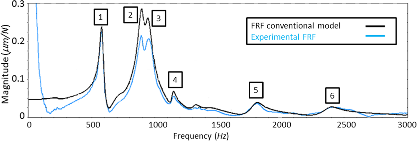
Automatic modal analysis result—modeled versus experimental FRF.

Automatic optimization of the FRF model

A difference between the model and experimental function can be noted in Figure 9 for frequency range corresponding to 2nd and 3rd modes. Let us consider only these two modes and calculate 2DOF FRF model of the system. By substituting modal parameters from 2nd and 3rd rows of Table 1 into the transfer function equation (1), two single plots, each representing the single mode, are obtained (see Figure 10). The 2DOF characteristic is then found by superposition of single modes. Superposition of modes closely located to each other results in overestimation of modal damping and poor correlation between experimental and estimated characteristics.

Figure 10.

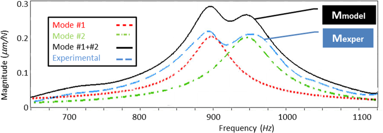
Characteristics of 2DOF system obtained by mode superposition.

In order to increase correlation between experimental and estimated FRFs, the methodology of modal damping optimization was developed. It is based on iterative changes of single-mode damping by comparing the resultant entire model correlation with the experimental FRF.

Automatic optimization of the model is implemented in three successive stages. Each of the stages aims to damping adjustments minimizing the difference between the magnitude of the model and the experimental FRF at modal frequency seen in Figure 10. The magnitude of modeled FRF (M_model) at the modal frequency of individual mode is compared with the magnitude of the experimental FRF (M_exper). If the absolute value of the difference X = (M_model − M_exper) is higher than 0.005 µm/N, and if the FRF magnitude is too small, the damping of the considered mode is increased by 10%. When the magnitude is too high, the damping is reduced by 10%. Then, the entire model is recalculated. When the difference X is lower than 0.005 µm/N, the allowed difference is reduced to 0.002 µm/N and the procedure is repeated. Then, optimization of next mode is started. Results of application of this procedure are presented in Figure 11.

Figure 11.

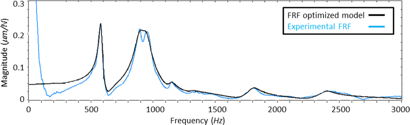
Comparison of optimized with the experimental FRF.

Automatic adjustment of modal damping allows for increasing the correlation between experimental and estimated FRFs being still simple mathematical method.

Automatic Single-Input-Single-Output Modal Analysis software

Methods and algorithms described in the previous section were applied in Automatic Single-Input-Single-Output Modal Analysis (ASISOMA) software programmed in the NI LabVIEW environment. In industrial default mode, the user is guided through stages of experiments and analysis until getting the results of modal analysis, which are modal characteristics and minimum of real FRF part—Re(G)_min as dynamic compliance indicator. The scientific mode can be used in industry, but it is dedicated for educational purposes. Manual mode selection can be used in the scientific mode of the program. It makes it easy to understand how 1DOF modal analysis works and how characteristic features of the complex FRF look like. In a scientific mode with the manual mode selection, user is responsible for rejecting improper modes. Failure of complying with specified criteria used in automatic mode program computes modal parameters of every frequency range regardless of its physical meaning. The program calculates the complex FRF model and presents it in several forms: amplitude–frequency characteristic, phase–frequency characteristic and also Re(G) and Im(G) on the hodograph as amplitude–phase–frequency characteristic (see Figure 12).

Figure 12.

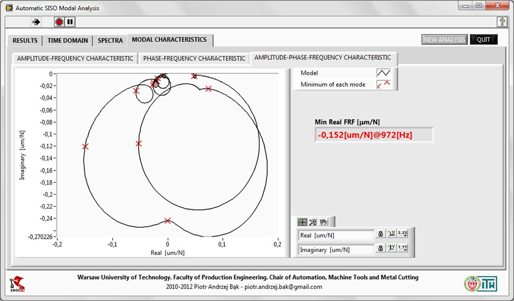
Examples of ASISOMA program front panel working in the scientific mode.

Example of ASISOMA front panels in this mode is presented in Figure 13. The picture presents dynamic compliance with its modal parameters.

Figure 13.

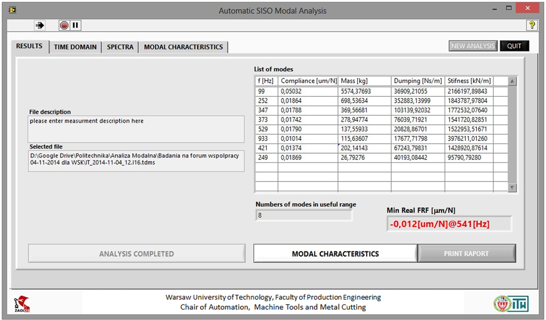
Examples of ASISOMA program front panel working in the industrial mode.

Experimental setup

Measurement setup for 1D SISO modal analysis is simple and easy to use in factory floor conditions. It consists of a modal hammer (here, it is Brüel & Kjær 8206-03), accelerometer (here, B&K 4514-001), conditioning amplifier (here, B&K NEXUS 2693), DAQ card (here, NI USB-6259 BNC) and PC with LabVIEW 2010 environment (Figure 14).

Figure 14.

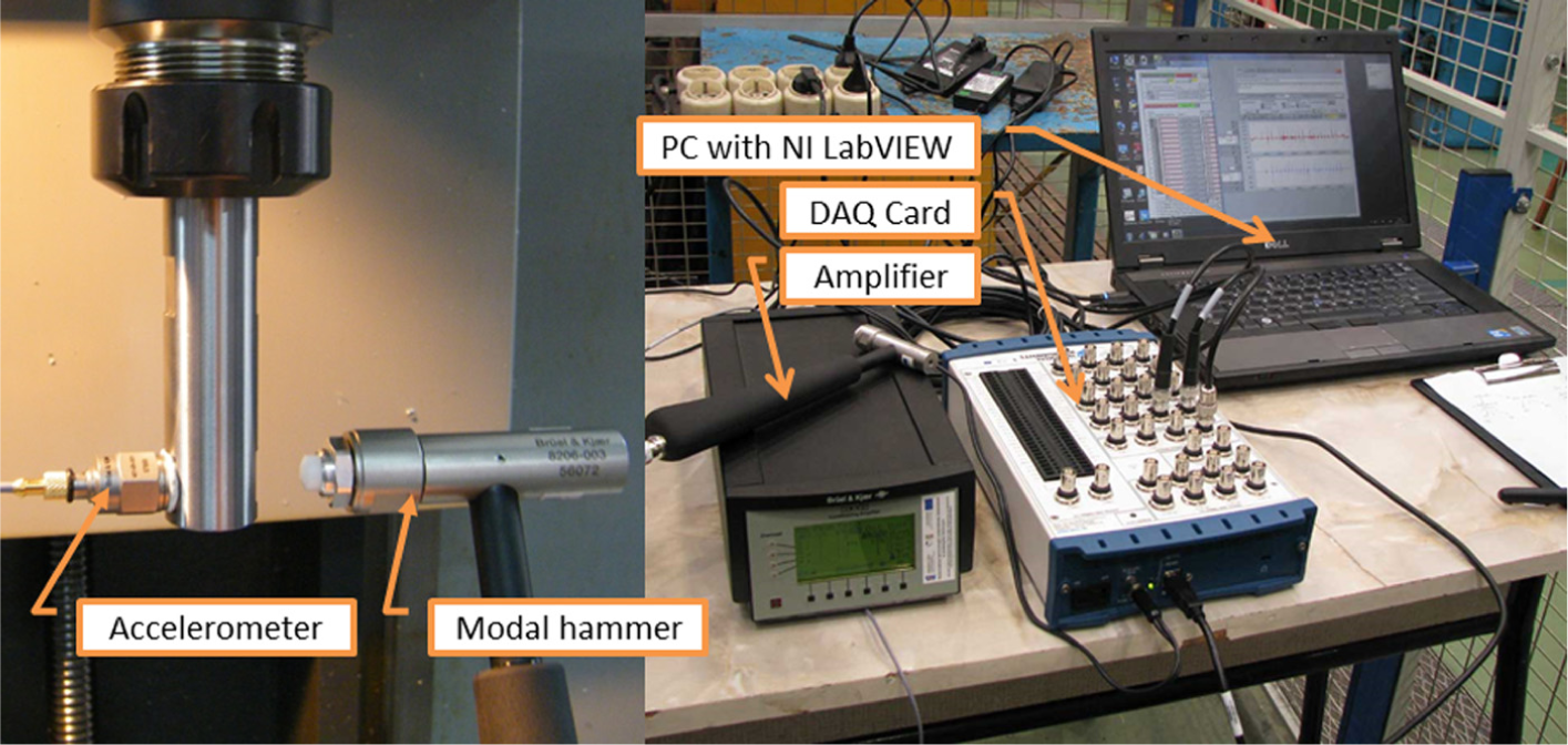
Measurement setup.

Industry application

Described methodology was applied in the aerospace industry facility in the Aviation Valley in Poland. ¹⁷ The objective of the test was determination of dynamic condition of 12 identical computer numerical control (CNC) machining centers (two lines, six machines in each line) DMU 70 eVo Linear. The developed software automatically creates reports with obtained results. Examples of parts of it are presented in Figure 15.

Figure 15.

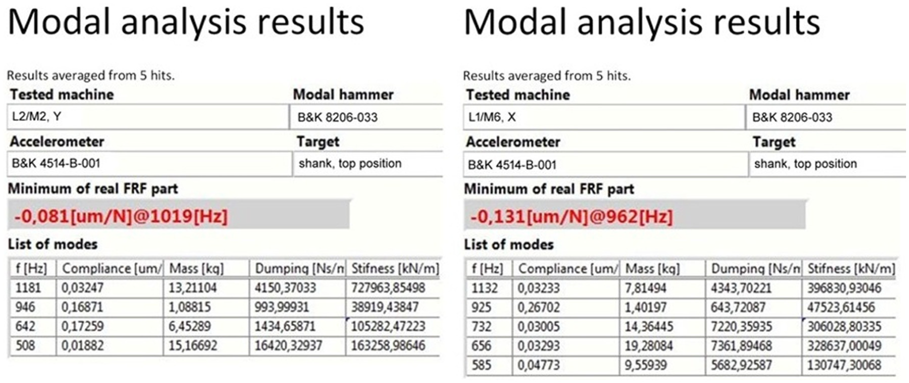
Fragments of automatically generated report on the SISO modal analysis.

The most indicative of the chatter resistance is the minimum of real part of FRF. These values for all 12 tested machines are presented in Figure 16. The average values are marked by a dashed line. Values much lower than average were considered as safe (green field), and values much higher than average were considered as indication for maintenance. One machine—the third in the first line—appeared to be in the worst condition. Actually, it was already withdrawn from production, waiting for maintenance. The best results on both axes were achieved by machine two in the second line.

Figure 16.

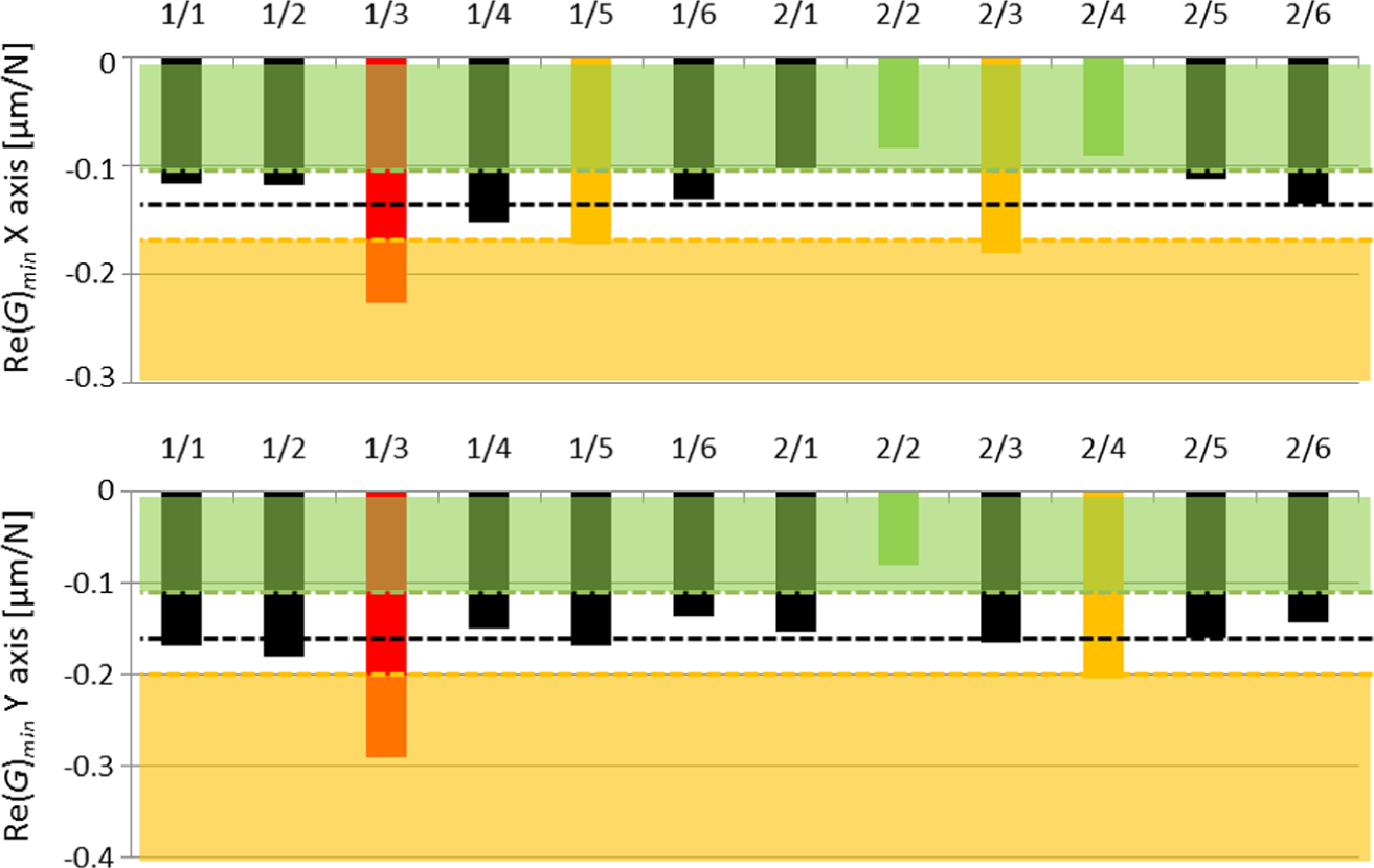
Dynamic compliance of tested high-speed spindles.

Simultaneously, the speed spindle error motions were tested according to ANSI/ASME Standard B5.54-1992 ¹⁸ with our own software. ¹⁹ Obtained results (example shown in Figure 17) confirm those presented by the automatic modal analysis. Machine 2/2 has the lowest measured dynamic compliance and total radial error movement 5.6 µm. On the other hand, machine 2/4, which is on the Y axis exceeded warning level, has total radial error movement more than twice higher—12.1 µm.

Figure 17.

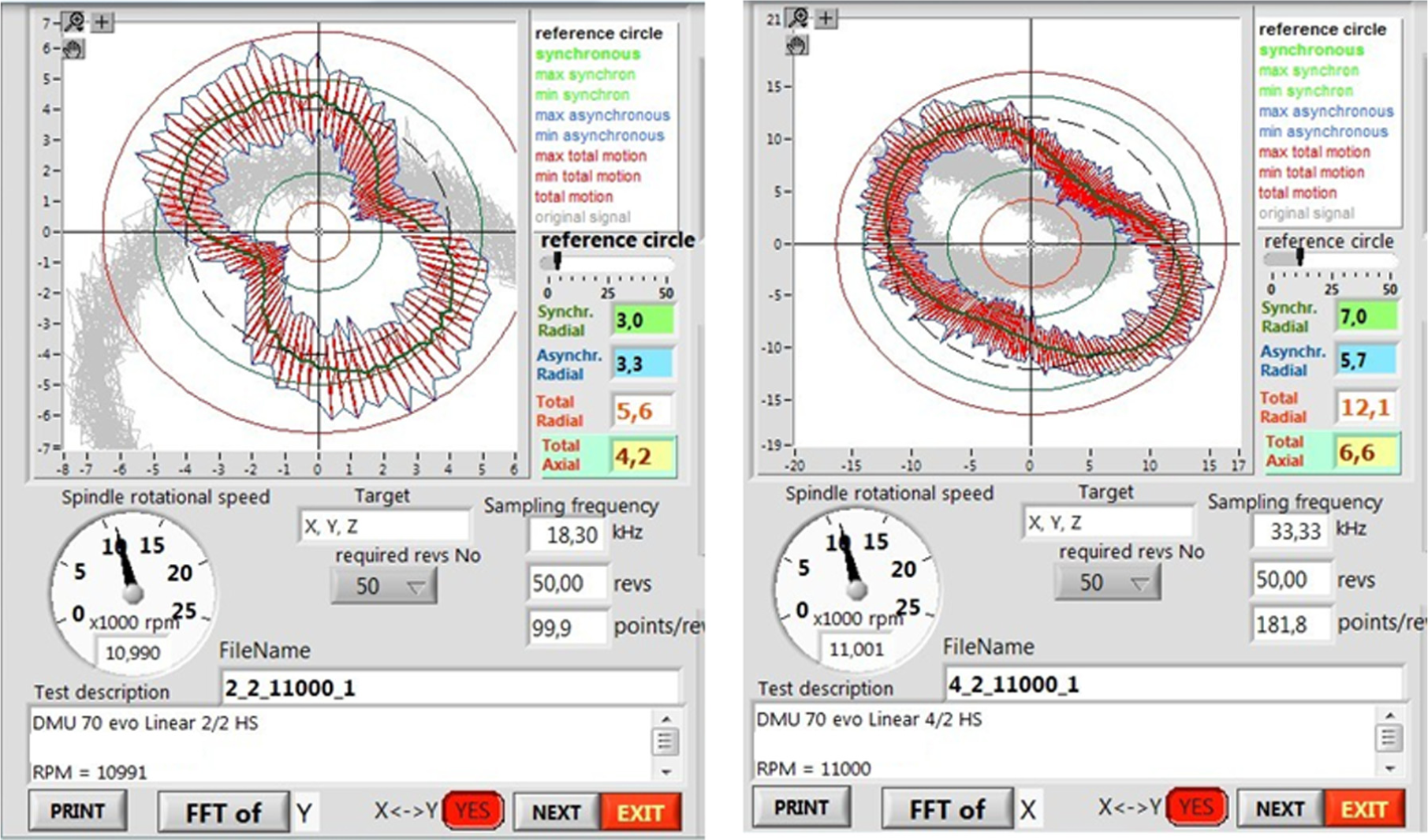
Example of the speed spindle error motion testing.

Conclusion

Conventional experimental modal analysis requires both knowledge and skill for evaluation of registered signals, selection of the proper hits and selection of the frequency ranges corresponding to the single modes. All this necessary knowledge and skills were converted into algorithms by innovative application of modal analysis formulas and signal processing methods. Using the software developed on the base of these algorithms, all necessary operations and analysis are automatized; thus, they can be executed directly on the factory floor without the engagement of highly qualified personnel.

The experimental test performed in factory floor conditions confirms the usability of developed automatic modal analysis methodology and the software.

While working in the industrial mode, the program performs all necessary calculation without operator intervention. Only few hits are needed with a modal hammer while measuring acceleration to have a ready characteristic in a moment. The program automatically executes the following steps:

• Extraction of hit and responses from entire signal, with rejection of non-proper ones;

• Computation of signal spectra and FRF;

• Detection of vibration modes, rejecting irrelevant ones;

• Calculation of the complex FRF model ready to be presented in several forms: amplitude–frequency characteristic, phase–frequency characteristic and amplitude–phase–frequency characteristic (hodograph).

Created ASISOMA software not only has different interface and/or functionality than existing on the market but also creates a new added value due to full automatization of signal evaluation and processing.