
Abstract
Despite significant advances in modelling and design, mechanical systems almost inevitably fail at some point during their operative life. This can be due to a pre-existing design flaw, which is usually overcome in a revision, or more commonly due to some unexpected damage during operation. To overcome a failure during operation, a new method in designing machines or systems is proposed that creates a result, that is, resilient to both expected and unexpected failure. By shifting the focus from a detailed assessment of the underlying cause of failure to how that failure will manifest, a system becomes inherently resilient against a wide range of failure modes. The proposed process involves five steps: cause, detection, diagnosis, confirmation and correction. This is demonstrated with an application to a generic 4 bar linkage mechanism. Through this process, the system is able to return to a near perfect state even after a permanent deformation occurs in the mechanism. These results show the potential that this self-repairing design process has applications including robotics, manufacturing and other systems.
Introduction
In an era of rapid technological development, largely driven by significant advances in computational power and global collaboration, engineering systems are becoming exponentially more complex and less reliable. Although improvements in maintenance regimes and through-life services can enhance the reliability of systems, it is almost inevitable that failure will occur at some point during their operation and these failures are often due to unexpected events. 1 Providing reactive maintenance following an unexpected failure is often expensive and can be impossible to achieve quickly (if at all) in certain circumstances, for example, during space exploration. Several current design approaches exist to mitigate the risks associated with failures in operation: system redundancy can be built in; 2 controllers can be employed to cope with damaged hardware 3 and systems can be pre-programmed to cope with certain types of specific failures. 4 Although these methods are adequate for designing against anticipated failures, achieving robust performance under uncertainty is far more difficult. 5 Self-healing is a phenomenon most commonly associated with biological systems, for example, mammalian skin and its ability to repair after serious injury to a fully functional state. An alternative to this is the term ‘self-repairing’ often commonly associated with physical systems such as electronics or mechanical systems that can similarly exhibit some ability to regain a fully functional state. Self-healing can be seen as a bottom-up approach, where the components of the system heal any damage from the inside. 6 Much work conducted into self-healing technologies has focused upon the material level, such as self-healing composites.7,8 Here, passive systems provide the structure with regenerative properties in an attempt to restore its strength following a structural failure. Such passive systems offer potential for coping with small-scale structural damage; however, large deviations from the undamaged structural state may require additional input to re-align severely damaged structures in order to maintain a reasonable level of functionality (cf. broken bones in animals). For a system to repair under these circumstances, it would have to identify damage before deciding on the best course of action to correct the damage.
Much like adaptable design, 9 self-repairing systems require specific design methodologies to maximise the benefits offered to the mechanical system under consideration. Designing for self-repair is a top-down approach where the system is designed to have the ability to maintain its own function through external factors such as diagnosis and reconfiguration. Autonomous self-repairing systems for example, are able to detect and diagnose faults then either isolate the fault and replace components, or repair the damage through external actions. 6 Such characteristics provide a system that can therefore identify and correct unanticipated damage. Recent work by Koos et al. proposes an algorithm that allows machines to adapt to failure modes by learning from an internal model of themselves. They test their algorithm with application to a hexapod robot and show that it offers significant performance advantages over other robust design methodologies, such as optimised control-based methods. 1 Although the proposed algorithm can maintain certain functionalities, it does not explore the possibility of the machine repairing the physical damage. This is because in general terms, what is often desired is a system, that is, able to ‘maintain some degree of functionality after a failure has occurred’. 10 A further discussion on the taxonomy of self-healing and self-repairing systems and their differences can be found in the work by Frei et al. 6
To achieve a self-repairing system, it is clear that the system must have an element of self-awareness. Amor-Segan et al. 11 originally stated that what is desired is a system that has ‘the ability to autonomously predict or detect and diagnose failure conditions, confirm any given diagnosis, and perform appropriate corrective intervention(s)’. From this description, the ‘design for self-repairing’ process has previously been broken down into five steps: 12
Cause of fault. This is numbered as such because in an ideal ‘self-repairing’ system, the underlying cause of fault is irrelevant. Instead, the system should be designed in such a way that all underlying causes are mitigated against by focusing on how these causes might manifest;
Detection of fault. All underlying faults within a system will inevitably lead to a fundamental change in the behaviour or output (else it could be argued that a fault has not occurred);
Diagnosis. Once a fault has been detected, the system must then determine where and how that fault has occurred;
Confirmation of diagnosis. Any fault that is diagnosed will have an associated confidence level based on how certain the diagnosis is. In some cases, this will be sufficient to instigate a corrective action, in other cases, where multiple points of failure could be the culprit, it is important to confirm the diagnosis to avoid rerouting or replacing potentially unfaulty components.
Corrective action. Perhaps the most significant aspect of the self-repairing process, this will be an application specific; however, a number of possible approaches are available, which are discussed in more detail later.
It should be highlighted that closed-loop systems mirror much of the steps highlighted in above, with monitoring and diagnosis abilities used to control and optimise certain functions of a component or device, for example, in a heating, ventilation and air conditioning (HVAC) system. However, there are a number of differences to these systems and the field of self-repair.
First, self-repair looks to overcome the loss or degradation of function whereas most control systems focus upon maintaining an optimised state in response to some kind of variation, often environmental in the case of HVACs. Self-repair often goes further than feedback systems when it comes to repair with actions resulting in the removal of damaged components, for example, found in systems with many redundant parts such as electronics, or physical components such as self-repairing robotics as discussed previously. Closed-loop systems often monitor simple parameters such as environmental change, while self-repairing systems have to cope with higher levels of complexity with regard to detection and diagnosis as the source of damage is often irregular and non-deterministic. The complication of most repairing strategies being one-off solutions makes taking the correct action crucial as it is not always possible to go back after corrective action has been employed.
To demonstrate the above process, this article uses an example of a simulated 4 bar linkage mechanism. Mechanical linkages are, at a basic level, an assembly of rigid elements connected via joints to translate motion or force. Planar linkage mechanisms with revolute joints are widely used in industry either to transmit torque, motion and power, or to transform one type of motion or force to another. 13
From a theoretical point of view, 4 bar linkages have been most extensively covered in the literature due to their relative simplicity, making them an ideal case study for a proposed self-repairing design approach. A simple example of a 4-bar linkage is shown in Figure 1. It is assumed that the mechanism is designed to trace a particular pattern. The apex of the triangular coupler link will follow a particular pattern when the input link is rotated to one complete revolution. The specific pattern will depend on the geometry/length of the four links and the geometry of the triangular float link, which can be described completely by the length of l 1 and the two other tracer edge lengths (t 1 and t 2).
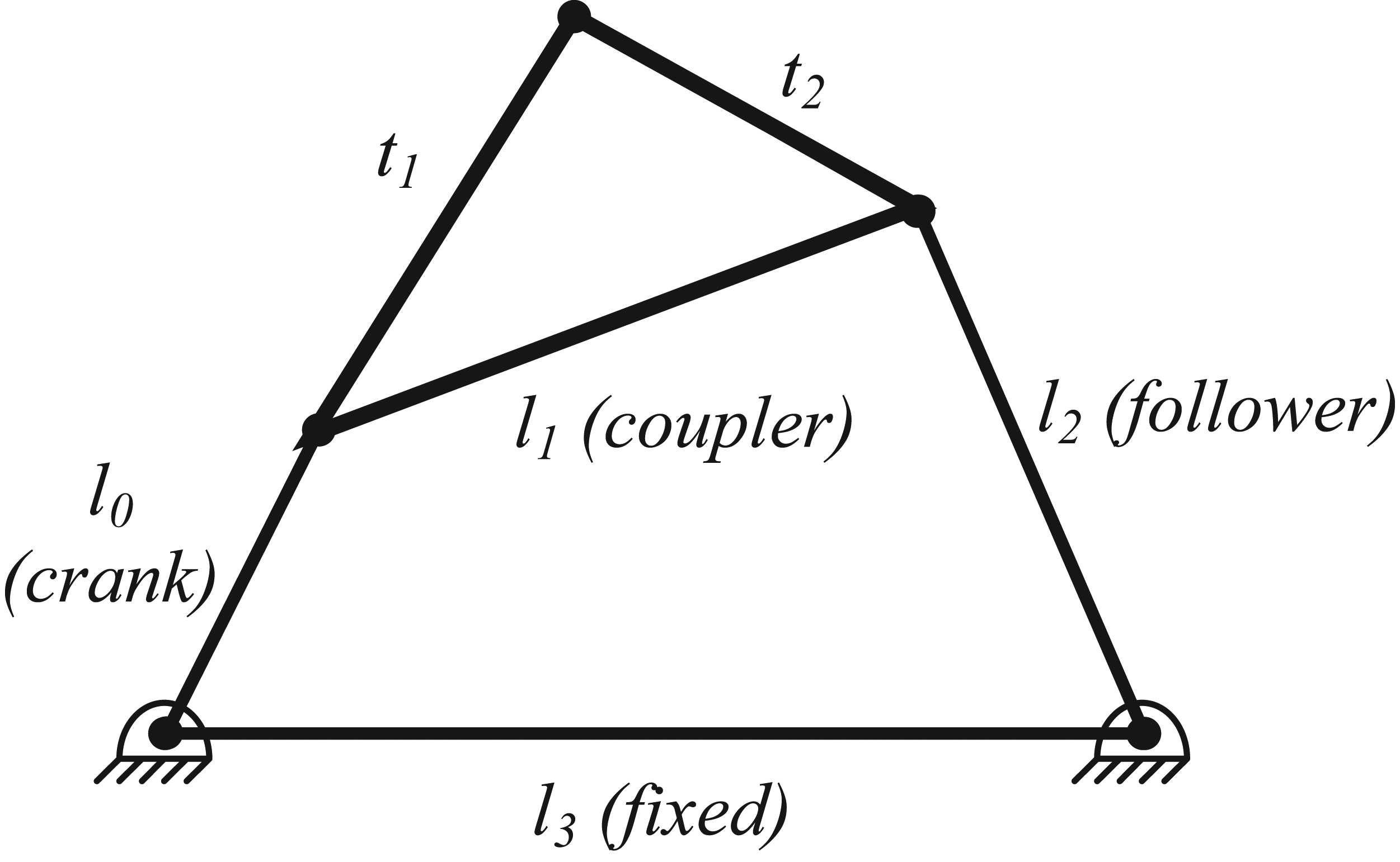
Simple 4 bar linkage mechanism.
It is assumed that the 4-bar linkage mechanism is designed to trace a particular pattern and hence the mechanism is deemed to have failed if its current traced path deviates from the desired path.
In the next section, the ‘design for self-repairing’ process is outlined for a 4-bar link mechanism. The subsequent case studies section presents the process of applying this to a 4-bar link mechanism that has experienced a fault over a number of the self-repairing process steps, before concluding remarks are provided.
Methodology: application of ‘design for self-repairing’ to a 4-bar mechanism
Productive and efficient design is a critical segment of the product lifecycle, and various methodologies have been proposed to enhance this. One such methodology is ‘design for X’, which is a philosophy intended to focus a design around a particular parameter. 14 In this article, the proposed philosophy is ‘design for self-repairing’, which inherently covers a number of other parameters such as ‘design for reliability’ or even ‘design for maintenance’ in that the system must be designed to be self-aware, and hence, the maintenance can shift from being reactive to preventative. The final aim of such an approach is to remove the need for maintenance altogether. To demonstrate this, the steps previously stated are broken down and applied to a 4-bar linkage mechanism.
Cause of fault
It has already been stated that the cause of fault should not be the primary focus when designing a self-repairing system, but nevertheless, it can serve as a useful tool in determining where faults can manifest. In the 4-bar mechanism considered here, a particular rod or element’s dimension could be altered due to shock loading, manufacture defect, thermal expansion and so on. The specific cause of the change in mechanism dimensions is irrelevant – the significant factor is that a change in mechanism dimensions will lead to a change in the behaviour of the system. In addition to the cause is the scope and scale of the fault, particularly in relation to its effect on the function of the system. As a guide for designers when looking to build and integrate a self-repairing schema, common faults that manifest in a particular design, component or system should be accounted for at the design stage where possible. In our example, the loss of function of the tracer element through alteration in the 4-bar mechanism structure can result from an alteration to the element dimension or free play within the joint connectors. Anticipating that these areas are common to loss of function through the act of some form of damage or defect can lead designers to focus upon self-repairing solutions that perform corrective actions that act upon or mitigate this damaged area. For this case study, it is simply assumed that one or more of the rigid elements change its length, and why it occurred does not need to be considered here.
Detection
Perhaps, the best way of detecting a fault is to look for a deviation in the prescribed behaviour, which can be achieved by utilising either internal or external telemetric data. Existing technology already allows for a number of externalised or embedded sensors and a number of high-end industries such as motorsport and aerospace have already began to implement this. By utilising these sensors, the health and status of a system can be continuously monitored, with any deviation in expected behaviour used to identify that a fault has occurred.
The manifestation of failure within a 4-bar linkage mechanism could perhaps be most easily interpreted as a deviation from the prescribed tracer pattern. Hence, it is assumed for this example that the system is aware of the tracer path, but not of a change in element dimensions.
Diagnosis
While the detection of faults could be considered within the realms of current technology, the autonomous diagnosis of a fault is perhaps a more difficult concept. An analogy for this is that any user could potentially tell whether something has gone wrong, but it often requires the input of an expert to say why. One of the reasons for this is the difficulty in validating large, complex system models that can exhibit a vast number of possible states. 11
Current methods for diagnosis include the following:
Model-based: abductive reasoning: compare observation with predicted observation – I expect ‘X’ but get ‘Y’, therefore I must correct ‘Y’ to get it to match;
Bayesian belief networks: probabilistic graphical model (or statistical model) that represents a set of random variables and their conditional dependencies: if ‘X’ and ‘Y’ happen, it is likely a failure with ‘Z’;
Case-based reasoning methods: anecdotal evidence, if ‘X’ happens, do ‘Y’ (simplest, but only accounts for expected failure).
Since a precise mathematical relationship exists between the element dimensions and the tracer pattern, the most obvious choice for a 4-bar linkage mechanism is model-based reasoning. It is assumed that the system knows that the tracer pattern is no longer following the designed trajectory, so now it must infer the most likely point of failure(s) based purely on the information available.
Confirmation of diagnosis
One might reasonably ask whether the fourth step, confirmation of the diagnosis, is required. To demonstrate the importance of this step, an analogy of a car repair is proposed. Currently, the on-board diagnostic systems can present the most likely fault (as a fault code) given the available sensor data; however, it is left to the mechanic to
Look at the indicated faulty part to confirm whether it is indeed ‘broken’;
Recreate the fault to confirm the diagnosis;
Use additional tools (multi-meter, etc.) to pinpoint the precise fault.
It would seem rather ridiculous for the mechanic to blindly rely on the fault code to instigate a particular action without confirmation. In many cases the confirmation of the diagnosis is the step that currently takes the longest to perform manually and consequently has significant room for improvement. Furthermore, there is an issue of confidence in diagnosis, that is, how much certainty must be present to initiate a corrective action? If the initial diagnosis is incorrect, this can lead to undesirable situations such as ‘good’ components being unnecessarily removed or bypassed. Both steps 3 and 4 are important, as they differentiate the self-repairing strategy proposed to design characteristics such as ‘robustness’ which act only to mitigate damage rather than diagnose and repair it.
For the 4-bar linkage mechanism, the confirmation of the diagnosis could be as simple as manipulating one of the controllable elements to determine whether the diagnosis is correct. If it is found to be incorrect, then it must revisit the initial diagnosis and choose from the next most probable point of failure.
Corrective action
The difference between self-healing and self-repair as discussed is open to interpretation, but it is assumed here that the primary difference can be defined by the action that takes place to bring the system back to operation. In essence, a self-repairing system is capable of fixing a given fault to continue satisfactory operation, whereas a self-healing system has the ability to physically bring itself back to an initial state after a fault has occurred. 12
A simple example of a self-repairing strategy is having adaptable redundant components that are able to alter their function to stand-in for whichever component is diagnosed as a fault. This concept of ‘self-repairing through self-reconfiguration’ does not necessarily require additional redundant materials; instead, performance could be sacrificed to ensure continued functionality utilising only the currently available resources. This approach would use degenerate modules that have the ability to perform the same function or yield the same output even if they are structurally different. 15
If it is assumed that there is a failure in an element, then it can be reasonably assumed that we do not wish to affect these further. Therefore, it is preferable to change only the attached ‘tool’– in this case, a simple pen designed to draw a particular pattern. Hence, once the system has been remodelled with revised dimensions, it can then attempt to return back to original desired path through changing dimensions of tracer element (t 1 and t 1 in Figure 1). An alternative approach would have a system with open variables (e.g. through the use of linear actuators) that would enable the system to alter the mechanism dimensions, such as the link lengths. While this would reduce the innate reliability of each component, it would allow far more control over the desired output and therefore corrective action. The results in the following section will analyse both approaches.
Problem domain and case studies
Damage and subsequent faults or failure can occur in complex mechanical systems from a number of sources and result in a varying degree of loss of function or characteristic change in expected output. In the 4-bar linkage mechanism described in the previous sections, this failure or loss of function can result from the consequence of failure in one or more of the linkage bars that make up the system. The self-repairing process outlined previously consists of many steps before a corrective action is even taken, each one important to the success of the overall operation. As a result, a number of case studies are outlined which discuss and demonstrate how a number of these steps can be undertaken for a 4-bar linkage mechanism. First, the need to diagnose the fault within the system using the information available, which in this instance means inferring the point of failure from the current damaged tracer path. Second, the case-study focuses upon confirmation of this diagnosis, while the final case-study looks at a series of solutions for implementing some form of corrective action to regain system function.
Case study: diagnosis
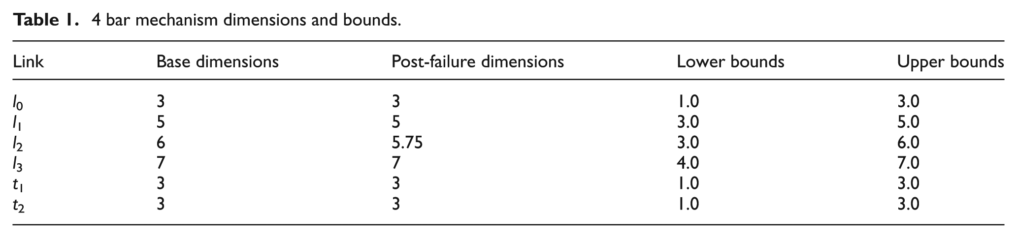
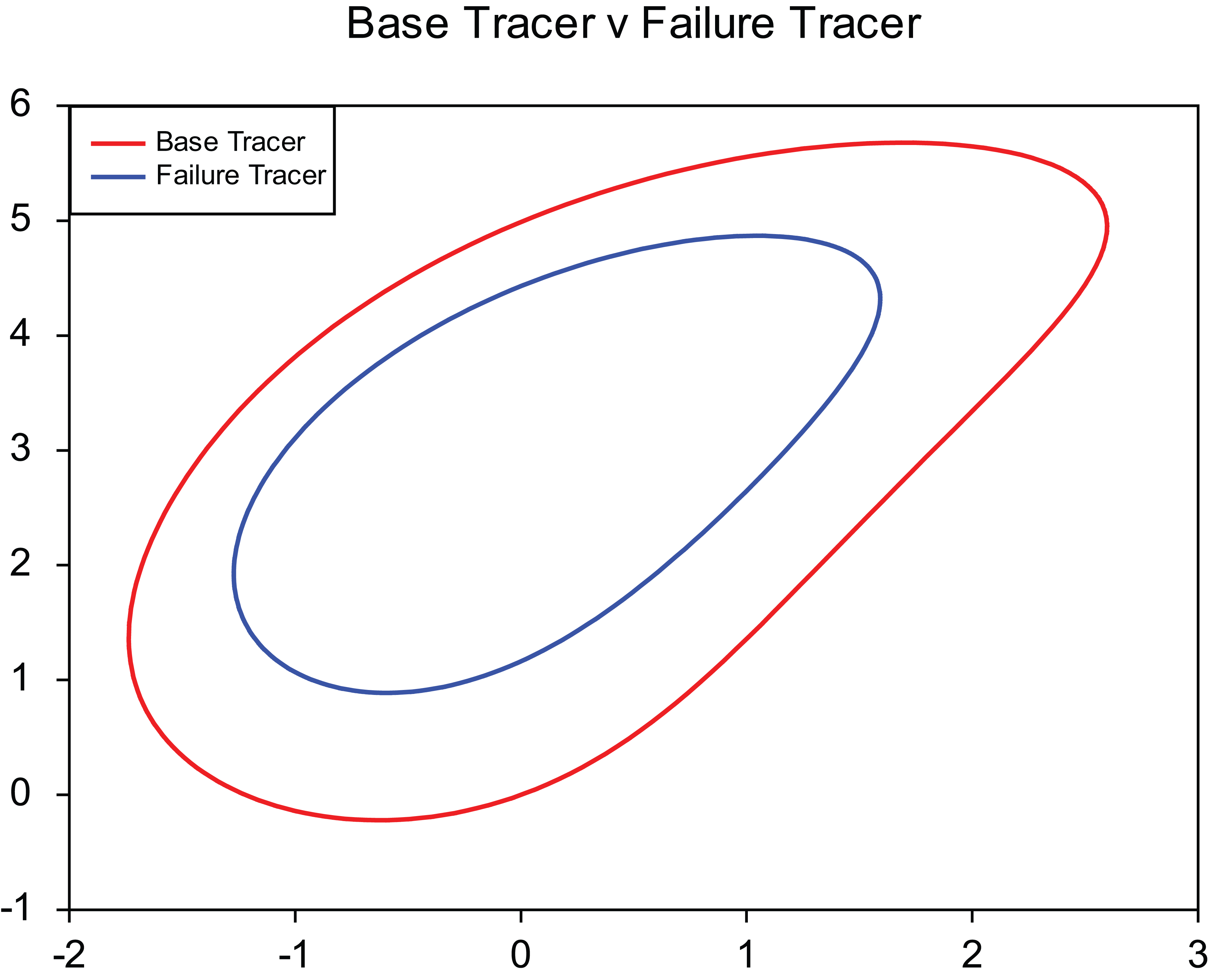
Before any corrective action can be taken, it is important to be able to gauge the extent, degree and position of damage. Under the assumption, the system has detected damage through information on the change in the original tracer pattern that it can begin to infer the source of the failure. Outlined in Table 1 are the base dimensions for the 4-bar linkage mechanism along with the post failure values, in this case a simple reduction in l 2, while a comparison of the base and failed tracer paths is given in Figure 2.
4 bar mechanism dimensions and bounds.
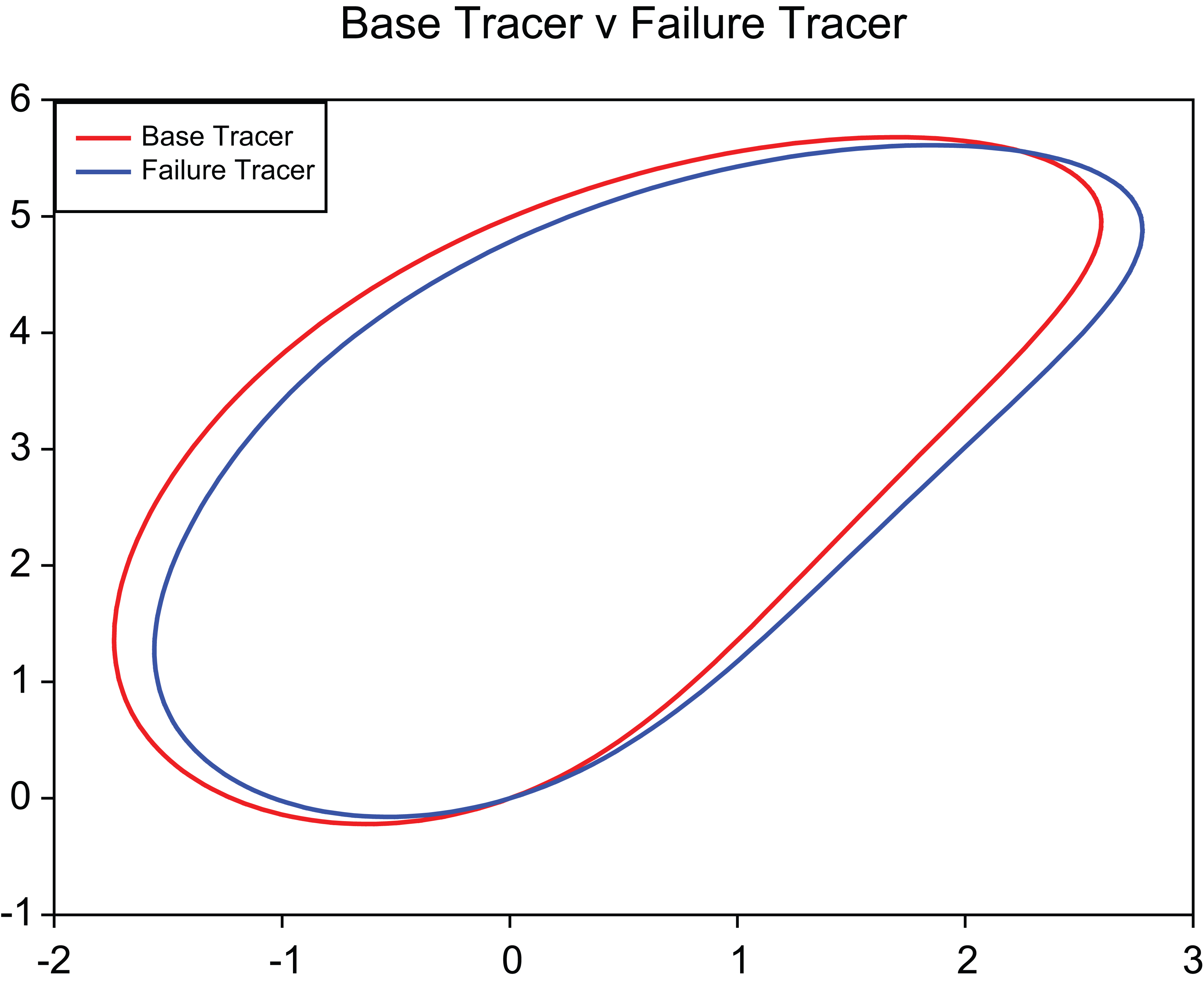
Comparison of 4 bar tracer mechanism paths for initial (red) and damaged (blue) tracer.
In order to diagnose the source of the fault (i.e. which element is responsible), one solution is to replicate the new failed tracer path through an incremental change of the linkage length values that make up the entire 4 bar linkage mechanism. In essence, the self-repairing process can explore the design space of the 4-bar mechanism to try and derive a solution which matches the current failed tracer path and infer the current dimensions as a result. This assumes that there is a one to one matching between the current failed tracer path and its dimensions, and that there exist no other possible dimensions, which could give rise to the same failed tracer path (i.e. every tracer path has a single, unique set of element dimensions that will produce it).
Perhaps the most suitable class of algorithms capable of searching this type of design space are those that utilise local gradient-based optimisation, such as the Nelder–Mead simplex algorithm. 16 Using local information taken from a single solution or design, it is capable of deriving a search direction and generating new solutions that may prove to be more optimal. To demonstrate the process of diagnosis, the Nelder–Mead algorithm was applied to the base design in order to diagnose the source of the original fault that gives rise to the current failed tracer path. Using a single solution over the course of 1500 functional evaluations, the Nelder–Mead algorithm acts upon all the open design variables within Table 1 to find a solution (design dimensions), which matches the failed tracer path in order to evaluate each new design a simple objective looks to minimise the deviation between the current failed tracer path and the new solution tracer path. This is calculated as the average of the Euclidean distance between each point on the tracer path at intervals of 1° changes in the input angle α, as shown in Figure 3.
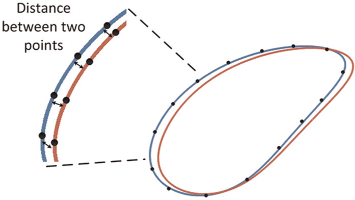
Euclidean distance between tracer path points.
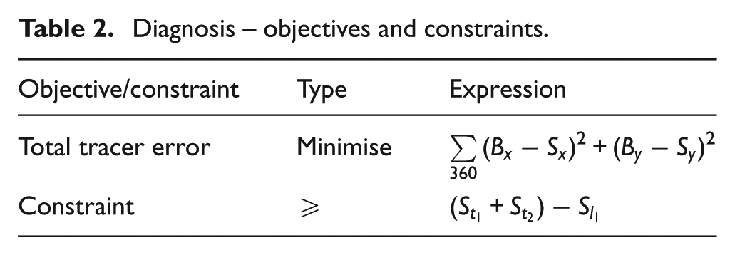
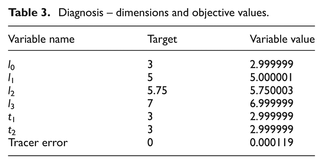
In addition, a single constraint is used to ensure the tracer element lengths remain in contact, and both objective and constraint information are listed in Table 2. The final solution dimensions are shown in Table 3 and match the failed dimensions exactly showing the ability for the algorithm to diagnose what is the source of failure in this instance.
Diagnosis – objectives and constraints.
Diagnosis – dimensions and objective values.
Case study: confirmation of diagnosis
The confirmation of diagnosis is a critical step in the self-repairing process as any changes to the systems with open variables as a result of the corrective action must not further degrade the systems function. There is also a possibility that error is simply carried over and any information from the previous steps passed on or utilised during corrective action may result in the wrong action being taken. If an assessment from the previous diagnosis step was incorrect and future corrective actions alter variables, particularly those deemed as damaged or failed, this could lead to further system failure.
In the simple case study used in this article with only a single point of failure, the algorithm was able to find the precise single solution on every occasion. With more advanced applications such as robotics or multiple simultaneous point of failure, this is not always the case. Furthermore, depending on the computational power and time available, the algorithm can provide a close, but not precise predictions for the failed dimensions. In these situations, a trade-off has to be made between accuracy and computational demand, and if an inaccurate prediction is used, then the system will have to confirm the result before attempting any correction.
To simulate this step, the system was artificially provided with the wrong failure point. It then systematically manipulated one of its controllable elements to determine whether the diagnosis was correct. Ideally in this situation, the system would not have to complete a full motion range check to confirm the diagnosis, so only 10° of rotation of the input link was allowed. Even with this partial knowledge, the algorithm was able to determine that the initial diagnosis was incorrect and hence it returned to the diagnosis stage to seek an alternative solution. The use of a quarantine or tabu list 17 prevented the algorithm from suggesting the same solutions again. By utilising this step and only partial range checking, further damage to the system can be minimised or eliminated.
Case study: corrective action
In order to facilitate some level of self-repairing and regain full or partial function, the system has to undergo some level of corrective action. While this builds on and requires information learned from the previous steps, it is the step that is perhaps of most interest. The corrective action can either be deterministic and often integrated into the system at design time, acting almost reactively to the damage or fault that has occurred, or it can be a non-deterministic, online process. In a non-deterministic process, the response or corrective action is directed as a result of information gathered both currently and from the past while some degree of intelligence or heuristic utilises this information to form what is hoped to be an optimal response. For example, let us look at a simple degradation of function from the result of damage to one of the linkage bars (in this instance l 2). A reduction of its size from its base length leads to a change in the tracer path as demonstrated previously in Figure 2. In order to facilitate some level of self-repairing and regain full or partial function, the system has to undergo some level of corrective action. One possible course of action is in the alteration of the physical linkage bars that make up the 4-bar linkage mechanism, so as to alter the current damaged state into a future state which exhibits better functional performance.
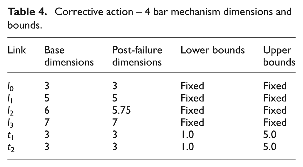
In Figure 4, an example is shown of a mechanism that can alter the tracer element dimensions and alter its output tracer path. By employing an algorithm or heuristic that can calculate the optimal reconfiguration of the dimensions of this mechanism, it is able to recreate the original function of the system, in this case our 4 bar mechanism tracer path. The algorithm chosen to perform this action is again the simple local optimisation Nelder–Mead Simplex method, acting upon the open variables described in Table 4 under the same objectives and constraints used in the previous steps in Table 1 and run with 1000 functional evaluations.
Corrective action − 4 bar mechanism dimensions and bounds.
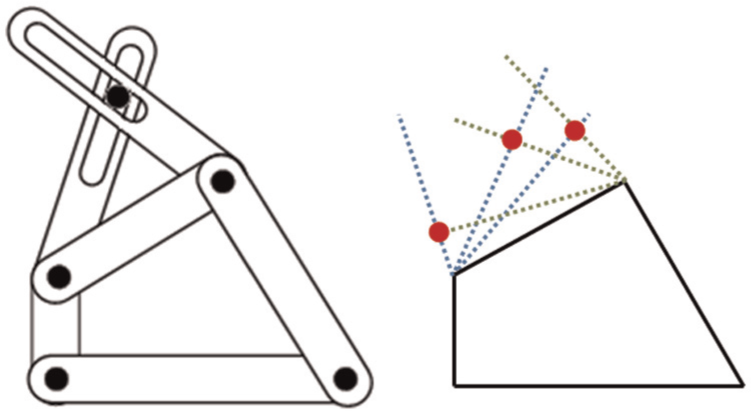
Simple mechanism for varying effective tracer element lengths.
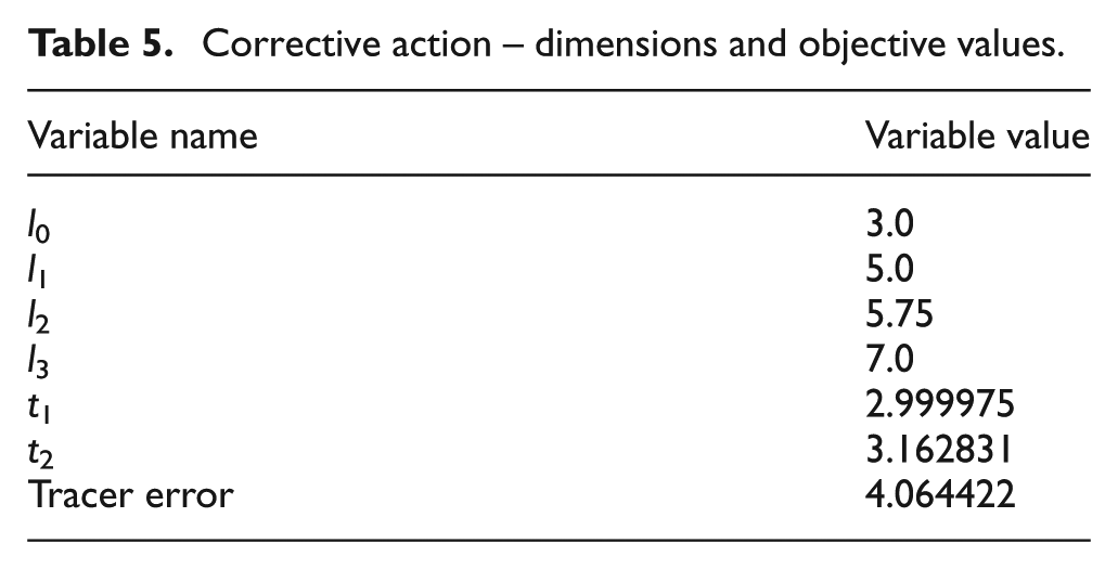
The outcome of such an approach can be seen in both Figures 5 and 6, where the algorithm is able to produce a near optimal reconfiguration of the tracer path. In Figure 5, the solution tracer path is indistinguishable from the original base tracer path as a result of the dimensional changes made by the algorithm on t 1 and t 2 shown in Table 5.
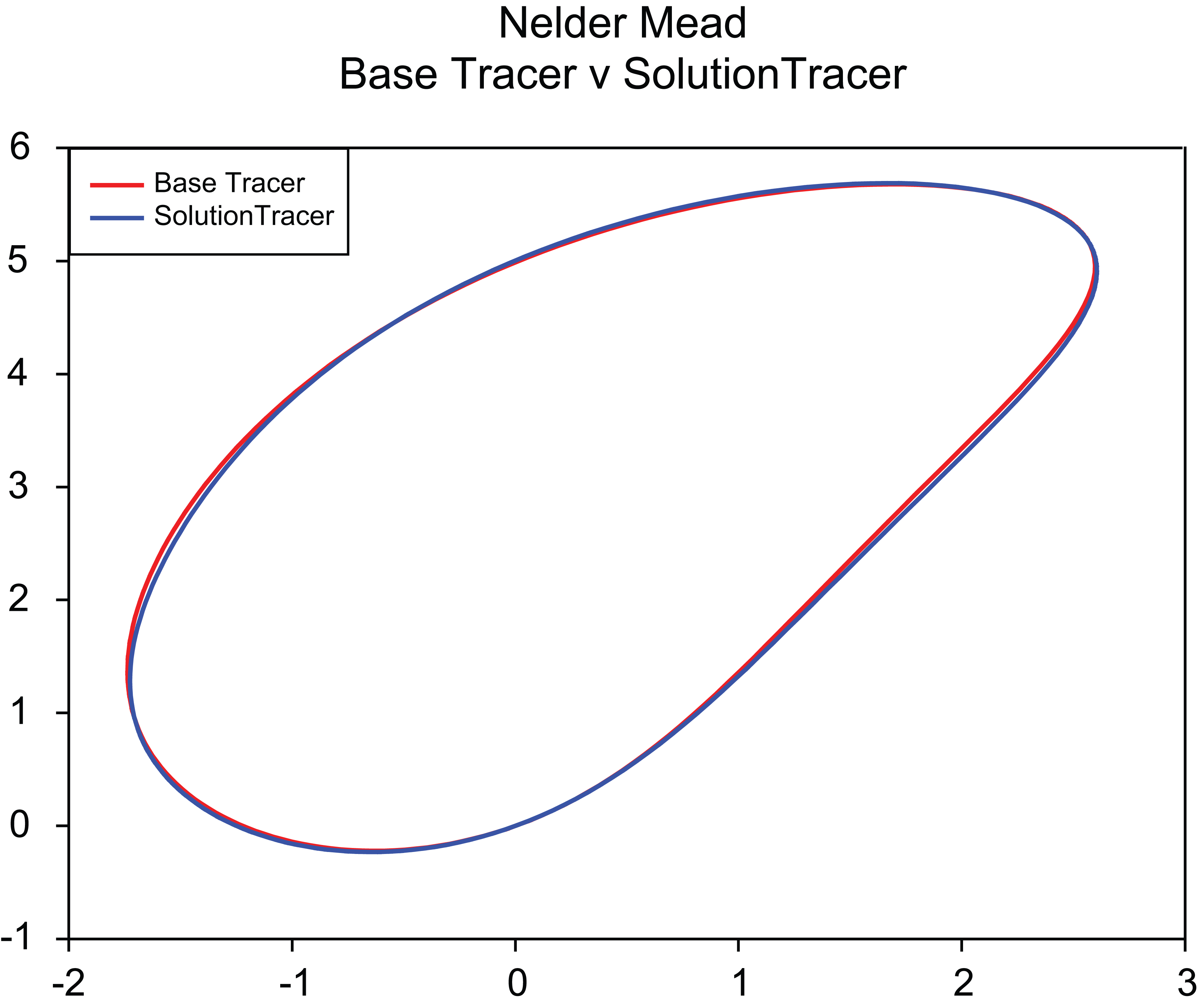
Corrective action – comparison of 4 bar mechanism tracer paths for base (red) and Nelder–Mead fixed solution (blue).
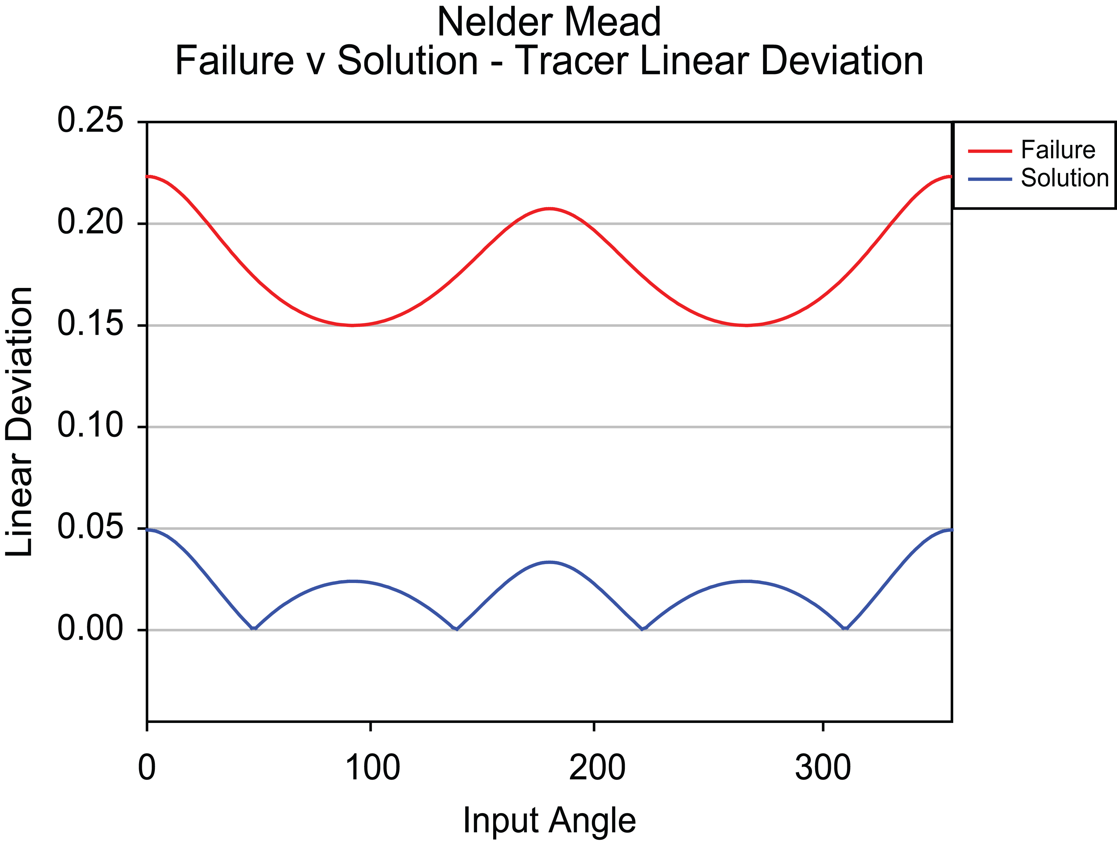
Corrective action – comparison of 4 bar mechanism tracer linear deviation for failure (red) and Nelder–Mead fixed solution (blue).
Corrective action – dimensions and objective values.
Sometimes, alternative objectives are required in order to maintain some degree of functionality even if it is different from the original function. For example, if damage to the 4-bar mechanism was to occur in a different linkage element, in this case l 0 as seen in Table 6, then a tracer shape may arise that the self-repairing process is not able to return to its original path.
Corrective action − 4 bar mechanism dimensions and bounds.
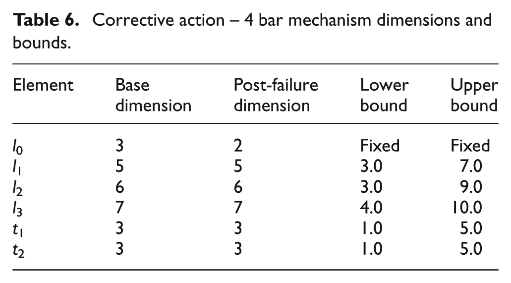
Shown in Figure 7, a comparison between the standard base tracer path and the failed or damage tracer path is considerably larger than our previous examples. Running our standard, Nelder–Mead algorithm using the values in Table 6 to derive a corrective action based upon the same tracer error objectives unfortunately does not yield a very optimal solution as seen in Figure 8, even when we open up more variables to alteration.
Corrective action – comparison of 4 bar tracer mechanism paths for base (red) and damaged (blue) for trajectory example.
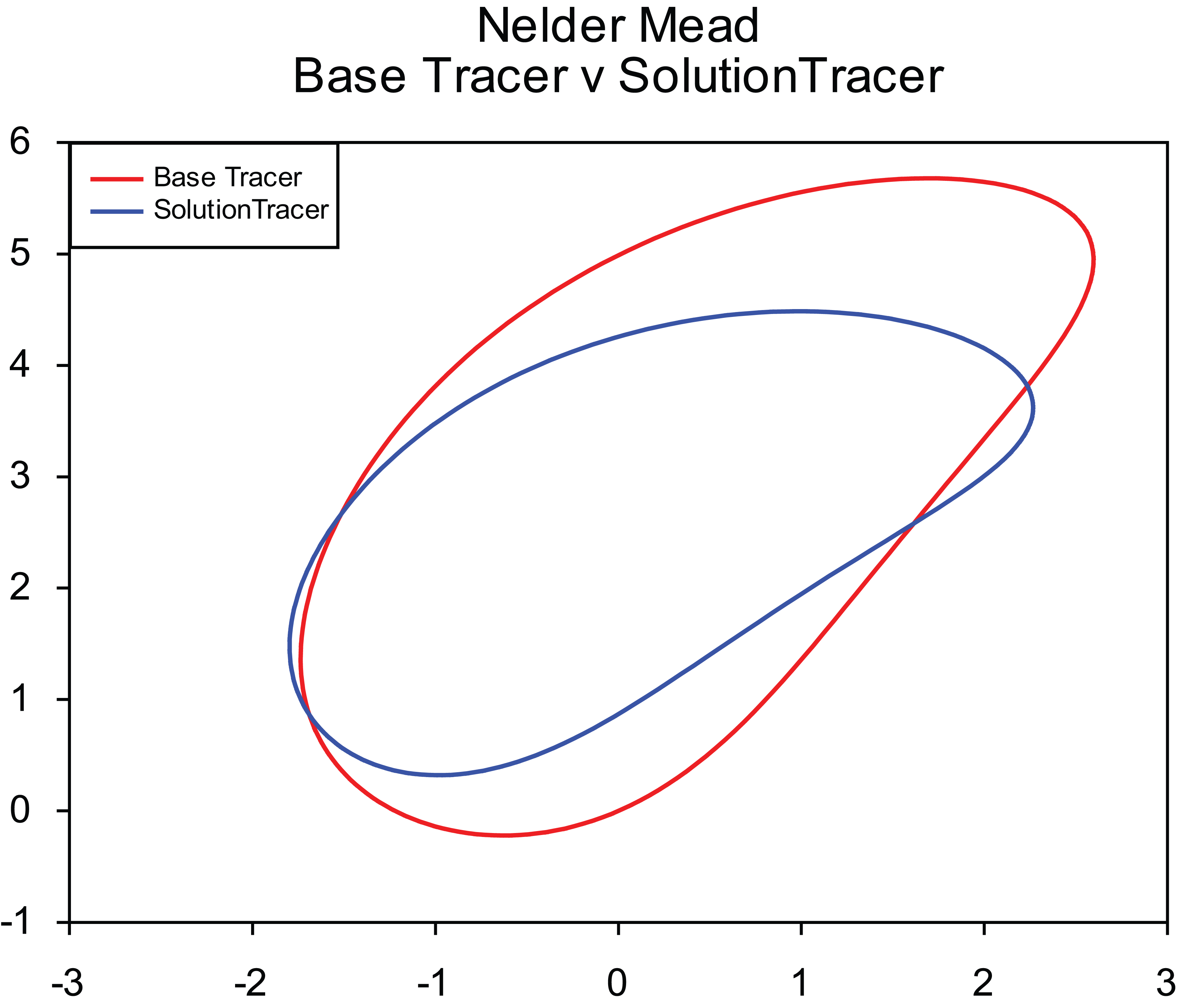
Corrective action – comparison of 4 bar tracer mechanism paths for base (red) and Nelder–Mead solution (blue) tracer for trajectory example.
A different perspective on the overall aim of the corrective action could provide a separate solution that to some degree matches the original function shape but not position. If it is not possible to regain the original tracer path, then perhaps it may be possible to replicate its original trajectory shape. Shown in Figure 9 is a new objective for the self-repairing process to replicate the original tracer trajectory shape regardless of whether it has been translated along one of the axes or has shrunk or grown in ratio to the original tracer path.
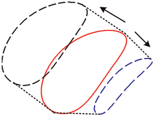
Comparison of tracer path trajectory either through translation or altered ratio/size.
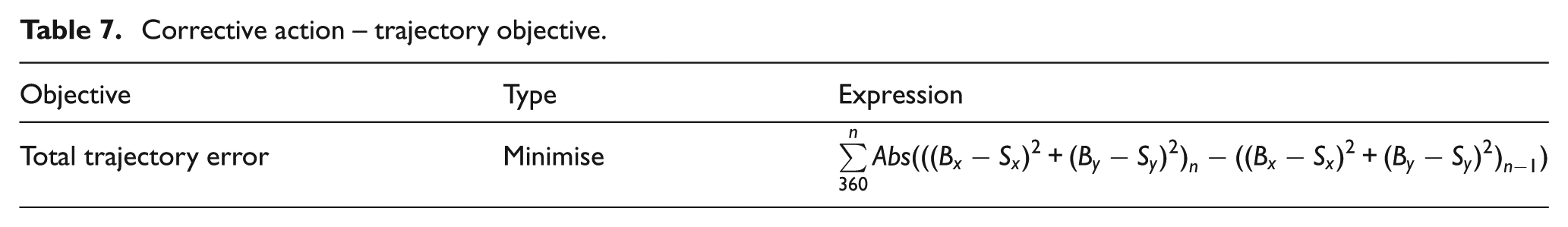
The objective becomes the simple task of minimising the change of deviation from one input angle to the next for all input angles sampled as shown in Table 7. Running the Nelder–Mead algorithm again using the same values as in Table 5, but with this new objective, yields the following solution in Figure 10 and its linear deviation in Figure 11.
Corrective action – trajectory objective.
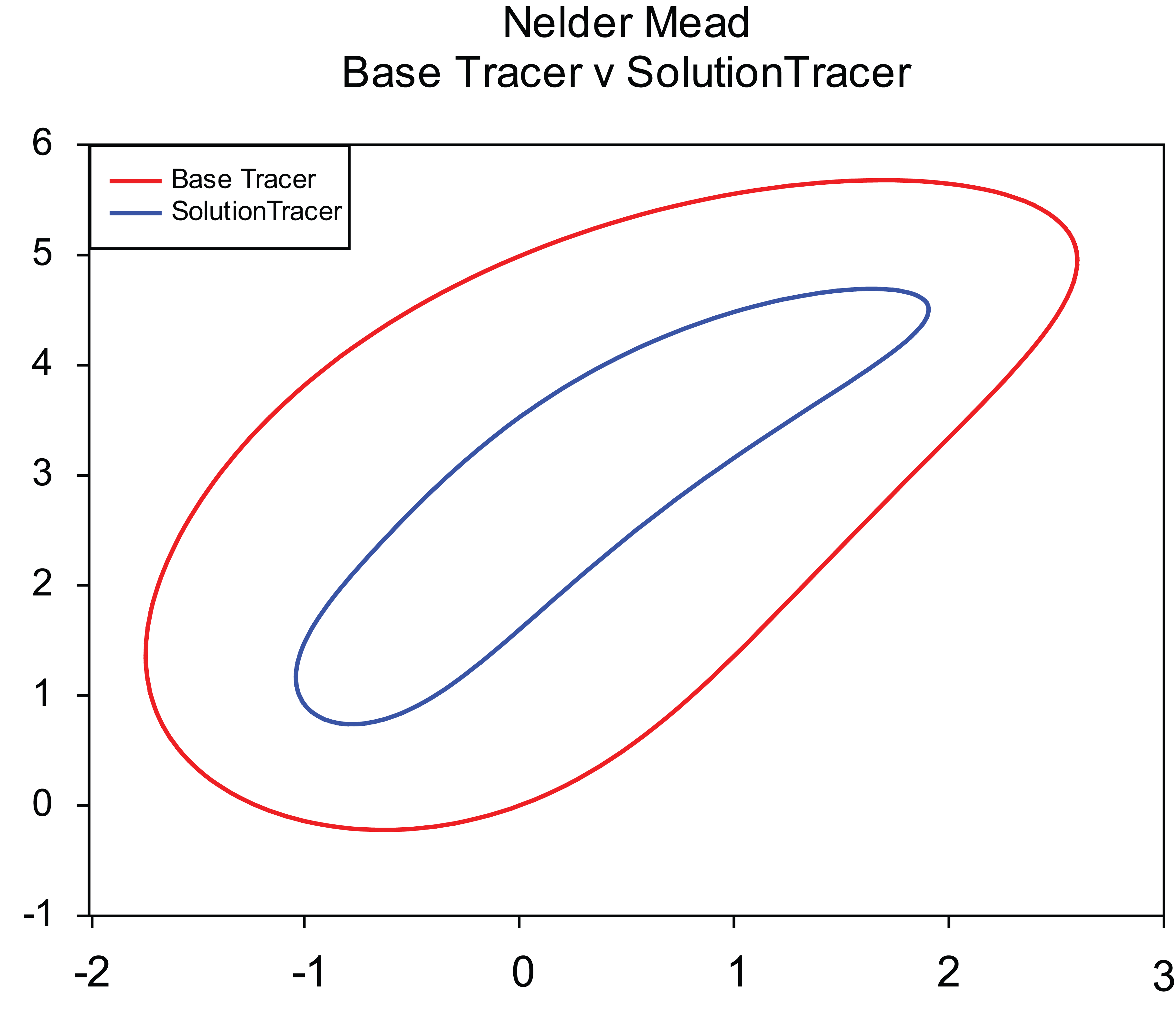
Corrective action – comparison of 4 bar tracer mechanism paths for base (red) and Nelder–Mead solution (blue) for trajectory example.
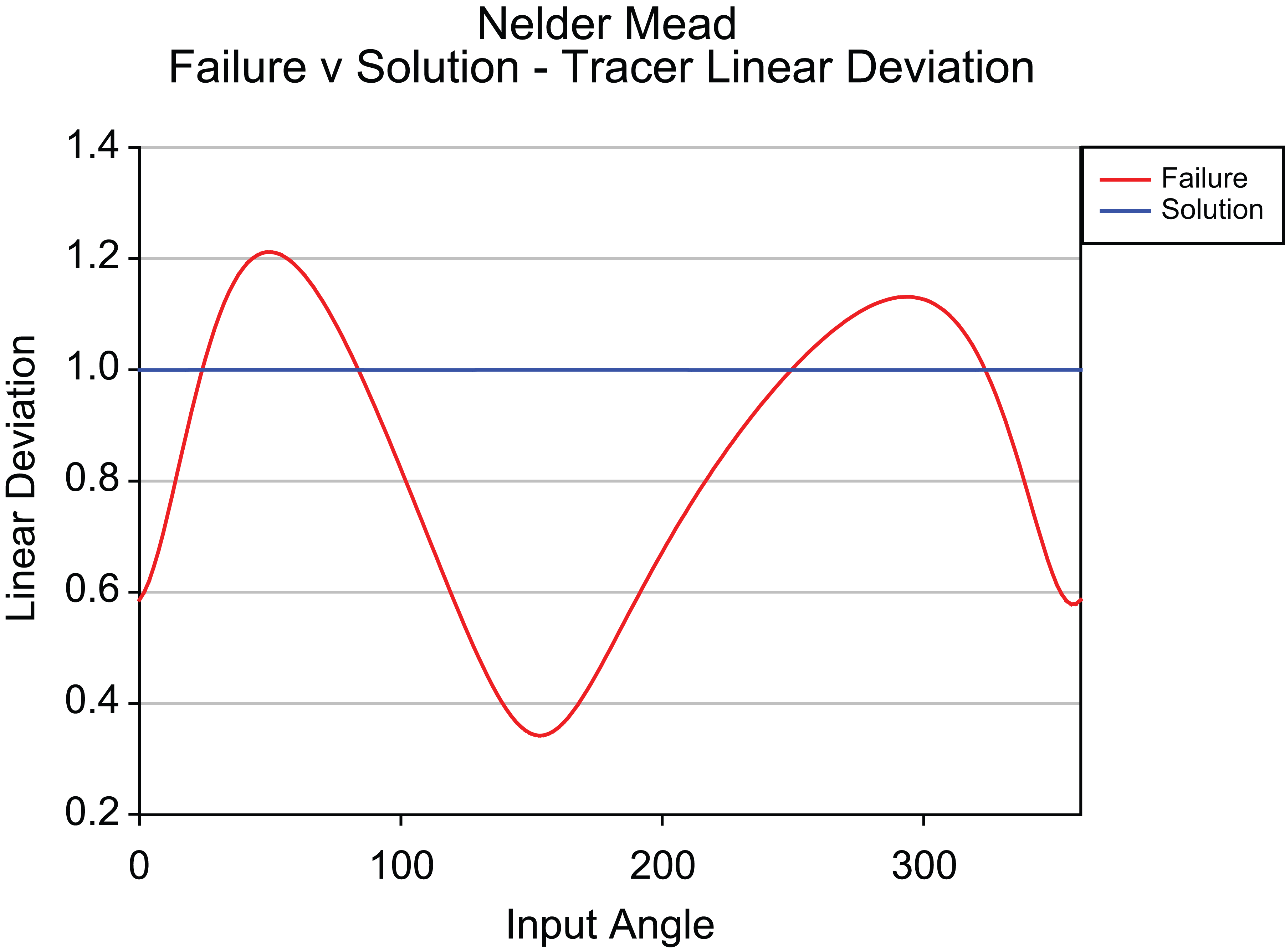
Corrective action – comparison of 4 bar tracer mechanism linear deviation for failure (red) and Nelder–Mead solution (blue) for trajectory example.
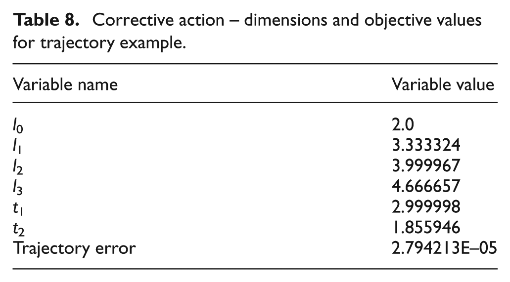
Although containing a higher tracer error, its trajectory is the same shape as the original with each point having the same deviation as the next. The dimensions and objective values are shown in Table 8.
Corrective action – dimensions and objective values for trajectory example.
The examples given previously focus upon a single objective, the need to regain the original tracer path function. However, there may be situations within a particular system that require multiple objectives to be considered when developing the optimal corrective action. For example, in our 4 bar mechanism, the system may wish to account for future damage or faults in conjunction with regaining the original tracer path. Therefore, it may wish to reduce the amount of reconfiguration (dimension change) placed upon the system, while reducing tracer path error. Conversely, the system may wish to act upon two functional objectives, for example, our tracer and trajectory objectives. This is described as a multi-objective problem and is often tackled in one of two ways, the first to combine all objectives into a single weighted ‘sum’ objective function, or to utilise an algorithm which houses multiple solutions or often described as a population of solutions which can be used to form a Pareto set. An example of such an algorithm can be found in the field of evolutionary computation, in a heuristic called non-dominated sorting genetic algorithm II (NSGA-II). 18
This multi-objective genetic algorithm exploits the concept of Pareto optimality in order to partition the population of solutions into a number of ranked sets. This Pareto ranking of a population set works by utilising Pareto dominance to define a set of solutions which either dominate or are equal to all other solutions for each objective within the design problem. The first set to meet these criteria is given a rank and is defined as the Pareto optimal set. The process is repeated for the remaining solutions within the population until all ranks are filled as shown in Figure 12. Here, the two objectives f 1 and f 2 are often antagonistic and work against each other, for example, performance against cost.
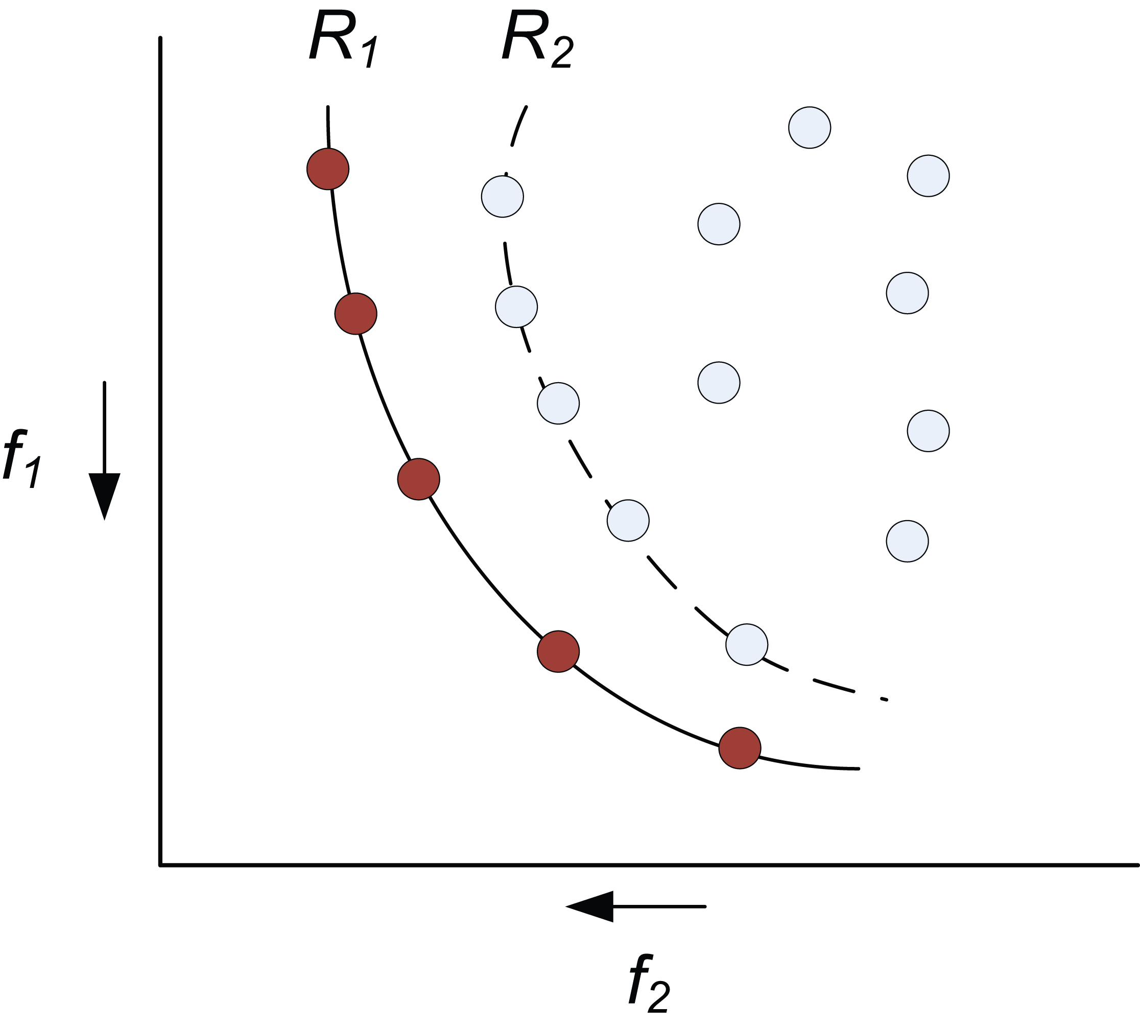
Pareto ranking within a set of solutions.
Applying the multi-objective algorithm to the 4-bar mechanism under the same conditions as described in Table 6 but with both the tracer error and trajectory error objectives allows for a choice of solutions to apply for corrective action. Using the parameters outlined in Table 9, over five separate trials of NSGA-II were able to produce an optimal Pareto set of solutions, the best of which is shown in Figure 13 produced by the first trial.
Default algorithm parameters NSGA-II.
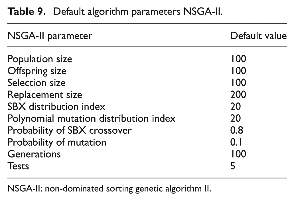
NSGA-II: non-dominated sorting genetic algorithm II.
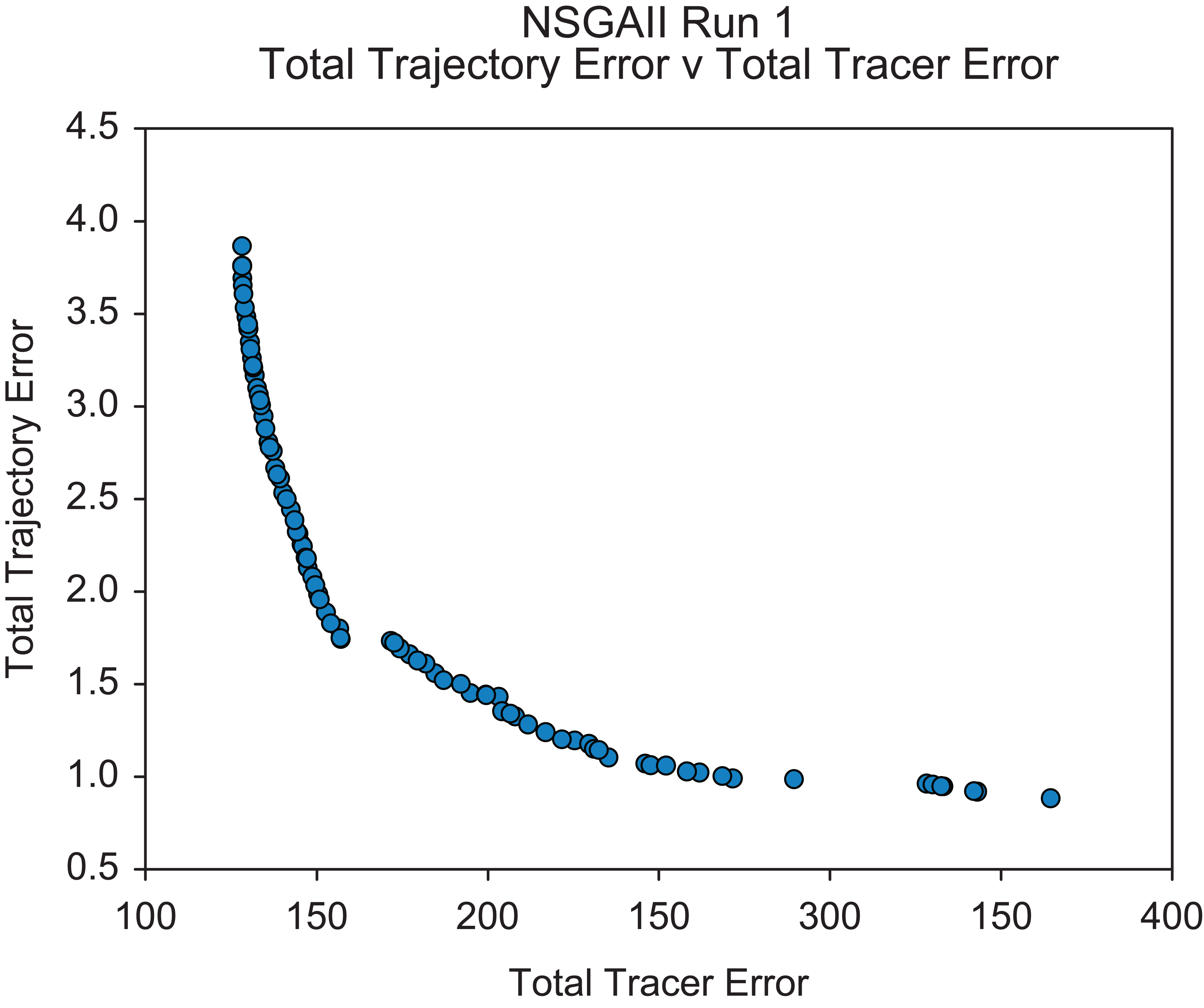
Corrective action – final population set for NSGA-II run 1.
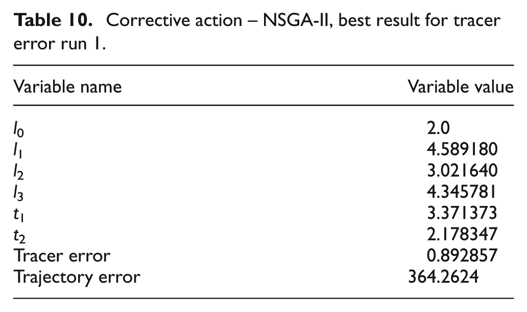
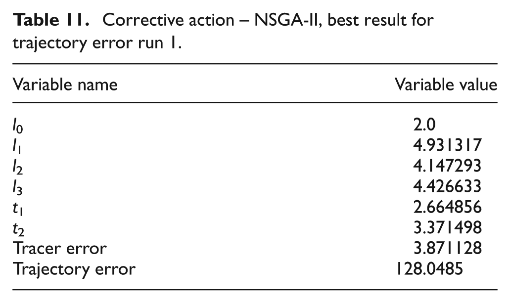
An example of the best solution found for a specific objective is described in Table 10 for the tracer error objective and Table 11 for the trajectory objective. The set of solutions provided give the self-repairing process access to a number of alternative solutions; however, in this instance, there is a loss in optimality. Looking at the best solution found regarding the trajectory objective, it is apparent that it is much worse than the solution found using the single objective Nelder–Mead algorithm shown in Table 8. This is perhaps not surprising considering the heuristic NSGA-II is designed to be more of a global search algorithm providing good but perhaps not optimal solutions, while the local optimisation method is able to significantly improve upon solutions that are found within a local search space. Future work could investigate how to utilise both algorithms in order to gain the ability for more global search and a set of solutions with more powerful local search from the Nelder–Mead algorithm.
Corrective action – NSGA-II, best result for tracer error run 1.
Corrective action – NSGA-II, best result for trajectory error run 1.
Conclusion
Even with extensive planning and fault analysis, it is practically impossible to create a perfectly reliable machine. Current approaches to improving reliability are largely based around advancing areas of modelling and detection to include specific methods designed to overcome particular failure modes. Although this has led to an increase in the operational life of a system and hence improved reliability, it is becoming more and more difficult to predict and mitigate against all possible failure modes. Hence rather than focusing on specific failure modes, a new philosophy is proposed that allows systems to reconfigure themselves to overcome both expected and unexpected failure but focusing on how a failure manifests rather than the failure itself. This approach has been demonstrated in the design of a self-rectifying 4 bar linkage mechanism. This was achieved by breaking the self-repairing process into five individual steps that can be applied to any system, with three of these steps being analysed in more detail.
During this analysis, a number of potential issues were encountered:
Step 0: cause of fault. While the cause of fault should not be of primary concern, it is important to investigate common failure modes as a starting point for subsequent steps. Furthermore, it is important to focus on a system (or sub-system) that has homogeneity among elements. The rectification of a failed motor, for example, would be vastly different from the rectification of a rigid element. If a system has non-homogenous elements, then it should be broken down into sub-systems and each one assessed individually.
Step 1: detection of fault. Perhaps the simplest way of detecting a fault is through user intervention; however, this is not always feasible and somewhat defeats the objective of having a fully autonomous system. The ideal solution is to continuously monitor the desired output of a mechanism or machine to observe any deviation from the status quo. This information can subsequently be used to make an assessment of the damage and monitor the effect of any corrective action;
Step 2: diagnosis of fault. There are several options that can be used to diagnose a fault including probabilistic, model-based or case-based methods. The choice of method will depend on the pre-existing knowledge and complexity of the system. In general, model-based can be preferable, but this can also lead the designer to only focus on particular expected modes of failure. Therefore, it is better to infer the most likely failure mode from a change in output behaviour;
Step 3: confirmation of diagnosis. In simple application or those with known, precise diagnoses, this step can perhaps be ignored. However, in complex systems or those with limited computational resources, it is critical to ensure that any diagnosis made is correct to avoid damaging the system or output further. In these situations rather than seeking a fully confirmed diagnosis, a suspect diagnosis can be used as a starting point to test a possible corrective action. If the system behaves as expected than the diagnosis is confirmed, else the algorithm must tabu the proposed diagnosis and seek another;
Step 4: corrective action. The corrective action is perhaps of most interest to designers as it alone ultimately will govern the extent to which a system is able to recover. Where possible, it is preferable to avoid changes that fundamentally alter the basic system mechanism. For example, in the 4-bar mechanism, it is preferable not to alter the rigid link elements and instead focus on changing the tracer element dimensions. This alone might be sufficient to return the system to near perfect working order, or alternatively as shown in the results, it may be necessary to further alter the system to maintain functionality. Furthermore, it is important to determine what the desired output should be. The results show that if reduced or translated functionality is desired (similar to a ‘limp home’ mode), then a greater degree of failure can be overcome. Maintaining perfect functionality while only manipulating some elements within a system is not always possible and a trade-off has to be made.
Although applied to a simple 4 bar mechanism, the proposed process could be applied to a number of different applications including robotics. In this instance, a manipulator or end effector could develop a fault that limits its motion. By determining the precise limit of motion, the system could determine the most likely point of failure (diagnosis) and then adapt itself stochastically to confirm this diagnosis. Finally, it would utilise other elements within itself to adapt and maintain as wide an operating envelope as possible.
Systems with additional self-repairing mechanisms will inevitably be more complex and hence can become intrinsically less ‘reliable’, even though it has the ability to bring itself back to normal operating conditions. However, in these situations, one must view the system from the perspective of the end-user: a system with an integral resilience-mechanism would appear to be more ‘reliable’– it is able to maintain operation for a longer period of time than would otherwise have been possible – and this should be the primary aim of any self-repairing system.
Footnotes
Declaration of conflicting interests
The author(s) declared no potential conflicts of interest with respect to the research, authorship and/or publication of this article.
Funding
The author(s) disclosed receipt of the following financial support for the research, authorship, and/or publication of this article: The authors would like to thank the EPSRC Centre for Innovative Manufacturing in Through-life Engineering Services (EPSRC Reference: EP/I033246/1) for funding this research.