Sage Journals: Discover world-class research

Abstract

This study proposes an approach that combines a trained neural network with a bisection algorithm to minimize the front end bending of material that occurs during plate rolling. With finite element analysis of plate rolling, front end bending data set was generated under conditions where the three rolling parameters (percentage reduction, entry material thicknesses, and percentage difference in peripheral speed between the top and bottom work rolls) varied at regular intervals. The finite element model was validated by comparing the computed roll forces, with the ones measured from a pilot plate rolling test. The pilot hot plate rolling test, wherein the rotational speeds/rates of two work rolls were independently controlled, was also performed, to validate the proposed approach. The proposed approach predicted the percentage difference in peripheral speed that minimized front end bending of the rolled material within 1 s. When the percentage difference in peripheral speed determined for the selected reduction and entry material thicknesses were input, the measured front end bending was only up to about 5 mm, which is negligible value because the ratio of the front end bending to roll diameter in the pilot plate rolling mill is only 0.0071 (5/700 mm), which is much lower than the ratio (0.02) in an actual plate rolling mill.

Keywords

Front end bending plate rolling neural network rolling test

Introduction

In the plate rolling process, a slab traverses back and forth through a stand, and its thickness is reduced by the work rolls. Here, “stand” denotes a unit machine comprising work rolls, backup rolls, screw down device, drive motor, and a housing that contains the aforementioned parts. After many passes (14–22 passes), the slab ultimately reaches a target thickness. Here, a pass denotes a single rolling action, that is, the traversal of the entire slab through the work rolls. After the slab is rolled in the first pass, it is called material.

In plate rolling, asymmetric rolling states, such as the peripheral speed difference of the top and bottom work rolls, and the temperature difference across the material thickness usually occur. Whenever these asymmetric rolling states occur during rolling, the material’s front end gets bent upward or downward in the direction of the length of the material.

In the case where the front end of the material is bent downward, it has a significant impact on the rolls in the guiding table (a conveyer that transports the material to and from the stand). Hence, mill operators prefer the material front end to be bent slightly upward. However, if the material front end is excessively bent upward, it may hit the stripper (a device that removes the water coolant remaining on the upper work roll). These situations inevitably lead to a decrease in the productivity of the plate mill. In this study, the phenomenon wherein the material’s front end bends upward or downward along the material length during rolling is called front end bending (FEB).

Many researchers have investigated the mechanism of FEB. Lu et al.¹ used a mean shape factor to investigate FEB in the roughing mill in strip rolling process, when the diameters of the upper and lower work rolls were different. Philipp et al.² provided a broad overview of FEB behavior during plate rolling. Philipp et al.² also conducted a two-dimensional finite element (FE) analysis and showed that the bending direction (upward or downward) was dependent on the shape factor, and the circumferential speed difference of the upper and lower work rolls. Nilsson³ performed a pilot plate rolling test, to study how the rolling parameters (circumferential speed difference of the upper and lower work rolls, different reduction ratios, and a thermal gradient across the material thickness) affected FEB. Recently, Byon et al.⁴ proposed a method to determine distinct values of FEB and its slope for a specific roll-bite profile. This was done through the introduction of a geometric factor, which was defined as the ratio of the work roll radius to the entry material thickness.

The investigations performed to date^1–4 have focused on accurate predictions of FEB using the FE method and tried to explain the causes and consequences of FEB. One of the main tasks of the engineers in actual plate mills is to develop an in-line control scheme that minimizes FEB, when the material’s front end is bent downward or upward during rolling. Hence, the development of an analytical model that explicitly expresses FEB as a function of the rolling parameters is required. Once such an analytical model is obtained, we can easily determine the values of the rolling parameter that minimize FEB. However, developing an analytical model is almost impossible because during rolling, FEB is strongly coupled with the heat conduction along the arc of contact, and the mechanical properties of the material being rolled. An empirical model has been used, but it has frequently led to large prediction errors.

The application of a neural network (NN) has emerged as an alternative. Chun et al.⁵ used a feed-forward back-propagation network to predict the width deviation of material being rolled and to determine an optimal edging value during broadside rolling in an actual plate mill. Korczak et al.⁶ applied the NN to predict the nonlinear relationship between the chemical composition of a steel, its grain size, cooling rate, and final mechanical properties. Recently, Bagheripoor and Bisadi⁷ applied NN to an actual hot rolling mill, to improve the predictive capability of the roll force and torque models. Rath et al.⁸ developed an artificial neural network (ANN)-based data-driven model, to predict roll force during the plate rolling process. Gudur and Dixit⁹ utilized the NNs to predict the velocity field and location of neutral point of the strip in cold rolling. However, there has been no report that NN has been used to minimize FEB in the plate rolling process. In this article, a new method of controlling the FEB in plate rolling is introduced. Chen et al.¹⁰ adopted the back-propagation NN to minimize FEB phenomenon. The input layer has three variables: material temperature, material entry thickness, and parameter of deformation zone at each pass. They obtained the optimized rolling schedule at different conditions following training NN and applied it to a plate rolling mill. However, material temperature at each pass in an actual plate rolling mill hardly varies unless the discharging temperature of reheating furnace or material class is changed.

A preliminary inspection¹¹ showed that FEB in plate rolling was mainly affected by three rolling parameters: the entry material thickness, reduction ratio, and circumferential speed difference between the upper and lower work rolls. Hereafter, for convenience, the peripheral speed difference between the top and bottom work rolls, and the entry material thickness will be simply called the speed difference, and the material thickness, respectively.

In this study, we propose an approach that minimizes FEB in the plate rolling process, by combining a trained NN with a bisection algorithm. The inputs of the trained NN are the three rolling parameters mentioned above. FEB is the output of the trained NN. The advantage of the proposed approach is that one can control the input values so that the desired output value is achieved. A FE model of the plate rolling was established, and a series of FE simulations were conducted to generate the values of FEB when the three rolling parameters varied as follows: reduction ratios of 10%, 13%, 16%, 19%, 22%, 25%, 28%, and 31%; speed differences of 0%, 1%, 3%, 5%, and 7%; and material thicknesses of 25, 35, 45, 55, and 65 mm.

The FE model was validated through a comparison of the computed roll forces and measurements. A total of 200 (8×5×5) data points obtained from the FE simulation were supplied to the NN as training data. We could predict the speed differences that minimize FEB for arbitrary values of the reduction ratio and entry material thickness using the trained NN coupled with the bisection algorithm.¹² Note that regulating the peripheral speeds on the top and bottom work rolls is the easiest way to control FEB at a production site. The pilot hot plate rolling test was performed to confirm whether the predicted percentage difference in speed minimized FEB for a given percentage reduction and material thickness.

Experiment

Pilot plate rolling mill and specimen

The rolling experiment was performed using a single-stand, two-high pilot rolling mill, driven by two constant torque AC motors of 350 kW power each, at the Technical Research Laboratory of Hyundai Steel Co. in Korea. The pilot rolling mill has a roller table, similar to the guiding table in an actual plate rolling mill. The pilot rolling mill has a maximum torque of 10.5 kN m. The dimensions of the work roll are 700 mm diameter and 400 mm barrel length. Two AC motors independently drive the top and bottom work rolls.

Board-shaped material was cut from a plate product with the chemical composition of Fe with 0.15 wt% C, 1.35 wt% Mn, 0.4 wt% Si, and 0.03 wt% Al. Its yield stress and ultimate tensile stress are 315 and 490 MPa, respectively. The material was machined into specimen of the dimensions 2 of 20×160 mm (L×W) with a horizontal-type milling machine. Figure 1 shows the photo of the specimen used in the plate rolling experiment. Thickness of the specimens in the pilot plate rolling experiment varied from 25 to 40 mm. As space in the reheating furnace was confined, the specimen length was restricted to 220 mm.

Figure 1.

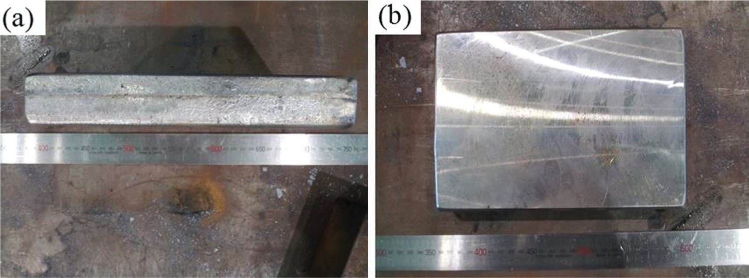
Photograph of the specimen used in plate rolling experiment: (a) side view and (b) top view.

The specimen was soaked in the reheating furnace at 1150 °C for 150 min to ensure homogeneous temperature distribution inside the specimen. As soon as the specimen was taken out of the reheating furnace, the heated specimen began cooling down. Thermocouples (Type K) of 1.6 mm in diameter were embedded in holes of 80.0 mm depth drilled on the side of the specimen to measure the temperature change of the specimen while the specimen was transported via the roller table to the work rolls (Figure 2(a)). The thickness of the specimen in Figure 2(a) is 70 mm, which was the thickness of a test specimen. Before the specimen was fed into the work rolls, metallic oxides on the specimen’s surface were removed manually using a thick metal stick. As we adjusted the speed difference to be either different or equal as required, the material’s front end was bent upward or downward. The speed difference in this study was defined as follows

Δ v = \frac{v_{L}^{R} - v_{U}^{R}}{v_{L}^{R}} \times 100

(1)

Figure 2.

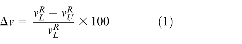
A life-size photograph of pilot plate rolling testing: (a) the heated material (specimen) is moving on the roller table (guiding table) up to ahead of the work rolls. Three thermocouples are embedded in the material (viewed at the entry side) and (b) the material is being rolled between the work rolls (viewed at the exit side).

Here, $v_{L}^{R}$ and $v_{U}^{R}$ are the peripheral speeds of the bottom (lower) and top (upper) work rolls, respectively. Figure 2(b) shows the specimen being deformed between the work rolls. No lubricant was applied to the surface of work rolls during the rolling test.

Measurement of FEB

The radius of curvature of the material front end was adopted as a measure of the upward or downward bending of the material front end, that is, FEB.² This measurement method is advantageous only if the specimen (material) is long enough. However, most people have experienced difficulty in determining the magnitude of FEB in terms of the radius of curvature. On the other hand, Jeswiet and Greene¹³ introduced a curl ratio, a measure of the turn-up or turn-down of the material front end. The curl ratio is defined as the ratio of the maximum elevation of the front end of the rolled material to a reference length along the material length direction. The curl ratio is always dependent on the reference material length. If the reference material length is not enough, then the ratio is limited in its usage.

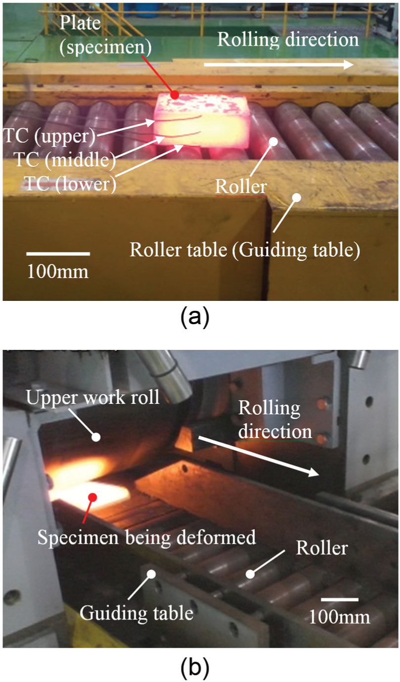
Figure 3 depicts the procedure for measuring FEB that was adopted in this study. First, a tangential line (Line ①), originating at the bottom of the rolled specimen (material), is drawn from the specimen’s rear to its front end. We then draw another line (Line ②), perpendicular to Line ① so that the two lines intersect at a point on the front end of the rolled specimen. In this way, FEB is defined as the distance between the points A and B.

Figure 3.

Side view of material in which FEB occurs for given material thickness, reduction ratio, and peripheral speed difference on the top and bottom work rolls after the pilot plate rolling test: (a) material’s front end is bent upward and (b) material’s front end is bent downward.

FE analysis

Two second-order partial differential equations (an equation for motion of the material being deformed, and an equation for the heat balance of the work roll/material), together with the boundary and initial conditions, are necessary to analyze the hot rolling. FE formulation is obtained by applying a variational method to the equations. FE models of the hot rolling are numerous, depending on how to model the frictional forces between the work roll and the material, and the material deformation behavior at high temperature.

The solution methods of the FE formulation are given in many books.^14–16 In this study, we used the commercial FE code ABAQUS^®, which is suitable for the analysis of the nonlinear elastic–plastic deformation of material during hot rolling, to obtain the solutions.¹⁷ The work rolls were treated as rigid bodies because the effect of the material plastic deformation in the work roll-bite on the elastic deformation of the work rolls is negligible since the specimen width (160 mm) is much smaller than the work roll diameter (700 mm). Hence, two-dimensional thermo-mechanical FE analysis was performed. Temperature variation in the material due to the metallurgical transformations during rolling was not taken into account.

The material is assumed to be isotropic and homogeneous. Element CPE4RT (a four-node plane strain thermally coupled quadrilateral, bilinear displacement and temperature, reduced integration, and hourglass control) was used. We carried out mesh sensitivity analysis and selected element size, 4×4 mm. Appropriate boundary and initial conditions should be introduced to solve these initial boundary value problems.

Boundary conditions

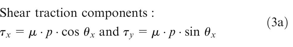
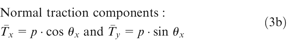
Figure 4 shows the material being deformed between the work rolls. The mechanical boundary condition of the material is as follows. Zero normal and tangential surface traction conditions are prescribed to the boundaries Γ₁–Γ₄, except for the region where it came in contact with the work roll

σ_{n} = 0 and σ_{t} = 0

(2)

Figure 4.

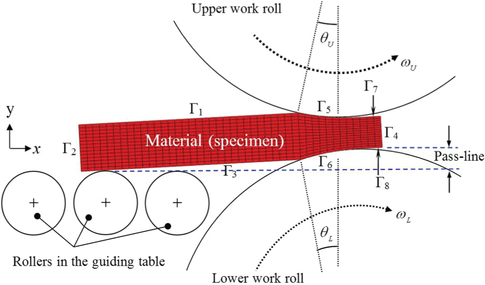
Boundaries on the material being deformed between the work rolls in case that circumferential speed difference between the upper and lower work rolls occurs. Pass-line denotes a distance between the upper vertex of the lower work roll and the underneath of the material entering into the lower work roll. Boundaries Γ₇ and Γ₈ denote the free surface newly generating during rolling.

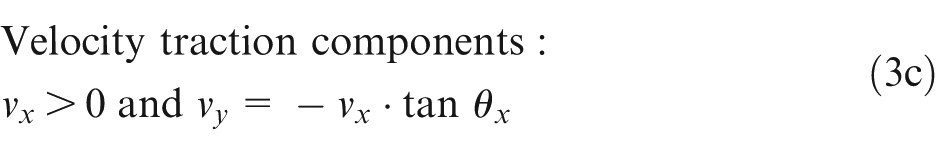
Essential boundary conditions (u_x and u_y ) are applied at the center of the work rolls, such that the displacements along the x and y directions are null. The velocity vector components (v_x , v_y ), shear tractions (τ_x , τ_y ), and normal tractions ( ${\bar{T}}_{x}, {\bar{T}}_{y}$ ) are prescribed along the boundaries Γ₅ and Γ₆, as follows¹⁸

\begin{matrix} Shear traction components : \\ τ_{x} = μ \cdot p \cdot \cos θ_{x} and τ_{y} = μ \cdot p \cdot \sin θ_{x} \end{matrix}

(3a)

\begin{matrix} Normal traction components : \\ {\bar{T}}_{x} = p \cdot \cos θ_{x} and {\bar{T}}_{y} = p \cdot \sin θ_{x} \end{matrix}

(3b)

\begin{matrix} Velocity traction components : \\ v_{x} > 0 and v_{y} = - v_{x} \cdot \tan θ_{x} \end{matrix}

(3c)

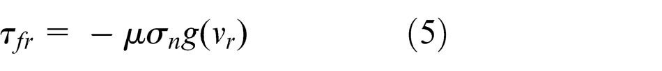
where µ denotes the Coulomb friction coefficient, which was set to 0.35.^19,20 θ_x indicates the angle between the tangent to the work roll-material contact surface and the rolling direction, p is the roll pressure. Note that the values of θ_x and p on Γ₅ are slightly different from those on Γ₆, due to the pass-line, which indicates the distance between the upper vertex of the lower work roll and the underneath of the material entering into the roll gap. Note that during rolling, new free surfaces (i.e. boundaries Γ₇ and Γ₈) are continuously generated. 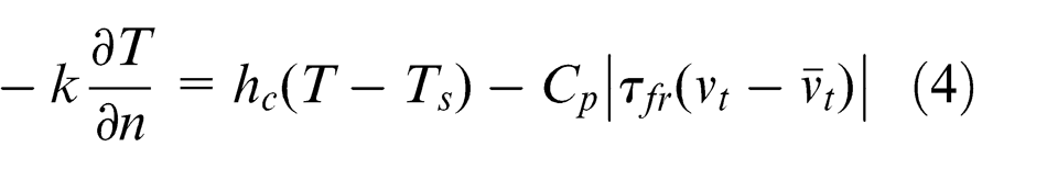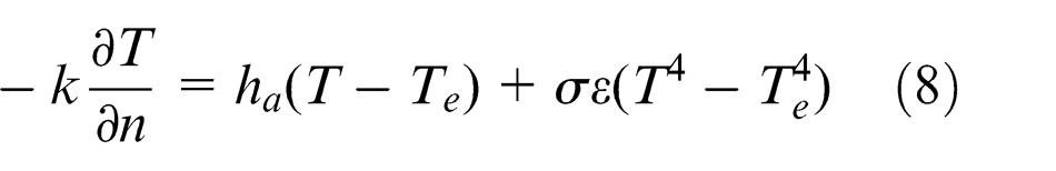Zero tractions and zero mass flow ( $\bar{v} \cdot \bar{n} = 0$ ) are assigned to the boundaries, as well. $\bar{n}$ and $\bar{v}$ indicate unit normal vector and velocity vector, respectively.

Likewise, the thermal boundary conditions on the material are prescribed. At the deformation zone, heat is conducted from the material to the work rolls; and at the same time, heat is generated due to frictional force. Hence, the thermal boundary conditions on Γ₅ and Γ₆ are as follows

- k \frac{\partial T}{\partial n} = h_{c} (T - T_{s}) - C_{p} | τ_{fr} (v_{t} - {\bar{v}}_{t}) |

(4)

where

τ_{fr} = - μ σ_{n} g (v_{r})

(5)

where h_c and T_s are the interface (contact) heat transfer coefficient and the surface temperature of the work roll, respectively. h_c was set to 20 kW m⁻² K⁻¹, which is the value that has been widely used in hot rolling.^21,22 The second term in the right-hand side of equation (4) denotes heat due to the friction between the material and the work roll. C_p in equation (4) denotes the partition coefficient, the local fraction of frictional heat passing into the work rolls.

There have been many studies to determine the value of the partition coefficient. In the case of cold rolling, Wilson et al.²³ studied interface temperatures in the roll gap in cold strip rolling using the heat transfer model which uses finite difference formulation. They assumed that the local fraction of frictional heat passing the work rolls could be calculated using a temperature matching condition. As heat addition in the strip due to plastic deformation is increased, more heat flows from the strip to the work rolls. In case that plastic heating of the strip is dominant, the partition coefficient may be much greater than unity. Chang²⁴ proposed a method for computing temperatures in the strip and work rolls in cold strip rolling to reduce computational time. They reported that the partition coefficient in the slipping region and that in the sticking region are different. They also argued that the partition coefficient might be greater than unity within slipping region where heating due to plastic deformation is dominant.

Meanwhile, variations in the partition coefficient value in hot rolling are different from those in cold rolling since strip temperature during hot rolling is much higher than the work roll temperature. Hatta et al.²⁵ stated that the heat conductivity value of the roll is about twice as large as that of the strip in hot rolling since the temperature of rolls is by far lower than that of the strip. Subsequently, they assumed that the partition coefficient might be 0.6–0.7. Assuming that 60%−70% of frictional heat passes into the work rolls might be plausible. However, considering that the value of the partition coefficient is noticeably dependent on rolling conditions such as cooling condition on the work rolls and roll speed, precision measuring devices and testing machine are required to verify the assumption.

Recently, Legrand et al.²⁶ investigated the roll-bite heat transfer during pilot hot strip rolling using two types of temperature sensors (drilled and slot sensors) together with analytical heat transfer model and finite difference model. They showed that heat flux dissipated by friction was about 10% of the conduction heat flux. In this light, determining the value of the partition coefficient without precision machines and instrument for measuring temperature is not helpful to predict temperature distribution in the work rolls during hot rolling. Hence, in this study, it is assumed that half of the frictional heat flows into the work roll and 50% into the strip. Therefore, the partition coefficient C_p in equation (4) was set to be 0.5. Sun et al.¹⁹ and Na et al.²⁷ also assumed that C_p = 0.5.

$ν_{t}$ and ${\bar{ν}}_{t}$ in equation (4) are the tangential components of the velocity vectors of the material and work roll, respectively. τ_fr , σ_n , and μ in equation (5) are the tangential (friction) stress, normal stress, and the Coulomb friction coefficient, respectively. Hence, v_r is the relative tangential velocity between the strip and the roll. Sticking friction occurs when $| μ σ_{n} |$ is greater than the shear yield stress of the strip. The function g(v_r ) in equation (6) was introduced by Chen and Kobayashi²⁸ to deal with both the sliding and the sticking friction in the contact zone

g (ν_{r}) = - \frac{v_{r}}{| v_{r} |}

(6)

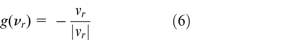
However, for a given normal stress, the tangential (friction) stress in equation (6) has a step function behavior upon the value of v_r . The discontinuity of the value of τ_fr results in no converged solution.

In order to overcome this difficulty, Chen and Kobayashi modified the function g(v_r ) in the following

g (v_{r}) = - \frac{2}{π} \tan^{- 1} \frac{v_{r}}{b}

(7)

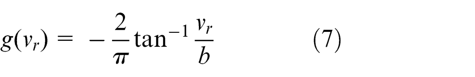
where b is a positive constant, which is several orders less than the roll velocity so that the function g(v_r ) in equation (7) is almost identical to that in equation (6) for $| v_{r} |$ slightly larger than 0. Note that the magnitude of b has almost no effect on the magnitude of tangential (friction) stress if the value of b is several orders less than the roll velocity.^19,28 The role of very small positive number b is to avoid poor convergence.

Heat is lost on Γ₁, Γ₃,Γ₇, and Γ₈, due to radiation and convection to the environment. The thermal boundary conditions are as follows

- k \frac{\partial T}{\partial n} = h_{a} (T - T_{e}) + σ ε (T^{4} - T_{e}^{4})

(8)

where h_a and T_e are the convective heat transfer coefficient in air and the surrounding temperature, respectively. h_a was set to 0.03 kW m⁻² K⁻¹.²⁹ σ and ε are the Stefan–Boltzmann radiation constant of a black body (5.67×10⁻⁸ W m⁻² °C⁻⁴) and the emissivity of the material at a temperature of around 1000 °C (0.8), respectively.

Heat is also lost due to contact between the rolls of the roller table and the underneath of the material, while the material is moved from the reheating furnace to ahead of the work rolls. The thermal boundary condition at the interface between the rolls in the roller table and the bottom of the material is

- k \frac{\partial T}{\partial n} = h_{RT} (T - T_{e})

(9)

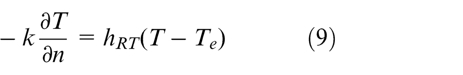
where h_RT is the interface heat transfer coefficient. In order to determine the value of h_RT , a pilot hot plate rolling test was conducted (see section “Pilot plate rolling mill and specimen”).

Figure 5 shows the temperatures measured and computed at three points in the material, while the material discharged from the reheating furnace is moved by the rolls in the roller table up to ahead of the work rolls. As soon as the material touches the roller table, the lower point begins to cool at a faster rate than at the middle and upper points. When the material thickness is 25 mm, the predictive value at the upper point slightly overestimates the measurements. In the case of 35 mm material thickness, some deviations between the predictions and measurements at the middle point are observed at the beginning of the test. However, a good agreement is noted between the predictions and the measurements at the lower point. Based on these measurements, h_RT was determined to be 0.3 kW m⁻² K⁻¹. No-friction condition was enforced at the interface between the rolls in the roller table and the bottom of the material.

Figure 5.

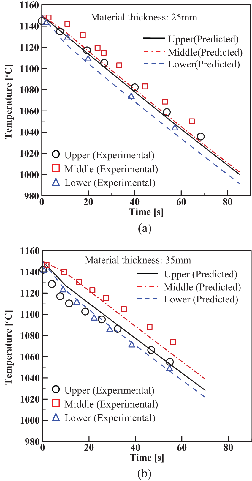
Predicted temperature and measured ones at three points (upper, middle, and lower) for two different material thicknesses. For both cases, reduction ratio is 22% and circumferential speed difference is 0%: (a) entry material thickness, 25 mm and (b) entry material thickness, 35 mm.

Constitutive equation

The accurate prediction of the roll force (torque), heat gain arising from the friction on the contact surface, and heat gain due to plastic deformation during hot rolling mainly depends on the constitutive equation of the specimen (material) at high temperature. The equivalent stress is related to the temperature, strain rate, and strain of the material during rolling. The material used in this study was a low carbon steel (0.15 wt% C). Hence, we selected Shida’s³⁰ constitutive equation that is applicable under the following conditions: carbon content: 0.07%−1.2%; temperature: 700 °C–1200 °C; and strain: ≤0.7, but Shida’s constitutive equation is not applicable for strain rates greater than 100 s⁻¹. The equivalent stress is expressed as follows

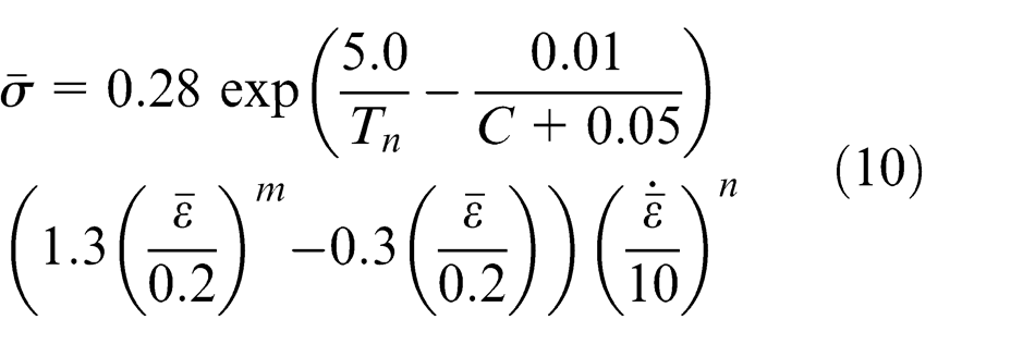
\begin{matrix} \bar{σ} = 0.28 \exp (\frac{5.0}{T_{n}} - \frac{0.01}{C + 0.05}) \\ (1.3 {(\frac{\bar{ε}}{0.2})}^{m} - 0.3 (\frac{\bar{ε}}{0.2})) {(\frac{\overset{\cdot}{\bar{ε}}}{10})}^{n} \end{matrix}

(10)

In the above equation, T_n = (T + 273/1000), where T is the temperature (°C). C, $\bar{ε}$ , and $\overset{\cdot}{\bar{ε}}$ are the equivalent carbon content, strain, and strain rate, respectively. The constants m and n are the strain hardening and strain rate sensitivity coefficients, respectively. These are functions of the carbon content as follows: m = 0.41 − 0.07C and n = (−0.019C + 0.126)T +(0.076C − 0.05).

Neural network

Inputs and output

A preliminary inspection¹¹ showed that the output, that is, FEB in plate rolling was mainly affected by three inputs: the entry material thickness, reduction ratio, and speed difference. Figure 6 shows a schematic of the NN structure employed in this study. It consists of an input layer, three hidden layers, and an output layer. Each layer has a certain number of neurons, which are linked by adjustable weights.

Figure 6.

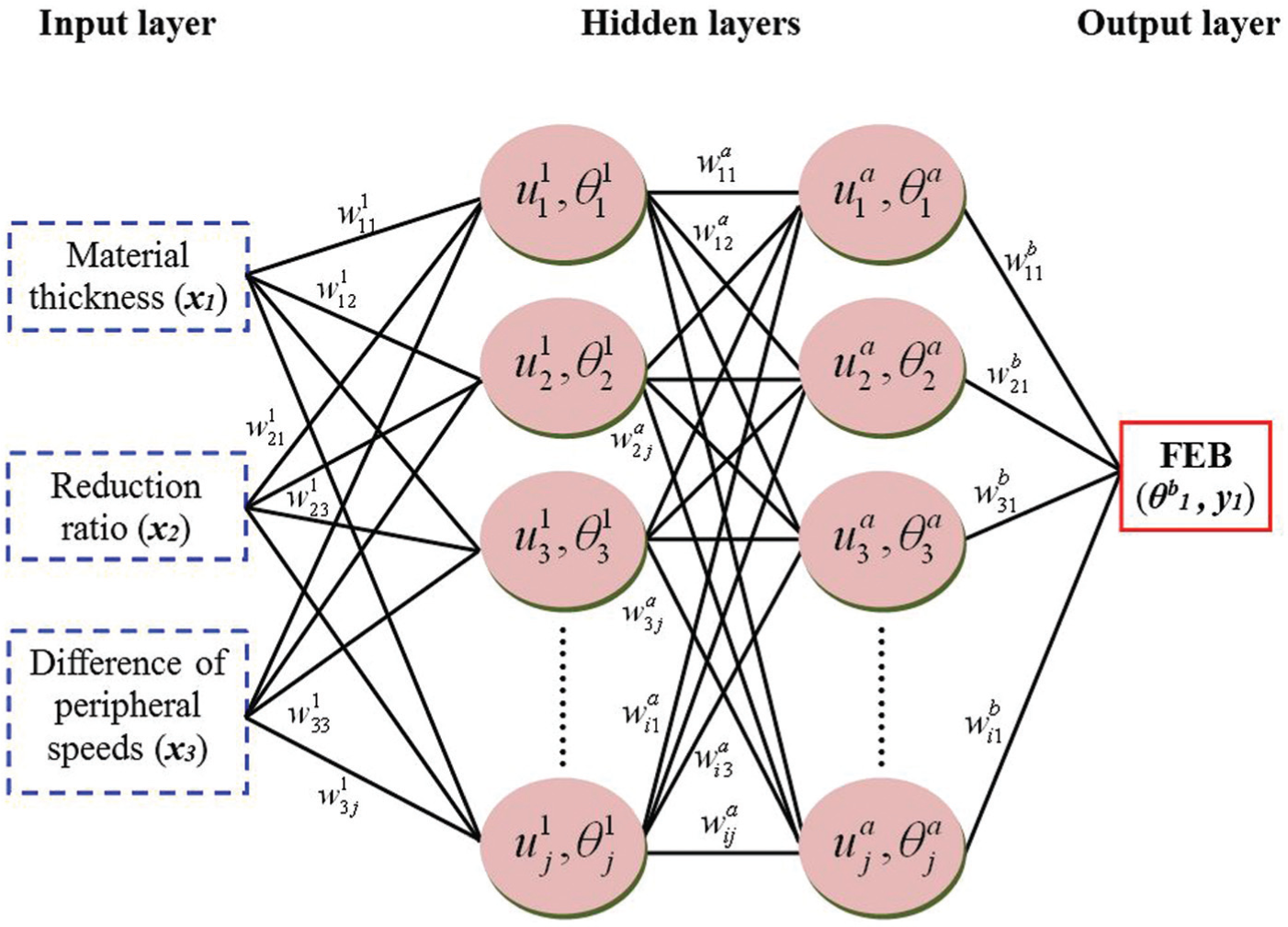
Schematic diagram of multilayer NN structure employed in this study.

Generating a data set for training the NN

A series of FE simulations was performed to produce the FEB data set by altering the input values. The levels (intervals) of the input values were set up properly so that we could reduce the number of FE simulations. The levels of the input values were determined with a full factorial design method. This was as follows: reduction ratios at 3% intervals (10%, 13%, 16%, 19%, 22%, 25%, 28%, and 31%); speed differences Δv (0%, 1%, 3%, 5%, and 7%); and material thicknesses at 10 mm intervals (25, 35, 45, 55, and 65 mm). Therefore, a data set of 200 (8×5×5) was used for training the NN. Fifty data from the data set were chosen at random as a test data set to prove the validity of the trained NN later on. Remaining data, that is, 150 data were actually used for training the NN. It should be mentioned that Bagheripoor and Bisadi⁷ selected 14 data of 90 data sets as a test data set, which is approximately 16% of the training data, to assess the reliability of the NN model. In this study, 25% of the training data was selected as a test data set.

Training the multilayer NN

For the hidden and output layers, each neuron forms a weighted sum, and neurons process and transfer the results through an activation function to attain its output.³¹ The means of estimating $u_{j}^{a}$ in the hidden layer and y_j in the output layer are as follows

u_{j}^{1} = f (\sum_{i = 1}^{n} w_{_{ij}}^{1} x_{i} + θ_{j}^{1})

(11)

u_{j}^{a} = f (\sum_{i = 1}^{n} w_{ij}^{a} u_{i}^{a - 1} + θ_{j}^{a}), a > 1

(12)

y_{i} = f (\sum_{i = 1}^{n} w_{ij}^{b} u_{i}^{a} + θ_{j}^{b})

(13)

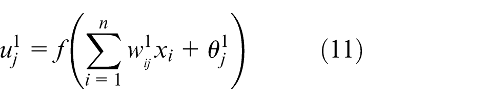
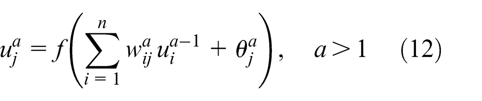
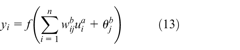
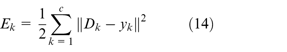
where n denotes the number of neurons in the previous layer, and x_i indicates the neurons in the input layer. a is the number of the hidden layer. f is the activation function that restricts the amplitude of the output of a neuron. The tangential sigmoid function was adopted as an activation function in this study. $w_{ij}^{a}$ indicates the weight that links from a neuron i in the previous layer to a neuron j in the ath layer; and b is the number of neurons in the last hidden layer. $θ_{j}^{a}$ is the bias, which may be used to selectively deter the activity of certain neurons.³²

There are many algorithms that train the NNs. In this study, we adopt the error back-propagation (EBP) algorithm proposed by Rumelhart et al.³³ The EBP algorithm defines the mean squared difference between the real output and the desired output. For example, taking the kth neuron in the output layer yields the mean squared difference as follows

E_{k} = \frac{1}{2} \sum_{k = 1}^{c} ‖ D_{k} - y_{k} ‖^{2}

(14)

where c denotes the number of neurons in the output layer. D_k and y_k are, respectively, the desired and actual outputs of neuron k. For multilayer NNs, training is conducted by continuously renewing weights. The weights can be updated by minimizing the mean squared difference as follows

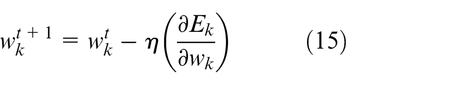
w_{k}^{t + 1} = w_{k}^{t} - η (\frac{\partial E_{k}}{\partial w_{k}})

(15)

where t denotes the learning cycle, and η is termed the learning rates of weights. The computational procedure for updating the weights is explained in detail in Cao et al.³¹

Optimal network architecture

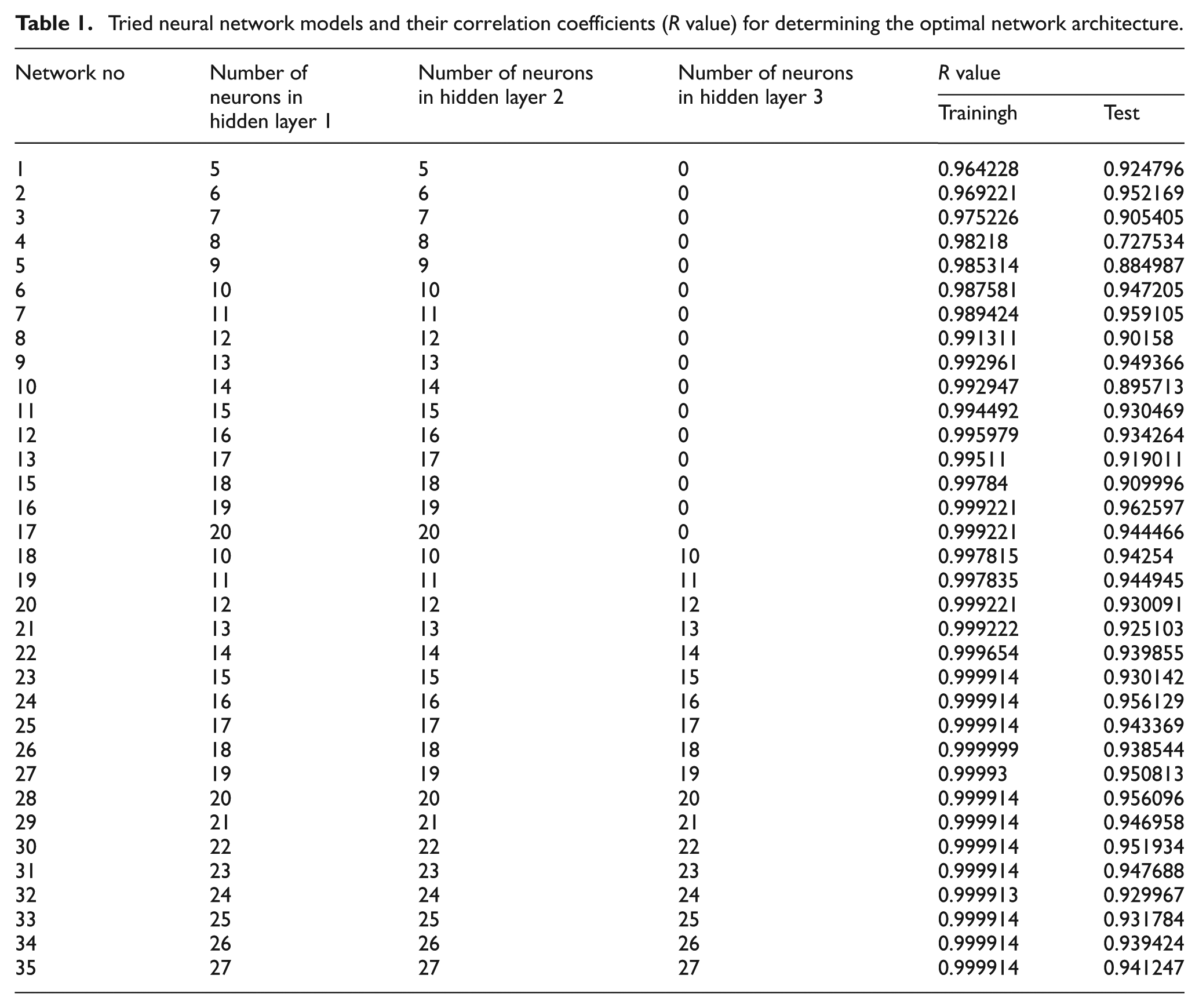
Since the output depends on the number of hidden layers and neurons within it, we should determine the optimal network architecture, that is, the number of hidden layers and neurons within it. In this study, we adopted a trial-and-error approach and thus checked the performance of the NN by trying different numbers of hidden layers and neurons. We checked the correction coefficient (R value) of the performance of each network. The best performance of the network architecture was determined by identifying the maximum correction coefficient.

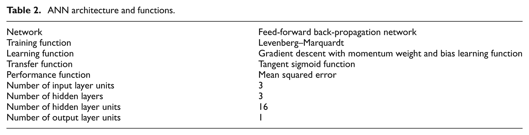
We selected the number of hidden neurons by adopting Bagheripoor and Bisadi’s⁷ approach that determines the number of hidden neurons by minimizing root mean square error (RMSE). Table 1 describes the variation of R values for different trials. The R value was highest when 3 hidden layers and 16 neurons were used. Hence, the NN adopted in this study has 3 hidden layers and 16 neurons. The Levenberg–Marquardt back-propagation learning algorithm was employed to train the NN since it is the fastest method to train a moderate-sized feed-forward NN.³⁴ The NN architecture and functions that were finally determined are summarized in Table 2. In this study, a program of NN has been coded using C-language and implemented.

Table 1.

Tried neural network models and their correlation coefficients (R value) for determining the optimal network architecture.

Network no	Number of neurons in hidden layer 1	Number of neurons in hidden layer 2	Number of neurons in hidden layer 3	R value
Network no	Number of neurons in hidden layer 1	Number of neurons in hidden layer 2	Number of neurons in hidden layer 3	Trainingh	Test
1	5	5	0	0.964228	0.924796
2	6	6	0	0.969221	0.952169
3	7	7	0	0.975226	0.905405
4	8	8	0	0.98218	0.727534
5	9	9	0	0.985314	0.884987
6	10	10	0	0.987581	0.947205
7	11	11	0	0.989424	0.959105
8	12	12	0	0.991311	0.90158
9	13	13	0	0.992961	0.949366
10	14	14	0	0.992947	0.895713
11	15	15	0	0.994492	0.930469
12	16	16	0	0.995979	0.934264
13	17	17	0	0.99511	0.919011
15	18	18	0	0.99784	0.909996
16	19	19	0	0.999221	0.962597
17	20	20	0	0.999221	0.944466
18	10	10	10	0.997815	0.94254
19	11	11	11	0.997835	0.944945
20	12	12	12	0.999221	0.930091
21	13	13	13	0.999222	0.925103
22	14	14	14	0.999654	0.939855
23	15	15	15	0.999914	0.930142
24	16	16	16	0.999914	0.956129
25	17	17	17	0.999914	0.943369
26	18	18	18	0.999999	0.938544
27	19	19	19	0.99993	0.950813
28	20	20	20	0.999914	0.956096
29	21	21	21	0.999914	0.946958
30	22	22	22	0.999914	0.951934
31	23	23	23	0.999914	0.947688
32	24	24	24	0.999913	0.929967
33	25	25	25	0.999914	0.931784
34	26	26	26	0.999914	0.939424
35	27	27	27	0.999914	0.941247

Table 2.

ANN architecture and functions.

Network	Feed-forward back-propagation network
Training function	Levenberg–Marquardt
Learning function	Gradient descent with momentum weight and bias learning function
Transfer function	Tangent sigmoid function
Performance function	Mean squared error
Number of input layer units	3
Number of hidden layers	3
Number of hidden layer units	16
Number of output layer units	1

It should be mentioned that the material used in this study is plain carbon steel (0.15 wt% C, 1.35 wt% Mn, 0.4 wt% Si, and 0.03 wt%) and the model (combination of NN and FEB) has been optimized for the plain carbon steel. However, if a specific material is given, one can still optimize the model by constructing the constitutive relation of the specific material and checking the performance of the NN by trying different numbers of hidden layers and neurons.

Determination of speed difference that minimizes FEB for an arbitrary reduction ratio and material thickness

The NN was trained initially so that FEB was predicted as a function of the reduction ratio for a set of material thicknesses and speed differences. The advantage of training the NN in this manner is that verification of the trained NN is simple. However, an NN trained in this manner cannot promptly determine the speed difference value that minimizes FEB. It should be mentioned that operators in an actual plate rolling mill prefer manipulating the speed difference since FEB on the rolling line can be easily rectified, by means of instant handling of the rotational rates of the lower and upper work roll.

Hence, we replaced the relation between FEB and the reduction ratio for a given material thickness and speed difference, with the relation between FEB and the speed difference for a specific material thickness and reduction ratio. We then coupled the trained NN with the bisection algorithm, which is an incremental search method in which the interval (where the function changes sign) is always divided in half. Figure 7 shows a flow chart to determine the speed difference value that minimizes FEB for an arbitrary reduction ratio and material thickness.

Figure 7.

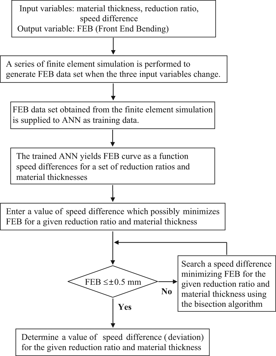
A flow chart to determine a value of speed difference that minimizes FEB whenever a value of reduction ratio and material thickness is provided. Speed difference is defined as the circumferential speed deviation between the top and bottom work rolls.

Results and discussion

Verification of FE model

Before FE analysis is performed to produce the FEB data set, the FE model of plate rolling was verified by comparing the roll forces measured from the pilot hot plate rolling test with those computed from the FE analysis. In Figure 8, the measurements are compared with the predictions for different reduction ratios (22% and 31%), speed differences (0% and 3%), and material thicknesses (25 and 35 mm). The number in the circle indicates the values of the reduction ratio and speed difference, when the material thickness is 25 mm (Figure 8(a)) and 35 mm (Figure 8(b)). Overall, the predictions are in agreement with the measurements. The error between the measurements and the predictions ranges from −6.7% to 7.8%. Thus, the FE model employed in this study has been proven valid and can be used to generate the FEB data set to be used for training the NN.

Figure 8.

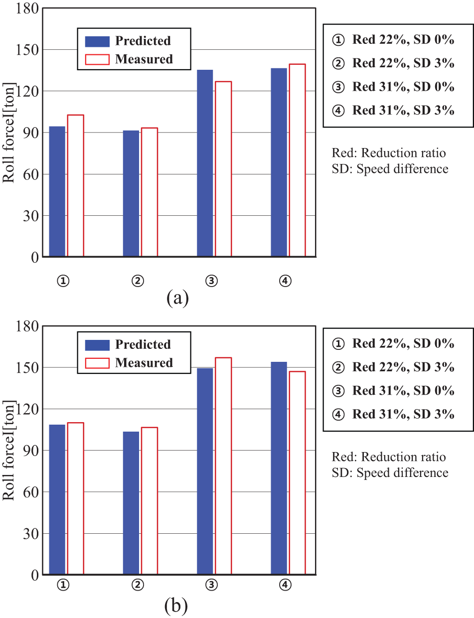
Comparison of the measured roll forces and roll forces predicted by finite element analysis: (a) material thickness is 25 mm and (b) material thickness is 35 mm.

FEB predicted by the trained NN

The trained NN was used to predict the FEB for arbitrary reduction ratios. The FEB behavior can also be plotted as a function of the shape factor (defined as the ratio of mean contact length to mean thickness of material). The variation pattern of FEB behavior as a function of shape factor is similar to that expressed as a function of the reduction ratio. However, using the reduction ratio gives us a more definite physical meaning. Hence, the reduction ratio has been used in this study, instead of the shape factor. Figure 9 shows the FEB behavior of the rolled material plotted as a function of the reduction ratio at a given speed difference and material thickness. The empty symbols indicate the value of FEB obtained from FE simulation. The dashed lines denote the value of FEB predicted by the trained NN.

Figure 9.

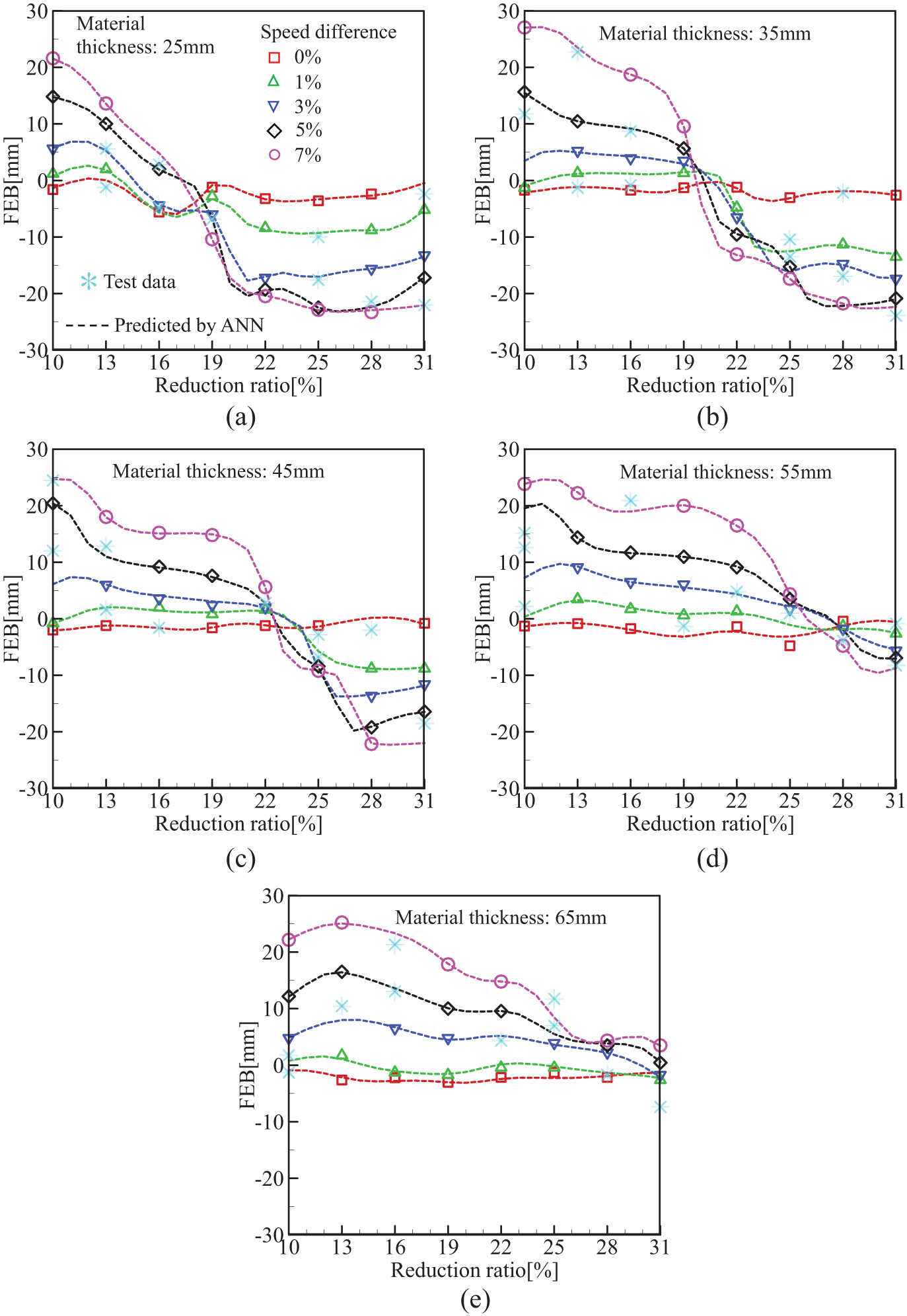
FEB predicted by finite element analysis is marked with symbols. Trained NN yields FEB (marked with dashed line) as a function of reduction ratio for a set of specified material thicknesses and speed differences.

The FEB is positive when the front end of the rolled material bends toward the upper work roll; and it is negative when the front end of the rolled material bends toward the lower work roll. The “∗” symbols in Figure 9(a)–(e) indicate the test data set, which was not used for training the NN. We validated the performance of the trained NN by calculating the RMSE and correction coefficient (R value). A low RMSE (3.0) and high correction coefficient (0.956129) were achieved for the test data sets even though 150 training data set was used for training the NN. Therefore, the trained NN has a good predictive capability. In this light, the trained NN is proven suitable for predicting the FEB behavior when rolling parameters such as reduction ratio, speed difference, and material thickness vary in an arbitrary manner.

We observe that when the speed difference is 0%, the FEB is negative regardless of changes in the reduction ratio. This might be attributable to the setting of the pass-line (or pick-up), which is the distance between the upper vertex of the lower work roll and the underneath of the material entering into the work rolls (Figure 4). In this study, the pass-line was fixed at 20 mm. When the reduction ratio is small, the front end of the rolled material bends toward the upper work roll. However, as the reduction ratio increases, the front end begins to turn downward. We observe that there is a point where the bending behavior, that is, the value of FEB, changes its sign. It is called the neutral point. It occurs when the material is deformed between work rolls whose peripheral speeds are different, and whose reduction ratio per pass (or shape factor) changes. The neutral point moves to higher values of the reduction ratio with increasing material thicknesses. These types of FEB behavior of the rolled material were reported by Philipp et al.² However, the FEB behaviors shown in Figure 9 are slightly different from those reported by Philipp et al.² since Philipp et al. did not consider heat flow between the material and the work roll and set the material temperature as constant (1000 °C) during rolling.

Speed difference minimizing FEB for an arbitrary reduction ratio and material thickness

We cannot determine the speed difference by minimizing FEB from the FEB curve (Figure 9) because FEB curve in Figure 9 was expressed as a function of the reduction ratio for a set of specified material thicknesses and speed differences. Hence, to more precisely determine the speed difference, we transformed the FEB curve so that it was expressed as a function of the speed difference for a set of specified reduction ratios and material thicknesses. The transformed FEB curve could be obtained by extracting the FEB curve (Figure 9) along the ordinate at the selected reduction ratio and material thickness. This procedure is repeated for different reduction ratios and material thicknesses.

Figure 10(a) shows an example of the FEB curve explicitly expressed as a function of the speed difference for the selected reduction ratios (11% and 17%) and material thicknesses (30 and 40 mm). Selection of these reduction ratios and material thicknesses depends on the plate rolling test conditions because the plate rolling test will be performed to verify whether the speed differences determined at the reduction ratios (11% and 17%) and material thicknesses (30 and 40 mm) minimize FEB.

Figure 10.

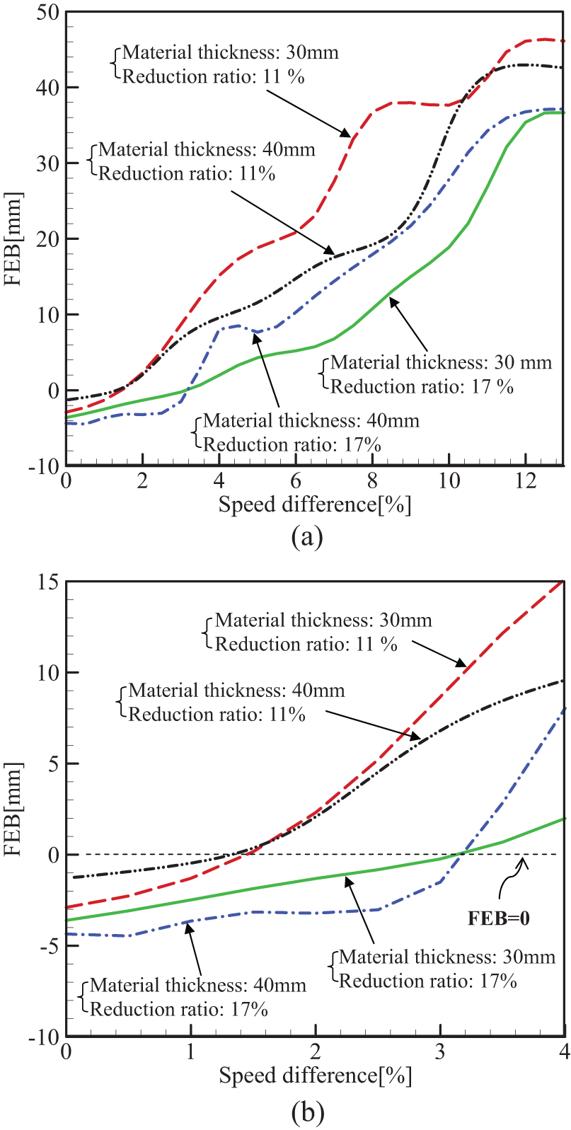
(a) FEB is expressed as a function of the speed difference for two specified reduction ratios and material thicknesses. (b) A range of speed differences is enlarged to see clearly the FEB behavior.

In Figure 10(b), the FEB curve around zero FEB is enlarged so that we can observe the FEB behavior in more detail. Zero FEB denotes that the material front end is perfectly straight along its length direction. The bisection algorithm coupled with the trained NN predicted a set of speed differences that minimized FEB whenever values of reduction ratio and material thickness were entered. Figure 10(b) shows that the speed difference is 1.35% for a material thickness of 40 mm and reduction ratio of 11%; and the speed difference is 1.44% for a material thickness of 30 mm and reduction ratio of 11%. This indicates that the speed difference that minimizes FEB is not affected by the variation in material thickness. Similarly, when a reduction ratio is 17%, the speed difference that minimizes FEB is 3.12% and 3.17% for material thicknesses of 30 and 40 mm, respectively. It is deduced that the reduction ratio considerably affects the speed difference that minimizes FEB.

Applications to a pilot plate rolling mill

A pilot plate rolling test was conducted to verify whether FEB of the rolled material (specimen) is minimized if the speed differences (1.35% and 1.44%; 3.12% and 3.17%) determined for the selected reduction ratios (11% and 17%) and material thicknesses (30 and 40 mm) are applied to the pilot plate rolling mill. In Figure 11, the measured profiles of the rolled material are compared with the profiles of the material with zero FEB. Rectangles marked with a dotted line indicate the profiles of the material with zero FEB, that is, the perfectly flat material (specimen). These profiles are in good agreement, except for Figure 11(b). The measured FEB is bent upward to about 5 mm. Note that the operators in an actual plate mill usually use a nondimensional ratio, the FEB/roll diameter to evaluate the permissible magnitude of FEB.¹⁰ In this light, 5 mm of FEB is a rather low value since the ratio of FEB to the roll diameter in the pilot plate rolling mill is 0.0071 (5/700 mm). This value (0.0071) is much lower than 0.02, which is the ratio allowable in an actual plate rolling mill¹¹ when the material front bends upward along the material length. Therefore, 5 mm of FEB is an acceptable error.

Figure 11.

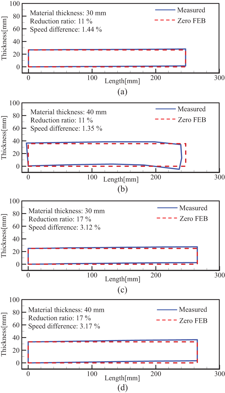
Profiles of the rolled material (specimen) are compared with those of the material with zero FEB. Rectangles marked with a dotted line indicate the profiles of material with zero FEB, that is, the perfectly flat material.

Figure 11(b) shows that the material front end gets bent downward, even though zero FEB is expected. This could be attributed to an experimental error. During the rolling test, metallic oxides were generated on the material surface, but these were manually removed using a thick metal stick. Improper removal of metallic oxides may be one of the uncertainties that lead to unexpected test results since the friction coefficient on the material is affected by metallic oxides on the material surface during the rolling test.

Concluding remarks

This article presents a method to quickly determine the peripheral speed difference on the top and bottom work rolls, which minimizes FEB of a material by coupling a trained NN with the bisection algorithm. We conducted a series of FE simulations of plate rolling and generated an FEB data set by changing the reduction ratio, peripheral speed difference, and entry material thickness. The data set produced from the FE simulation was used to train the NN. Using the proposed method, we then determined the peripheral speed difference that minimizes FEB for an arbitrary value of reduction ratio and entry material thickness. The pilot hot plate rolling test was carried out to confirm the calculation results. Our conclusions are as follows.

The proposed method could quickly predict the peripheral speed difference that minimizes FEB once a value of reduction ratio and entry material thickness was given. The peripheral speed difference predicted by the proposed method could minimize FEB within a margin of maximum error of 5 mm. This error value is rather low since the ratio of FEB to roll diameter in the pilot plate rolling mill is 0.0071 (5/700 mm), which is much lower than the ratio (0.02) in an actual plate rolling mill.¹¹ Therefore, if we can measure the magnitude of material FEB during rolling, the proposed method can be applied to an actual plate mill for in-line control of FEB.

Footnotes

Declaration of conflicting interests

The authors declare that there is no conflict of interest.

Funding

This research received no specific grant from any funding agency in the public, commercial, or not-for-profit sectors.

References

Harrer

Schwenzfeier

. Analysis of the bending of the rolling material in asymmetrical sheet rolling. Int J Mech Sci 2000; 42: 49–61.

Philipp

Schwenzfeier

Fischer

. Front end bending in plate rolling influenced by circumferential speed mismatch and geometry. J Mater Process Tech 2007; 184: 224–232.

Nilsson

. Front-end bending in plate rolling. Scand J Metall 2007; 30: 337–344.

Byon

Lee

. A study to determine a distinct value of front end bending for a given shape factor in flat rolling. Proc IMechE, Part B: J Engineering Manufacture 2011; 225: 2303–2308.

Chun

Moon

. Application of neural networks to predict the width variation in a plate mill. J Mater Process Tech 2001; 11: 146–149.

Korczak

Dyja

Labuda

. Using neural network models for predicting mechanical properties after hot plate rolling processes. J Mater Process Tech 1998; 80: 481–486.

Bagheripoor

Bisadi

. Application of artificial neural networks for the prediction of roll force and roll torque in hot strip rolling process. Appl Math Model 2012; 37: 4593–4607.

Rath

Singh

Bhaskar

. Artificial neural network modelling for prediction of roll force during plate rolling process. Mater Manuf Process 2010; 2: 149–153.

Gudur

Dixit

. A neural network-assisted finite element analysis of cold flat rolling. Eng Appl Artif Intel 2008; 21: 43–52.

10.

Chen

Cheng

. Application of back-propagation neural network for controlling the front end bending phenomenon in plate rolling. Int J Mater Prod Tec 2013; 46: 166–176.

11.

Lee

Park

. Prediction of front end bending in plate rolling process using neural network algorithm. Internal Technical Report, R&D Center, Dangjin, Korea, Hyundai-Steel Company, 2012.

12.

Burden

Faires

. Numerical methods. 4th ed. Boston, MA: Cengage Learning, 1998, pp.33–35.

13.

Jeswiet

Greene

. Experimental measurement of curl in rolling. J Mater Process Tech 1998; 85: 202–209.

14.

Reddy

. An introduction to the finite element method. 2nd ed. London: McGraw-Hill, 1993.

15.

Cook

. Finite element modeling for stress analysis. New York: John Wiley & Sons, 1995.

16.

Hughes

TJR

. The finite element method: linear static and dynamic finite element analysis. New York: Dover Publications, 2000.

17.

ABAQUS version 6.11 documentation. Providence, RI: Dassault Systemes Simulia Corp., 2011.

18.

Alejandro

. Non-linear finite element method simulation and modeling of the cold and hot rolling process. MS Thesis, Virginia Polytechnic Institute and State University, Blacksburg, VA, 2007.

19.

Sun

Yun

Chung

. Investigation of thermomechanical behavior of a work roll and roll life in hot strip rolling. Metall Mater Trans A 1998; 29: 2407–2424.

20.

Lenard

Malinowski

Pietrzyk

. Comparison of the predictive capabilities of mathematical models of the flat rolling process. J Mater Process Tech 1992; 34: 85–92.

21.

Sonboli

Serajzadeh

. Prediction of thermal stresses and temperature field in work rolls during hot strip rolling process. Mater Sci Tech 2010; 26: 343–351.

22.

Dyja

Korczak

. The thermal-mechanical and microstructural model for the FEM simulation of hot plate rolling. J Mater Process Tech 1999; 92–93: 463–467.

23.

Wilson

WRD

Chang

. Interface temperatures in cold rolling. J Mater Shap Technol 1989; 6: 229–240.

24.

Chang

. An efficient way of calculating temperatures in the strip rolling process. J Manuf Sci Eng 1998; 120: 93–100.

25.

Hatta

Kokado

Nishimura

. Analysis of slab temperature change and rolling mill line length in quasi continuous hot strip mill equipped with two roughing mills and six finishing mills. J Jpn Soc Tech Plast 1980; 21: 270–277.

26.

Legrand

Labbe

Weisz-Patrault

. Analysis of roll gap heat transfers in hot steel strip rolling through roll temperature sensors and heat transfer models. Key Eng Mat 2012; 504–506: 1043–1048.

27.

Moon

Lee

. Thermal stress evolution of the roll during rolling and idling in hot strip rolling process. J Therm Stresses 2014; 37: 981–1001.

28.

Chen

Kobayashi

. Rigid-plastic finite element analysis of ring compression, application of numerical methods to forming processes. Appl Mech Div ASME 1978; 28: 163–174.

29.

Devadas

Baragar

Ruddle

. The thermal and metallurgical state of steel strip during hot rolling: part II factors influencing rolling loads. Metall Mater Trans A 1991; 22: 321–333.

30.

Shida

. Empirical formula of flow stress of carbon steels—resistance to deformation of carbon steels at elevated temperature. J Jpn Soc Tech Plast 1969; 10: 610–617 (in Japanese).

31.

Cao

Sugiyamac

Mitsui

. Application of artificial neural networks to load identification. Comput Struct 1998; 69: 63–78.

32.

Schalkoff

. Artificial neural network. Singapore: The McGraw-Hill Companies, Inc., 1997.

33.

Rumelhart

Hinton

Williams

. Learning internal representation by error propagation. Nature 1986; 323: 533–536.

34.

Hagan

Menhaj

. Training feedforward networks with the Marquardt algorithm. IEEE T Neural Networ 1994; 5: 989–993.