
Abstract
This article presents a topological technique for evaluating the performance of a hybrid flow-shop production system. Such a production system is modeled as a hybrid production network; each workstation of the hybrid production network has stochastic capacity levels. This article evaluates the probability of demand satisfaction as a performance indicator for the hybrid production network, in which the network has multiple lines and each workstation has a distinct defect rate. First, a topological transformation is utilized to transform a hybrid flow-shop production system into a network-structured hybrid production network; then, the hybrid production network is decomposed into several routes for flow analysis. Second, two procedures for two models (Model I considers the hybrid production network with parallel lines, Model II with intersectional lines) are designed to generate the minimal required capacity for workstations to satisfy the given demand. The probability of demand satisfaction is subsequently evaluated in terms of the minimal required capacities by applying the recursive sum of disjoint products algorithm.
Keywords
Introduction
In a flow-shop production system, each workstation is made up of several identical machines. Such a production system is a typical hybrid flow-shop production system.1,2 This implies that the workstation has stochastic capacity levels, with performance ranging from a perfectly working order to complete malfunction, due to the failure, partial failure, or maintenance of machines. Hence, the production system also involves stochastic capacity levels, which can be modeled by the capacitated-flow network.3–5 A hybrid flow-shop production system with stochastic capacity levels is termed as a hybrid production network (HPN). In the HPN, arrows represent workstations and nodes represent inspection stations following the workstations. Some studies6,7 have been devoted to constructing a hybrid flow-shop production system as an HPN. Those studies evaluated the demand satisfaction of an HPN on the basis of two assumptions: (1) no flow is increased or decreased during transmission, and (2) no cycle (return) is allowed. Such strong assumptions, however, are not appropriate for an HPN because of the possibility of damage, defect, and rework of products in real life.8–10 In a practical HPN, defective products might be repaired (i.e. rework of defective products) or scrapped.9–11 Therefore, how repair affects the amount of output products is an important issue to consider. More recently, Lin and Chang12,13 proposed an HPN model with only one line to measure the performance of a production network taking single repair into consideration. However, their works lack applicability to multiple lines in most real-life cases.
In order to meet the practical needs of the HPN, this article considers three important characteristics: (1) multiple lines, (2) workstations’ distinct defect rates, and (3) multiple repairs. This article presents a topological technique to transform a production system into a network-structured HPN. The transformed HPN is decomposed into several routes: primary production routes and repair routes. The amount of raw materials and input flow of each workstation can be derived according to the decomposed routes. Subsequently, the minimal required capacity (MRC) is generated for workstations to meet a given demand. The probability of demand satisfaction (PDS) that the HPN could produce d units of product per unit time could be evaluated in terms of MRCs. Two models are considered: Model I considers the HPN with parallel lines, and Model II considers the HPN with intersectional lines, meaning that common workstations process work-in-process (WIP) from different lines. The rest of this article is structured as follows. Two models and assumptions are described in section “Problem statement and assumptions.” The model construction, which uses a topological technique to transform and decompose the HPN, is described in section “Topological model constructions.” Flow analysis and PDS evaluation are formulated in section “Input flow and PDS of HPN.” Two procedures are proposed in section “Procedures for two models” to generate the MRCs for demand in both models. A case-based example of a printed circuit board (PCB) is illustrated in section “Case study of a PCB production system.” The conclusion is summarized in section “Conclusion.”
Problem statement and assumptions
This article measures the performance of the HPN with multiple lines. This article analyzes the input flow of each workstation, where the input flow is the amount of raw materials or WIP each workstation processes per unit time. The PDS is evaluated for a specified demand d as a performance indicator. Two models are considered.
Model I for parallel lines
Two identical lines in parallel produce the same product type. That is, the ordered workstations and their functions in both lines are the same.
Model II for intersectional lines
Two different lines produce the same product type. Most workstations and their functions in both lines are the same. However, one of the two lines may produce a compact product type using fewer workstations. The other line produces more than one product type (regular product type using all workstations and compact product type using fewer workstations). Hence, a common workstation is utilized when producing a regular product type using both lines.
The models to evaluate the PDS of an HPN are developed based on the following assumptions:
All inspection stations (nodes) are perfectly reliable; no WIP or product is damaged by inspection nodes.
The capacity of each workstation (arrow) is a random variable according to a given probability distribution.
The capacities of different workstations (arrows) are statistically independent.
If the defective WIP after repair is still defective, then it is scrapped.
Topological model constructions
A common topological technique is proposed for both models to transform a production system into an HPN. The transformed HPN topology is decomposed into routes for flow analysis.
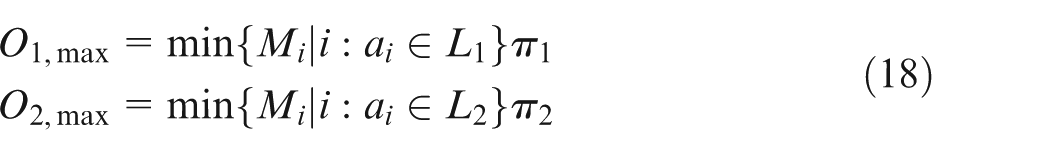
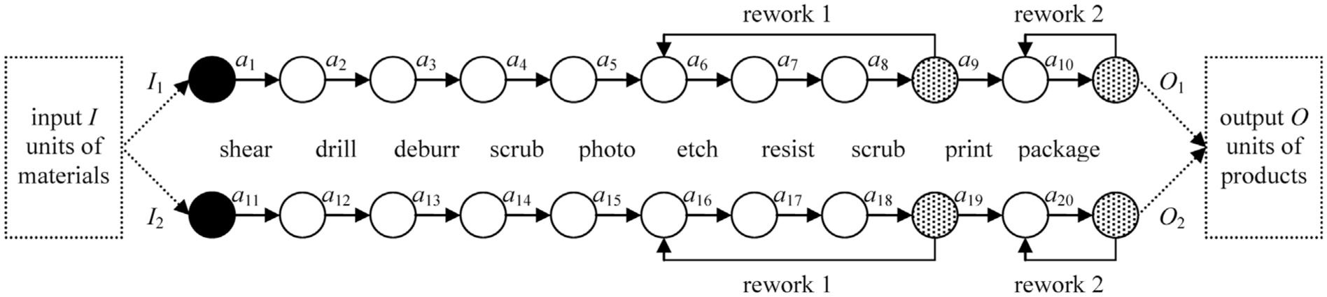
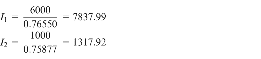
Activity-on-arrow-formed production system
An activity-on-arrow (AOA) diagram is utilized to represent a production system; each arrow denotes a workstation comprising several identical functional machines and each node denotes an inspection station following the workstation. Let (
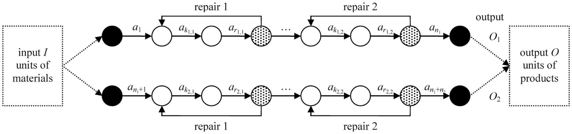
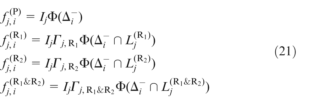
AOA-formed production system in Model I.
Topological technique
The AOA-formed production system is transformed into an HPN to distinguish the input flows from the regular process (without repair) and the repair process. A topological technique is presented to transform the production system into a network-structured HPN. The transformed HPN is shown in Figure 2, in which all the possible routes are depicted in the network topology.
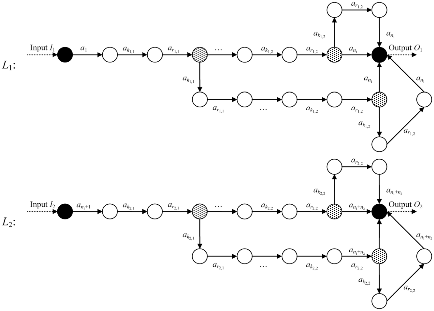
Transformed HPN for Figure 1.
The HPN is further decomposed into routes. Considering that the jth line Lj can make two repairs, there are four combinations for these routes: (1) primary production route
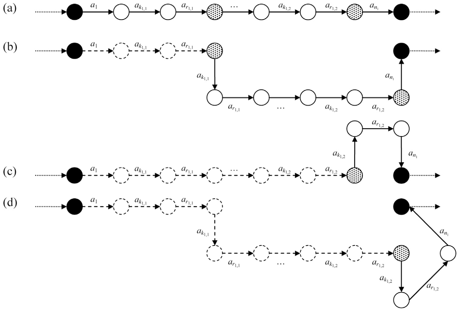
Decomposition for L1 in Figure 2: (a) primary production route without repair, (b) repair route with only the first repair, (c) repair route with only the second repair and (d) repair route with both the first and the second repairs.
Input flow and PDS of HPN
Common formulations are constructed for both models to derive the amount of raw materials and input flow of each workstation. The workload of each workstation and the MRCs for workstations to meet demand are determined according to the amount of raw materials. Thereafter, the PDS of an HPN is calculated in terms of such MRCs.
Amount of raw materials
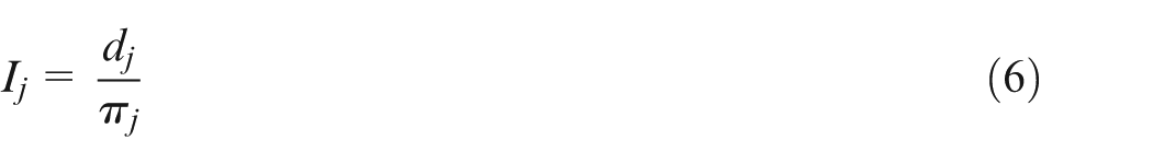
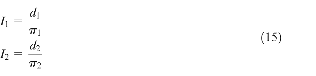
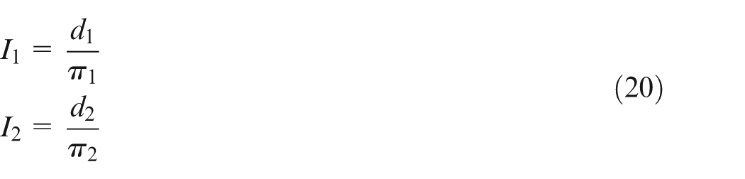
The amount of raw materials should be pre-calculated according to the demand requirement. Because multiple lines are considered in this work, the demand d can be assigned to different lines. For each line Lj, suppose that Ij units of raw materials are able to produce Oj units of product; this article intends to obtain the relationship between Ij and Oj such that Oj satisfies dj and

A set
For instance, given
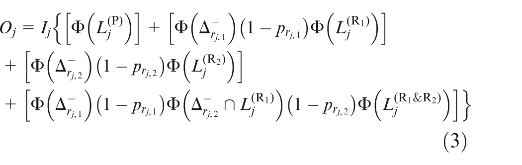
where the first term
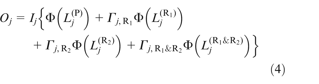
Let

It is necessary that Oj ≥ dj for obtaining sufficient output that satisfies the demand of Lj. The following equation guarantees that the HPN can produce exact sufficient output Oj that satisfies demand dj
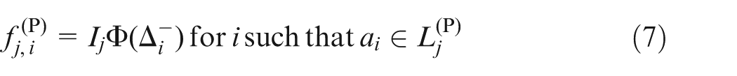
Input flow of each workstation
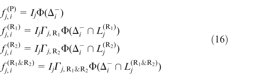
Let
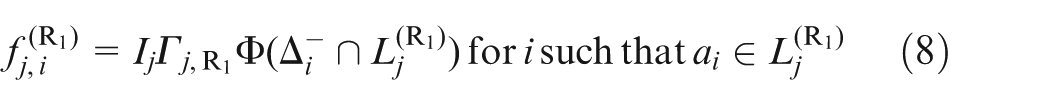
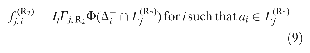
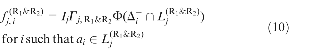
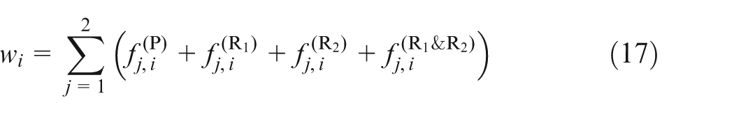
The summation of input flows is defined as the workload of each workstation, denoted by wi. Hence, the workload of ai is
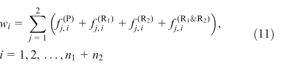
Note that the workload of ai cannot exceed the maximal capacity Mi. If wi > Mi, the PDS is evaluated to be 0.
Let xi denote the capacity of each workstation ai. According to assumption 2, the capacity xi of ai is a random variable, and thus, the HPN is stochastic. Assume that xi takes possible values

PDS
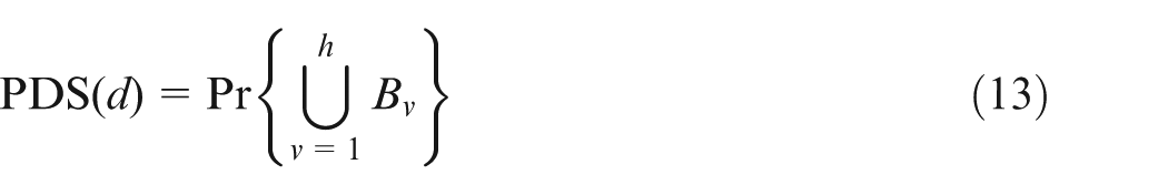
Given the demand d, PDS(d) is the probability that the output product from the HPN is no less than d. Thus, PDS(d) is Pr{X|V(X) ≥ d}, where V(X) is defined as the maximum output under X. That is, all the workstations have to provide sufficient capacities to process the raw materials/WIP and eventually produce enough units of output products. However, it is time-consuming to list all X such that V(X) ≥ d and then sum up their probabilities to derive PDS(d). The minimal ones, say Y, in the set {X|V(X) ≥ d} are claimed to be an MRC for d. Hence, Y is an MRC for d if and only if (1) V(Y) ≥ d and (2) V(X) < d for any capacity state X such that X < Y. Given {Y1, Y2, …, Yh}, the set of MRCs satisfying demand, with the corresponding sets Bv = {X|X ≥ Yv} and v = 1, 2, …, h, the PDS(d) is
Several methods, such as inclusion–exclusion method,6,14,15 disjoint-event method,14,16 state-space decomposition,17–19 and recursive sum of disjoint products (RSDP) algorithm,
20
may be applied to compute
Procedures for two models
Two procedures are presented for both models to generate the MRCs for workstations to satisfy d. The PDS can be derived in terms of MRCs by the RSDP algorithm.
Procedure I: generate MRCs for d in Model I
In Model I, two parallel lines are given, say
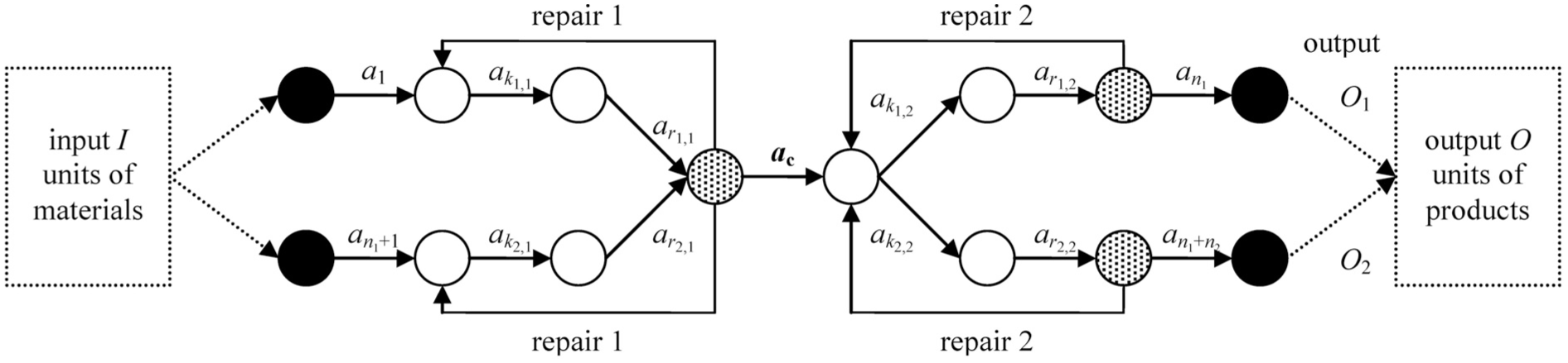
Step 1. Find the maximum output for each route
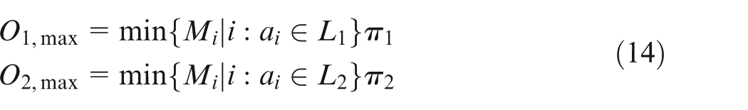
Step 2. Find the demand assignment (d1, d2) satisfying d1 + d2 = d under constraints d1 ≤ O1,max and d2 ≤ O2,max.
Step 3. For each demand pair (d1, d2), do the following steps:
Step 3.1. Determine the amount of input materials for each line by
Step 3.2. Determine the input flows for each workstation ai. For ai∈Lj, the input flows are derived as follows
Step 3.3. Transform input flows from primary production routes and repair routes into workstations’ workload vector
Step 3.4. Find the smallest possible capacity xiα such that xiα ≥ wi > xi(α−1). Then,
Step 4. Those Y obtained in Step 3 are the MRCs for d. Calculate the PDS(d) in terms of MRCs by the RSDP algorithm.
Procedure II: generate MRCs for d in Model II
In Model II, two intersectional lines are given, say L1 = {a1, a2, …,
AOA-formed production system in Model II.
The MRCs for d in Model II are derived with the following steps:
Step 1. Find the maximum output for each route
Step 2. Find the maximum output of the common workstation

If d ≤ Ocmax, go to Step 3; otherwise, stop (i.e. d > Ocmax indicates that the production network cannot satisfy such a demand level).
Step 3. Find the demand assignment (d1, d2) satisfying d1 + d2 = d under constraints d1 ≤ O1,max and d2 ≤ O2,max.
Step 4. For each demand pair (d1, d2), do the following steps:
Step 4.1. Determine the amount of input materials for each line by
Step 4.2. Determine the input flows for each workstation ai. For ai ∈ Lj, the input flows are derived as follows
Step 4.3. Transform input flows from primary production routes and repair routes into workstations’ workload vector
in which the workload of common workstation
Step 4.4. Find the smallest possible capacity xiα such that xiα ≥ wi > xi(α−1). Then,
Step 5. Those Y obtained in Step 4 are the MRCs for d. Calculate the PDS(d) in terms of MRCs by the RSDP algorithm.
Case study of a PCB production system
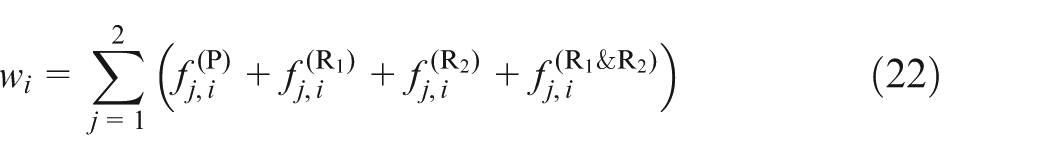
A PCB production system is adopted to illustrate the PDS evaluation for both models. The function, success rate, and capacity data of each workstation are provided in Table 1. The capacity is measured in terms of pieces of boards processed per day (pcs/day). For instance, the specification of a deburring machine is estimated as 300,000 ft2/month. Hence, for the board size of 24″ × 24″, the capacity of the deburring machine is 75,000 pcs/month (i.e. 2500 pcs/day). The deburring workstation a3 comprising four machines has five capacity levels, say {0, 2500, 5000, 7500, 10,000}. 13 The lowest level 0 corresponds to complete malfunction of all machines, while 10,000 is the highest level, at which all machines operate successfully. The capacity distribution is in the form of probability mass function, indicating that each workstation can provide a certain capacity level with a corresponding probability. For instance, the probability that a3 can produce 5000 pcs/day (or more) is Pr{x3≥5 000} = Pr{x3=5000} + Pr{x3 = 7500} + Pr{x3 = 10,000} = 0.003 + 0.015 + 0.980 = 0.998.
Workstation data of PCB production system.
The unit of capacity is processed per day.
For both models, the PCB production system has to satisfy d = 7000 pcs/day, with output boards beingbatched by every 1000 boards. The PDSs for both models are derived in the following subsections.
Model I
In Model I, two identical lines, L1 and L2, are in parallel. The defective WIP outputs from a8 and a18 are repaired starting from a6 and a16, respectively (see Figure 5). The defective product outputs from a10 and a20 can be repaired by the same workstation. The first line L1 is divided into one primary production route
Step 1. Find the maximum output for each route
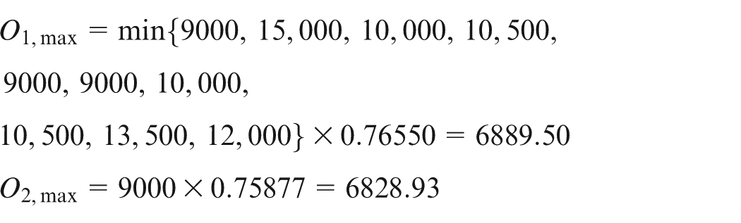
Step 2. Find the demand assignment (d1, d2) satisfying d1 + d2 = 7000 under constraints d1 ≤ 6889.50 and d2 ≤ 6828.93. Since the output boards are batched by every 1000 boards, the feasible demand pairs are D1 = (6000, 1000), D2 = (5000, 2000), D3 = (4000, 3000), D4 = (3000, 4000), D5 = (2000, 5000), and D6 = (1000, 6000).
Step 3. For each demand pair (d1, d2), do the following steps:
(a) For D1 = (6000, 1000)
Step 3.1a. Determine the amount of input materials for each line by

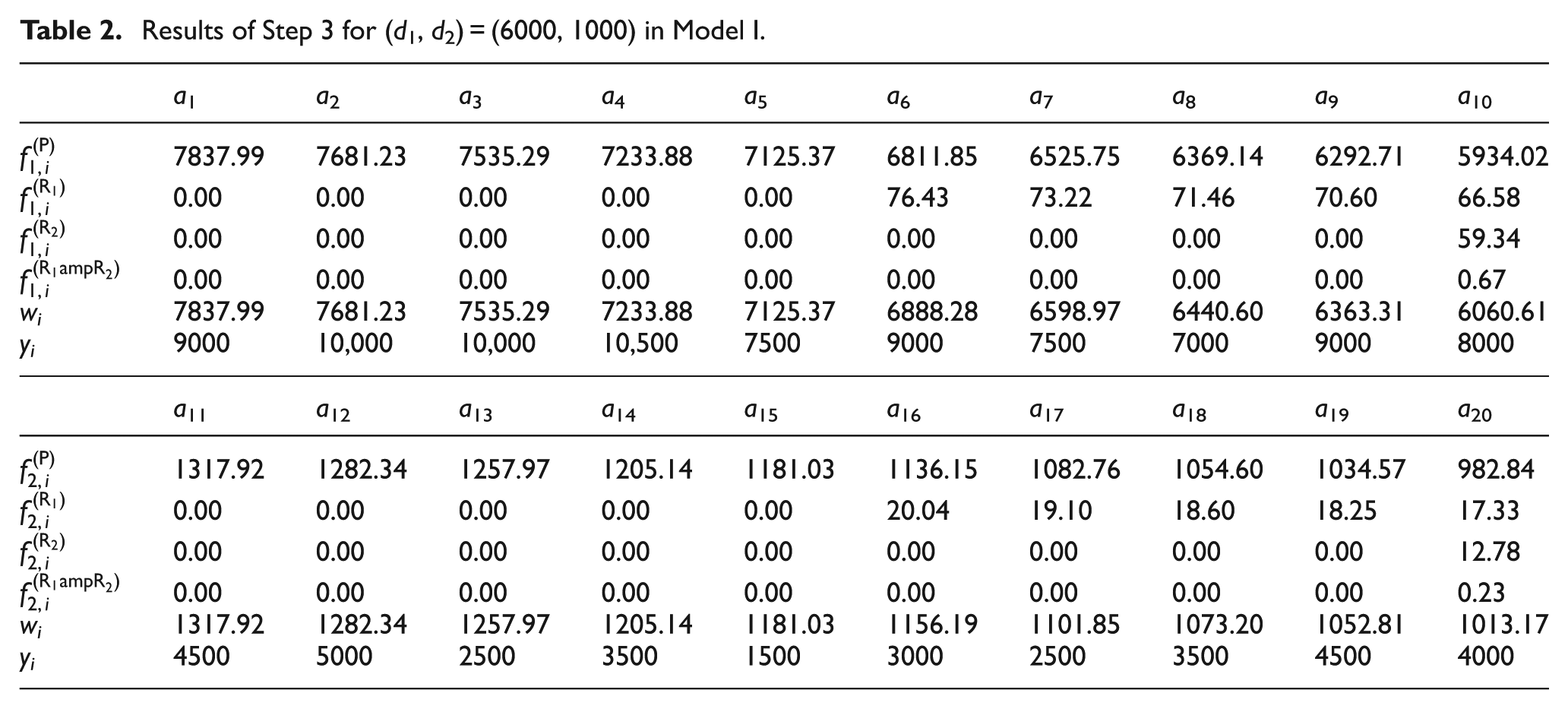
Step 3.2a. For demand pair D1 = (6000, 1000), the input flow of each workstation is shown in Table 2 (see the row of fj, i).
Step 3.3a. Transform input flows from both primary production route and repair route into the workstations’ workload vector W1. The calculation process is summarized in Table 2 (see the row of wi).
Step 3.4a. Calculate the MRC Y1 for pair D1 = (6000, 1000). The calculation process is summarized in Table 2 (see the row of yi).
(b) For D2 = (5000, 2000)
#x022EE;
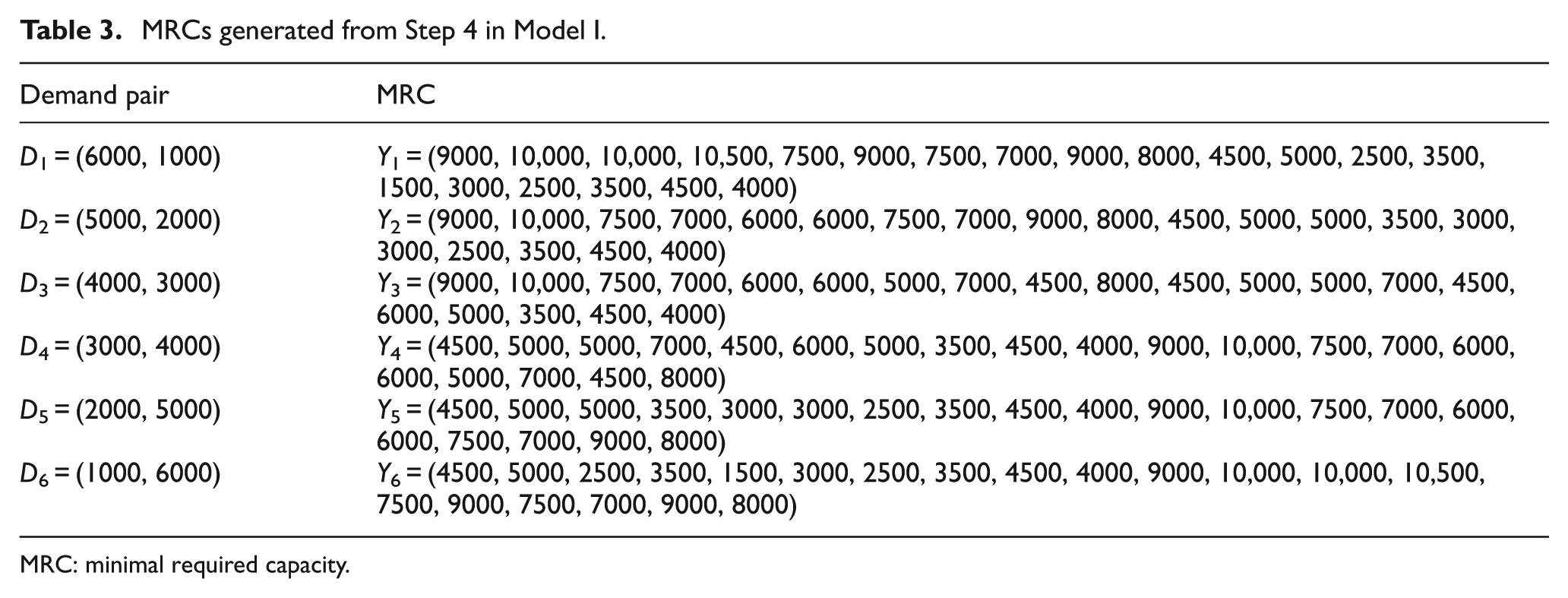
Step 4. Six MRCs for d = 7000 are obtained from Step 3. The results are summarized in Table 3. PDS(7000) = 0.87931 by the RSDP algorithm.
PCB production system in Model I.
Results of Step 3 for (d1, d2) = (6000, 1000) in Model I.
MRCs generated from Step 4 in Model I.
MRC: minimal required capacity.
Model II
In Model II, the drilling workstation
Step 1. Find the maximum output for each route
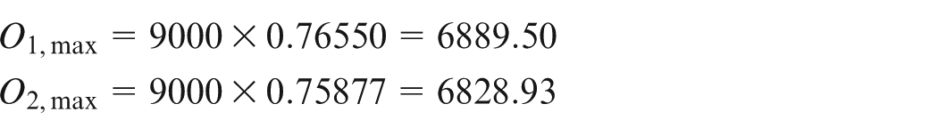
Step 2. Find the maximum output of the common workstation
Step 3. Find the demand assignment (d1, d2) satisfying d1+d2 = 7000 under constraints d1 ≤ 6889.50 and d2 ≤ 6828.93. Since the output boards are batched by every 1000 boards, the feasible demand pairs are D1 = (6000, 1000), D2 = (5000, 2000), D3 = (4000, 3000), D4 = (3000, 4000), D5 = (2000, 5000), and D6 = (1000, 6000).
Step 4. For each demand pair (d1, d2), do the following steps:
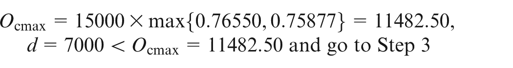
(a) For D1 = (6000, 1000)
Step 4.1a. Determine the amount of input materials for each line by
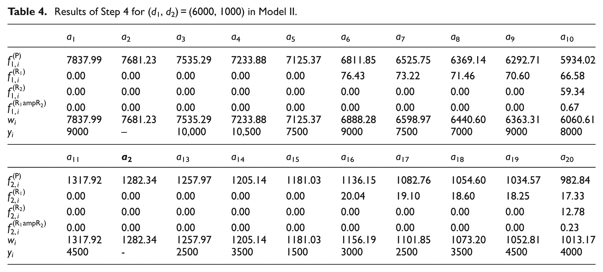
Step 4.2a. For demand pair D1 = (6000, 1000), the input flow of each workstation is shown in Table 4 (see the row of fj, i).
Step 4.3a. Transform input flows from both primary production route and repair route into the workstations’ workload vector W1. Note that the workload of the common workstation
Step 4.4a. Calculate the MRC Y1 for pair D1 = (6000, 1000). The calculation process is summarized in Table 4 (see the row of yi).
(b) For D2 = (5000, 2000)
⋮
Step 5. Six MRCs for d = 7000 are obtained from Step 4. The results are summarized in Table 5. PDS(7000) = 0.86194 is derived by the RSDP algorithm.
PCB production system in Model II.
Results of Step 4 for (d1, d2) = (6000, 1000) in Model II.
MRCs generated from Step 5 in Model II.
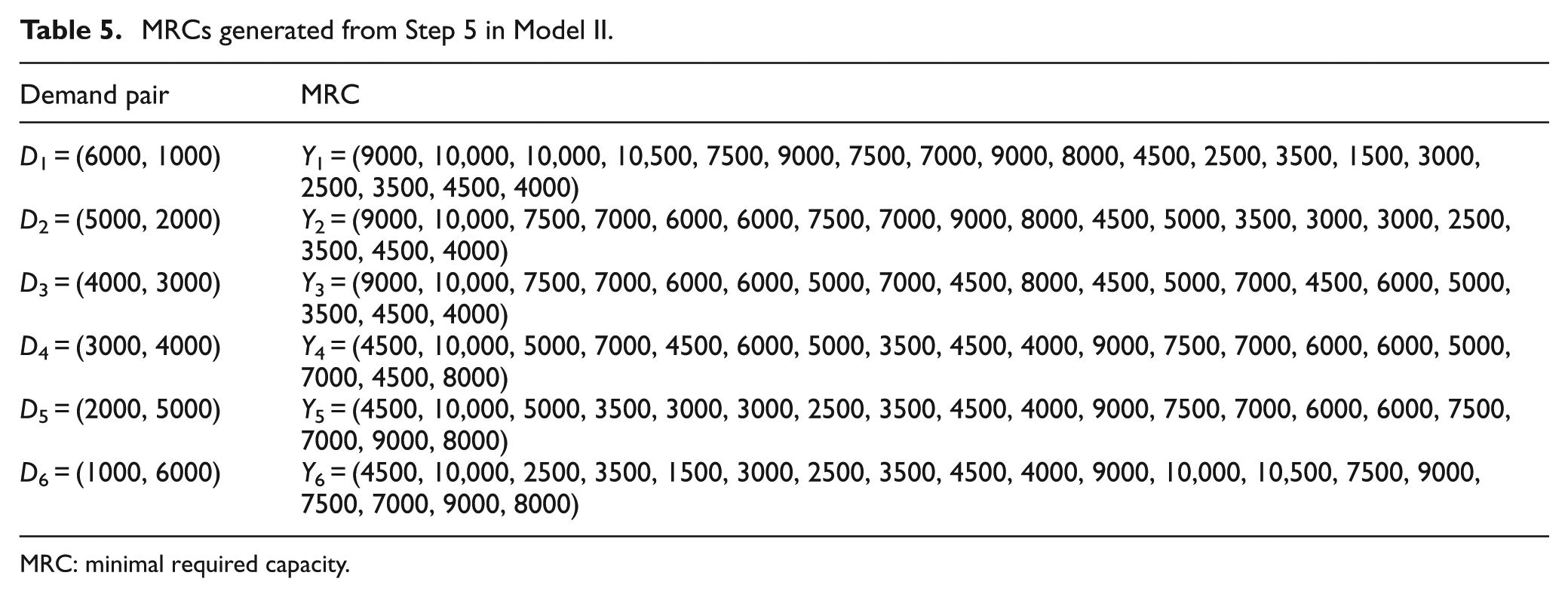
MRC: minimal required capacity.
Conclusion
This article constructs a hybrid flow-shop production system as an HPN using the topological technique to evaluate the PDS. Three practical characteristics are considered: (1) multiple lines, (2) workstations’ distinct defect rates, and (3) multiple repairs. Two models are studied in this article. Model I considers parallel lines producing the same product type; Model II considers intersectional lines with common workstations producing the same product type. Two procedures are developed to generate all MRCs that satisfy demand d for both models. In terms of MRCs, the PDS is derived using the RSDP algorithm.
Future research can be devoted to conducting a sensitivity analysis to investigate which workstation in an HPN is most important for improving the PDS. One possible method of sensitivity analysis is to increase the capacity of one workstation at a time (the others retain the same conditions). Once the capacity of a workstation is increased, the PDS is also improved. Eventually, the production manager can investigate which workstation increases the PDS most, making it the most important one in the HPN.
One more possible issue for future research is to address competence management in an HPN. Competence management can involve a more multidimensional and comprehensive approach.21,22 For instance, experience knowledge management, skills-gap analysis, succession, planning competency analysis, and profiling can be involved in the continuous improvement of competence management. These can be used with the PDS proposed in this article to provide a more comprehensive assessment.
Footnotes
Declaration of conflicting interests
The author(s) declared no potential conflicts of interest with respect to the research, authorship, and/or publication of this article.
Funding
The author(s) disclosed receipt of the following financial support for the research, authorship, and/or publication of this article: This work was supported in part by the Ministry of Science and Technology, Taiwan, ROC, under grant nos MOST 102-2221-E-011-080-MY3 and MOST 103-2218-E-011-010-MY3.