Sage Journals: Discover world-class research

Abstract

This article addresses reliability evaluation for a production system with intersectional lines and multiple reworking actions, where the reliability is the probability of demand satisfaction. First, the production system is constructed as a capacitated-flow production network by the revised graphical transformation and decomposition techniques. Capacity analysis is implemented to determine the input flow of each workstation subsequently. Second, two algorithms, including a general algorithm, are proposed to generate all minimal capacity vectors that workstations should provide to satisfy demand. The reliability is derived in terms of such vectors accordingly. A real-world case of printed circuit board production system is utilized to demonstrate the performance evaluation procedure.

Keywords

Reliability intersectional lines demand satisfaction printed circuit board production system

Introduction

From the perspective of engineering manufacturing, this article addresses the performance evaluation of a production system with intersectional lines. The reliability, which is defined as probability of demand satisfaction, is utilized to assess the performance of the production system. In a production system, each line consists of a sequence of workstations and each workstation has a specific function. Multiple lines are designed to produce products with higher efficiency and flexibility.^1–3 Shared workstation capacity is normal in a production system with multiple lines. One commonly occurring scenario is that a workstation layout in an original line may have much high capacity than others. When a new line is designed, it is possible for the workstation with higher capacity to serve as a common workstation. Hence, the attribute of intersectional lines is taken into account in this article, meaning that common workstation is addressed in the production system.

Network analysis is an applicable approach to represent a production system. The activity-on-arc (AOA) diagram is achievable to model a production system as a network; each arc denotes a workstation of identical machines and each node denotes an inspection station following the workstation. In particular, each workstation in the production network possesses stochastic capacity states due to failure, partial failure, or maintenance. Therefore, the capacity states of a production network are also stochastic, and it can be treated as the so-called capacitated-flow network.^4–6 In this article, we term the production system with stochastic capacities as capacitated-flow production network (CFPN).

Some studies^7–9 have been devoted to reliability evaluation of production system by applying the capacitated-flow network model. Those studies evaluated the reliability of CFPN in terms of minimal paths (MPs), where an MP is a path, which contains no cycle.¹⁰ A great deal of research^4–6,8–11 has been devoted to studying the reliability of a capacitated-flow network in terms of MPs. In those researches, the demand transmitted through a network must obey the flow conservation,¹² implying that no flow will be increased or decreased during transmission. Such a strong assumption is improper for a CFPN because the input flow and output flow of the CFPN are not the same due to the defect of workstation.

Defect of workstation is a critical reliability factor that should be concerned, particularly in a highly automated production system.^13,14 Defective products in a production system might be reworked or scrapped. In several applications, the reworking action is implemented by the same workstations for repairing products. This implies that a production system has two paths, the general production path and the reworking path, to produce products.^15,16 However, based on the MP concept, an arc (workstation) would not appear on the same path more than once; otherwise, it is not an MP. In a practical CFPN, defective work-in-process (WIP) from a workstation may be reworked starting from previous workstation(s) or the same workstation(s),^15,16 which is breaking the basic concept of MP.

To overcome the limitations of flow conservation and MP, Lin et al.³ proposed a graphical methodology to transform the production system into a network-structured CFPN. In particular, this study concentrated on the case of parallel lines, which does not allow common workstations because products are produced by each line independently. Moreover, only one reworking action in each line is considered in the literature.³ For the more practical case of intersectional lines, the previous literature cannot be applied to calculate the capacity that the common workstation should provide because input flows are from different lines. In order to assess the reliability of demand satisfaction for a CFPN with intersectional lines and multiple reworking actions, this article modifies the methodology proposed in the study by Lin et al.³ to deal with the flow and capacity of each common workstation. The reminder of this article is organized in the following. Model building for the CFPN with intersectional lines and multiple reworking actions is constructed in section “Model building.” Flow analysis and reliability evaluation are formulated in section “Flow analysis and reliability.” A case study of printed circuit board (PCB) production system is demonstrated in section “Case study.” Conclusion of this article are summarized in section “Conclusion and future research.”

Model building

The instantaneous production rate in a CFPN is defined as demand, which is measured in d units of products produced per unit time. To analyze the capacity of the CFPN, we emphasize the input flow of each workstation, where the input flow is defined as the input amount of raw materials/WIP that each workstation processes per unit time. For convenience, this article first concentrates on the case of two lines with a common workstation. Subsequently, the proposed techniques and algorithm are extended to the general case of more than two lines. To evaluate the reliability of the CFPN, some assumptions are addressed as follows:

Each inspection station (node) is perfectly reliable.

The capacity of each workstation (arc) is a random variable according to a given probability distribution.

The capacities of different workstations are statistically independent.

Each defective WIP is reworked at most once by the same workstation.

AOA-formed representation

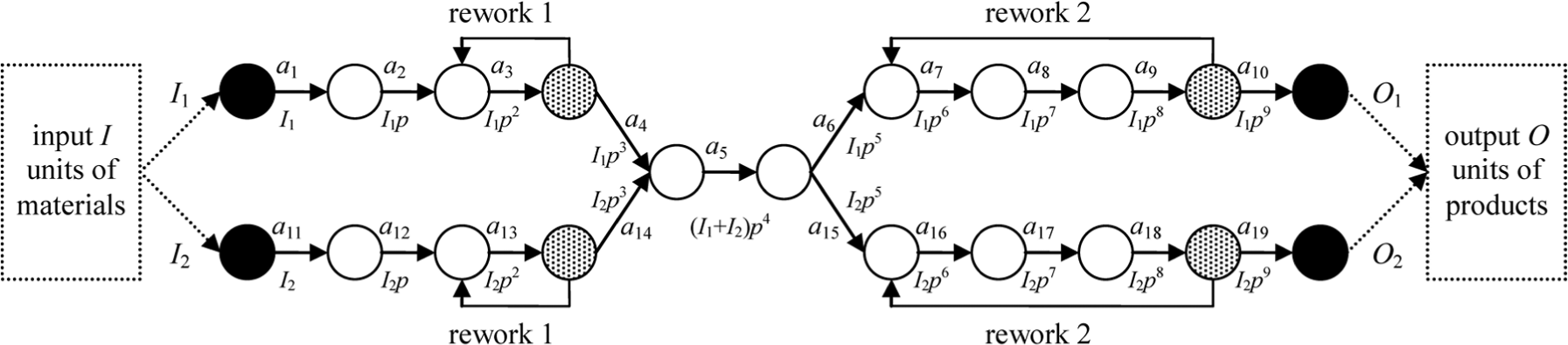
An AOA diagram is adopted to represent a production system with intersectional lines; each arc denotes a workstation consisting of several identical machines, and each node denotes an inspection station following the workstation. Let (N, A) denote a production system with two lines and a common workstation a_c, where N represents the set of nodes and A = {a_i|i = 1, 2, …, n₁+n₂} represents the set of arcs with n₁ and n₂ being the number of workstations in the first line L₁ and the second line L₂, respectively. Figure 1 represents a production system in the form of AOA diagram with L₁ = {a₁, a₂, …, a ₅ , …, a₁₀} and L₂ = {a₁₁, a₁₂, …, a ₅ , …, a₁₉}. Note that a ₅ is a common workstation who shares its capacity and is marked in boldface. Without loss of generality, we assume that a ₅ is layout in L₁ (i.e. n₁ = 10 and n₂ = 9). The success rate of workstation is p, where 0 ≤p≤ 1 (i.e. the defect rate is q = 1 −p).

Figure 1.

A production system in the form of AOA diagram.

In Figure 1, two black nodes in each line represent the input and output inspection stations, respectively. White nodes between two workstations denote the inspection stations for WIP to check whether the WIP can enter the next process or should be scrapped. The meshed nodes indicate that defective WIP inspected by these inspection stations can be reworked. The first reworking action is that defective WIP output from a₃ (resp. a₁₃) is reworked by itself, while the second reworking action is that defective WIP output from a₉ (resp. a₁₈) is reworked starting from a₇ (resp. a₁₆).

Revised transformation and decomposition techniques

The production system in the form of AOA diagram only provides the directions that WIP should enter. It is difficult to represent the amount of input flows from both the regular (without reworking) and the reworking processes by the AOA diagram. To analyze the input flows of each workstation, especially for the common workstation, this article modifies the transformation and decomposition techniques proposed in the study by Lin et al.³ for the case of intersectional lines and multiple reworking actions.

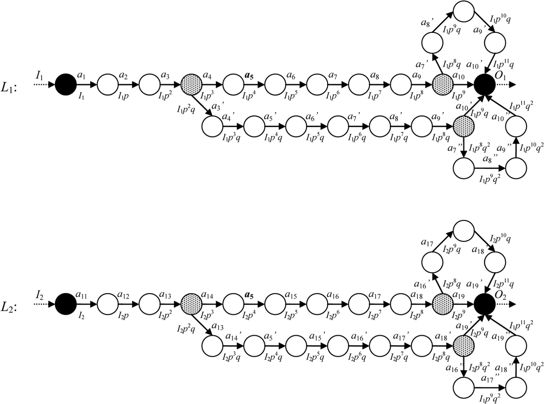
The production system is transformed into a network-structured CFPN, as shown in Figure 2, in which the input amount of workstation is under each arc. In particular, dummy workstations $a'_{i}$ and $a ″_{i}$ are utilized to denote a_i operating the reworking action. In particular, a ₅ appears in both lines because it serves as a common workstation in the CFPN. The transformed CFPN is beneficial for further analysis because it is easy to represent the input amount from regular and reworking processes of each workstation.

Figure 2.

Network-structured CFPN.

To analyze the input flow of workstations, each line L_j is decomposed into several paths. The decomposition technique originally proposed in the study by Lin et al.³ only considered one reworking action. However, while two reworking actions are considered, there are four combinations of paths: (a) production path without reworking action, (b) reworking path with the first reworking action, (c) reworking path with the second reworking action, and (d) reworking path with both the first and second reworking actions. In this article, combination (a) is termed general production path $L_{j}^{(G)}$ ; combinations (b) and (c) are termed single-reworking paths $L_{j}^{(R | r_{1}, r_{1} - k_{1})}$ and $L_{j}^{(R | r_{2}, r_{2} - k_{2})}$ , respectively; combination (d) is termed double-reworking path $L_{j}^{(R | (r_{1}, r_{1} - k_{1}), (r_{2}, r_{2} - k_{2}))}$ .

Take L₁ in Figure 2 for instance, the set {a₁, a₂, a₃, a₄, a ₅ , a₆, a₇, a₈, a₉, a₁₀} is a general production path $L_{1}^{(G)}$ (Figure 3(a)). The single-reworking path with the first reworking action is $L_{j}^{(R | r_{1}, r_{1} - k_{1})} = L_{1}^{(R | 3, 3 - 0)} = L_{1}^{(R | 3, 3)} = {a_{1}, a_{2}, a_{3}, a'_{3}, a'_{4}, a'_{5}, a'_{6}, a'_{7}, a'_{8}, a'_{9}, a'_{10}}$ ; therepresentation (R|3,3–0) indicates that defective WIP output from the third ordered (r₁ = 3) workstation (a₃) is reworked by the original (k₁ = 0) workstation. In fact, no defective WIP is processed by a₁, a₂, and a₃, and the input flow should be 0 for these workstations. Thus, a₁, a₂, and a₃ can be neglected and merely the workstations $a'_{3}, a'_{4}, \dots, a'_{10}$ doing reworking action are retained. Since the workstation a_i and the dummy workstation $a'_{i}$ are the same, the single-reworking path is simplified as $L_{1}^{(R | 3, 3)} = {a_{3}, a_{4}, a_{5}, a_{6}, a_{7}, a_{8}, a_{9}, a_{10}}$ (Figure 3(b)). By the same operations, $L_{1}^{(R | 9, 9 - 2)} = L_{1}^{(R | 9, 7)} = {a_{7}, a_{8}, a_{9}, a_{10}}$ in which (R|9,9–2) indicates that defective WIP output from the ninth ordered (r₂ = 9) workstation (a₉) is reworked by the previous two (k₂ = 2) workstations (a₇) (Figure 3(c)). Finally, the double-reworking path $L_{1}^{(R | (3, 3), (9, 7))} = {a_{7}, a_{8}, a_{9}, a_{10}}$ is obtained (Figure 3(d)). For L₂, we have $L_{2}^{(G)} = {a_{11}, a_{12}, a_{13}, a_{14}, a_{5}, a_{15}, a_{16}, a_{17}, a_{18}, a_{19}}$ , $L_{2}^{(R | 3, 3)} = {a_{13}, a_{14}, a_{5}, a_{15}, a_{16}, a_{17}, a_{18}, a_{19}}$ , $L_{2}^{(R | 9, 7)} = {a_{16}, a_{17}, a_{18}, a_{19}}$ , and $L_{2}^{(R | (3, 3), (9, 7))} = {a_{16}, a_{17}, a_{18}, a_{19}}$ . The following flow analysis of each workstation is based on the decomposed paths.

Figure 3.

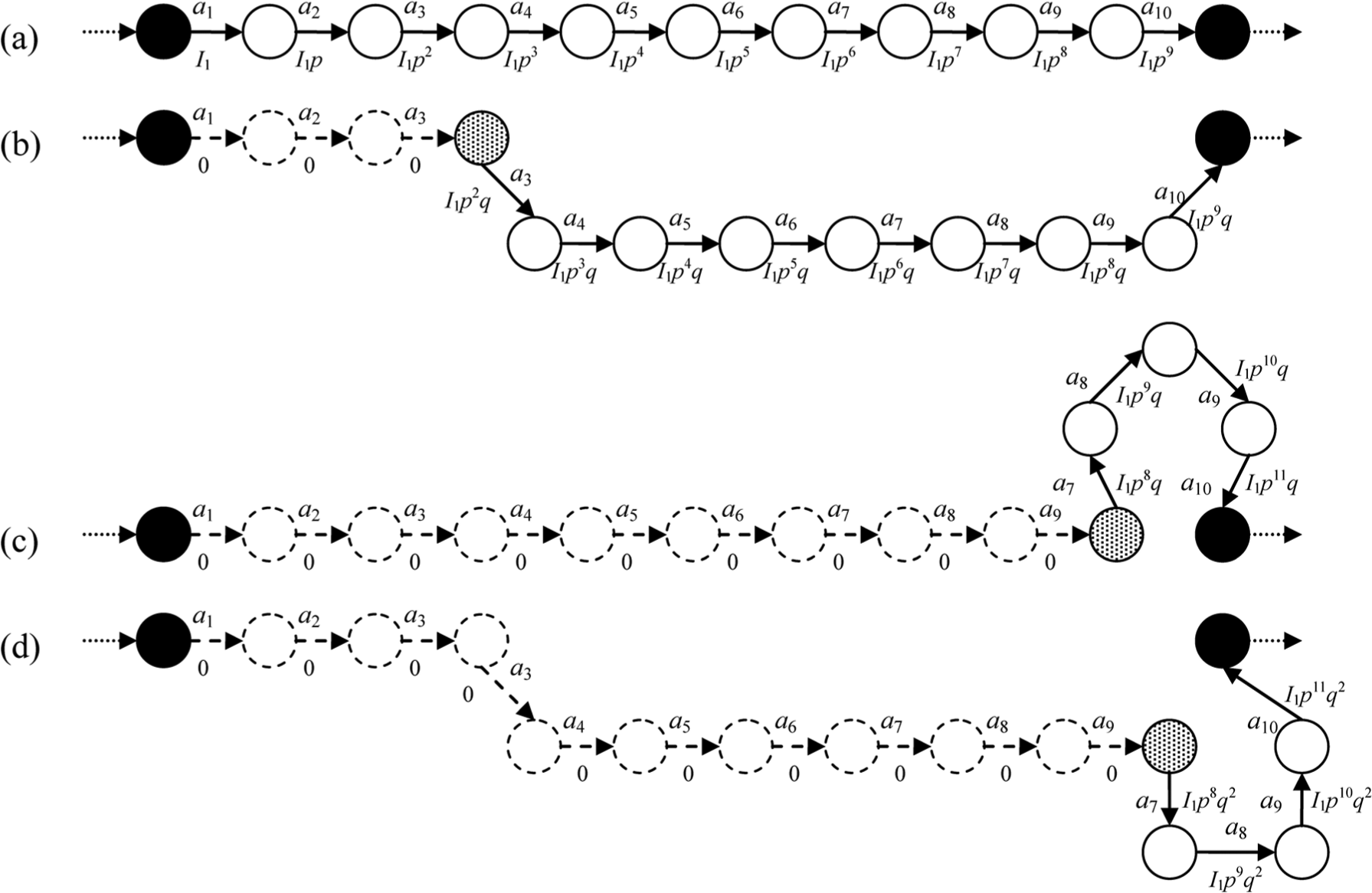
Decomposed paths for L₁. (a) production path without reworking action, (b) reworking path with the first reworking action, (c) reworking path with the second reworking action, and (d) reworking path with both the first and second reworking actions

Flow analysis and reliability

The amount of raw materials should be determined prior to input flow analysis. Then, the input flow of each workstation is calculated in terms of the amount of raw materials. Based on the flow analysis, the reliability is determined to evaluate the demand satisfaction.

Input flow analysis

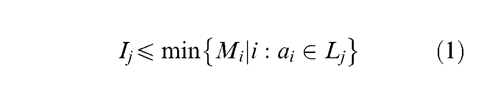
Let d_j be the assigned demand for L_j and d₁+d₂ = d. Suppose that I_j units of raw material are able to produce O_j units of product for L_j; we intend to derive the relationship between I_j and O_j such that O_j satisfies d_j. Note that I_j cannot exceed the maximum capacity M(L_j) of L_j, where M(L_j) = min{M_i|i: a_i∈L_j}. That is, M(L_j) is determined by the bottleneck workstation at line L_j. Hence, we have the following constraint

I_{j} \leq min {M_{i} | i : a_{i} \in L_{j}}

(1)

Let n denote the number of workstations in L_j by taking a_c into account. For instance, in Figure 1, we have n = n₁ = n₂+ 1 = 10 because a ₅ is layout in L₁. Hence, the expected output amount for L_j is

O_{j} = (I_{j} p^{n} + I_{j} p^{n + k_{1}} q + I_{j} p^{n + k_{2}} q + I_{j} p^{n + k_{1} + k_{2}} q^{2})

(2)

where the first term (I_jpⁿ) is produced by $L_{j}^{(G)}$ . The second term ( $I_{j} p^{n + k_{1}} q$ ) and the third term ( $I_{j} p^{n + k_{2}} q$ ) are processed by $L_{j}^{(R | r_{1}, r_{1} - k_{1})}$ and $L_{j}^{(R | r_{2}, r_{2} - k_{2})}$ , respectively. The last term ( $I_{j} p^{n + k_{1} + k_{2}} q^{2}$ ) is processed by $L_{j}^{(R | (r_{1}, r_{1} - k_{1}), (r_{2}, r_{2} - k_{2}))}$ .

It is necessary that O_j≥d_j for obtaining sufficient output that satisfies the assigned demand d_j. Thus, we have the following constrain

I_{j} \geq \frac{d_{j}}{(p^{n} + p^{n + k_{1}} q + p^{n + k_{2}} q + p^{n + k_{1} + k_{2}} q^{2})}

(3)

For convenience, let $η_{j} = (p^{n} + p^{n + k_{1}} q + p^{n + k_{2}} q + p^{n + k_{1} + k_{2}} q^{2})$ , meaning that η_j is the overall success rate of L_j. Equation (4) guarantees the CFPN produces exact output O_j that satisfies assigned demand d_j

I_{j} = \frac{d_{j}}{η_{j}}

(4)

Once the input amount of raw materials is determined, the input flow analysis of each workstation can be derived.

To calculate the input flow of each workstation, we utilize $f_{j, i}^{(G)}$ , $f_{j, i}^{(R | r_{1}, r_{1} - k_{1})}$ , $f_{j, i}^{(R | r_{2}, r_{2} - k_{2})}$ , and $f_{j, i}^{(R | (r_{1}, r_{1} - k_{1}), (r_{2}, r_{2} - k_{2}))}$ to represent the input amount of the ith workstation in the jth line for $L_{j}^{(G)}$ , $L_{j}^{(R | r_{1}, r_{1} - k_{1})}$ , $L_{j}^{(R | r_{2}, r_{2} - k_{2})}$ , and $L_{j}^{(R | (r_{1}, r_{1} - k_{1}), (r_{2}, r_{2} - k_{2}))}$ , respectively. The input flow (raw materials/WIP) processed by a_i should satisfy

f_{j, i}^{(G)} + f_{j, i}^{(R | r_{1}, r_{1} - k_{1})} + f_{j, i}^{(R | r_{2}, r_{2} - k_{2})} + f_{j, i}^{(R | (r_{1}, r_{1} - k_{1}), (r_{2}, r_{2} - k_{2}))} \leq M_{i} for i such that a_{i} \in L_{j}

(5)

Constraint (5) indicates that the total amount of input flow entering a_i does not exceed the maximal capacity M_i. The term $(f_{j, i}^{(G)} + f_{j, i}^{(R | r_{1}, r_{1} - k_{1})} + f_{j, i}^{(R | r_{2}, r_{2} - k_{2})} + f_{j, i}^{(R | (r_{1}, r_{1} - k_{1}), (r_{2}, r_{2} - k_{2}))})$ is defined as the loading w_i of a_i. The following equation determines the loading of a_i

w_{i} = f_{j, i}^{(G)} + f_{j, i}^{(R | r_{1}, r_{1} - k_{1})} + f_{j, i}^{(R | r_{2}, r_{2} - k_{2})} + f_{j, i}^{(R | (r_{1}, r_{1} - k_{1}), (r_{2}, r_{2} - k_{2}))} for i such that a_{i} \in L_{j}

(6)

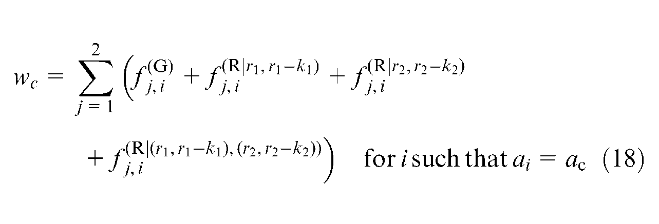
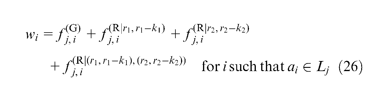
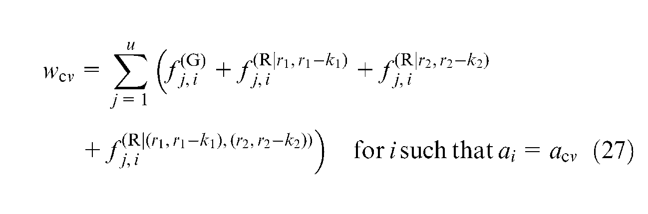
For the common workstation a_c, the input flows are from both lines. Hence, the loading w_c of a_c should be modified as

w_{c} = \sum_{j = 1}^{2} (f_{j, i}^{(G)} + f_{j, i}^{(R | r_{1}, r_{1} - k_{1})} + f_{j, i}^{(R | r_{2}, r_{2} - k_{2})} + f_{j, i}^{(R | (r_{1}, r_{1} - k_{1}), (r_{2}, r_{2} - k_{2}))}) f o r i s u c h t h a t a_{i} = a_{c}

(7)

Reliability evaluation

The reliability evaluation relies on the probability that each workstation can provide sufficient capacity to satisfy w_i. According to the second assumption, the capacity of a_i is a random variable, and thus, the production system is stochastic. Let x_i denote the current capacity of a_i, where x_i takes possible values $0 = x_{i 1} < x_{i 2} < \dots < x_{i c_{i}} = M_{i}$ and c_i denotes number of possible capacities of a_i. Under the state $X = (x_{1}, x_{2}, \dots, x_{n_{1} + n_{2}})$ , constraint (8) guarantees that a_i can process the input raw materials/WIP

x_{i} \geq w_{i}, i = 1, 2, \dots, n_{1} + n_{2}

(8)

The state x_i satisfying w_i indicates that a_i provides a sufficient capacity.

Given the demand d, the reliability R(d) is the probability that output products from the CFPN are not less than d. That is, the reliability is Pr{X|V(X) ≥d}, where V(X) is defined as the maximum output under X. However, it is computationally inefficient to find all X such that V(X) ≥d and then accumulate their probabilities to obtain R(d). A capacity vector Y is minimal for d if and only if (a) V(Y) ≥d and (b) V(X) < d for any capacity vector X such that X < Y. Given {Y₁, Y₂, …, Y_h}, the set of minimal capacity vectors capable of satisfying demand d, the reliability R(d) is

R (d) = Pr {⋃_{v = 1}^{h} Ω_{v}}

(9)

where Ω_v = {X|X≥Y_v}, v = 1, 2, …, h. Two algorithms, including a general algorithm, to generate all minimal capacity vectors are proposed in the following subsections.

Algorithm for two lines

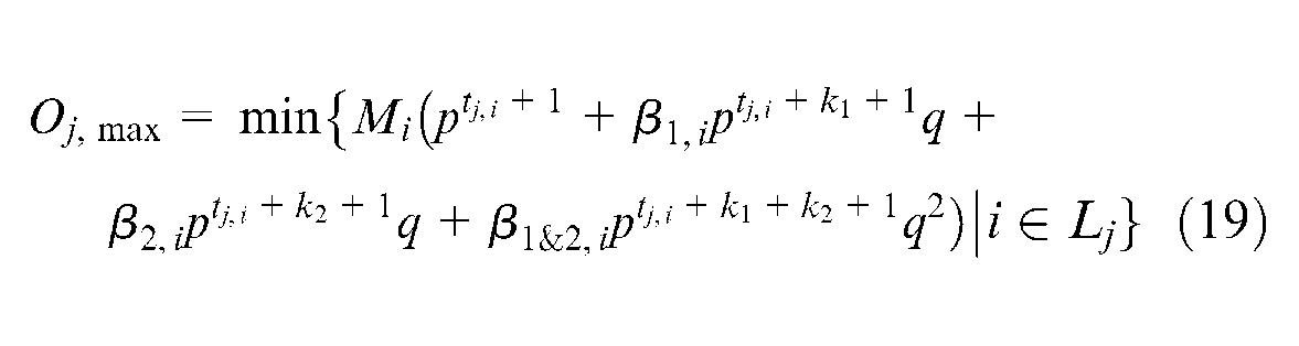
Given two lines L₁ and L₂ with a common workstation a_c (assumed a_c is layout in L₁) in which $L_{1} = {a_{1}, a_{2}, \dots, a_{c}, \dots, a_{n_{1}}}$ and $L_{2} = {a_{n_{1} + 1}, a_{n_{1} + 2}, \dots, a_{c} \dots, a_{n_{1} + n_{2}}}$ . Defective WIP output from r₁th (resp. r₂th) ordered workstation is reworked starting from previous k₁ (resp. k₂) workstations. The minimal capacity vectors for d are generated with the following steps.

Step 1. Find the maximum output for each path

O_{j, max} = min {M_{i} (p^{t_{j, i} + 1} + β_{1, i} p^{t_{j, i} + k_{1} + 1} q + β_{2, i} p^{t_{j, i} + k_{2} + 1} q + β_{1 & 2, i} p^{t_{j, i} + k_{1} + k_{2} + 1} q^{2}) | i \in L_{j}}

(10)

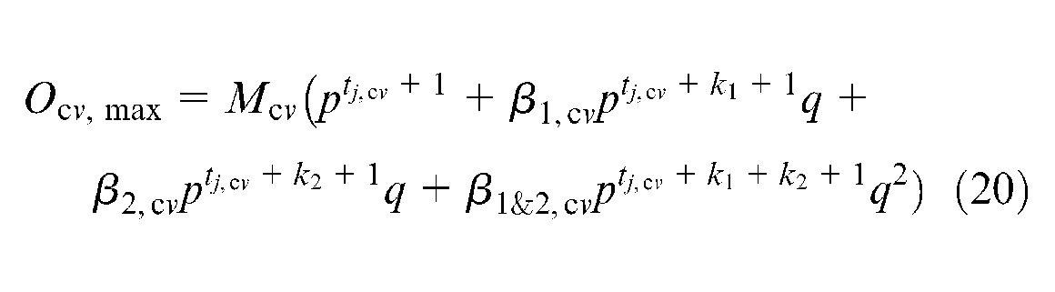
where t_j,_i is the number of follow-up workstations after a_i on $L_{j}^{(G)}$ . The index β_1,i (resp. β_2,i and β_1&2,i) equals 1 for a_i not on $L_{j}^{(R | r_{1}, r_{1} - k_{1})}$ (resp. $L_{j}^{(R | r_{2}, r_{2} - k_{2})}$ and $L_{j}^{(R | (r_{1}, r_{1} - k_{1}), (r_{2}, r_{2} - k_{2}))}$ ); otherwise β_1,i (resp. β_2,i and β_1&2,i) equals 0.

Step 2. Find the maximum output of the common workstation a_c

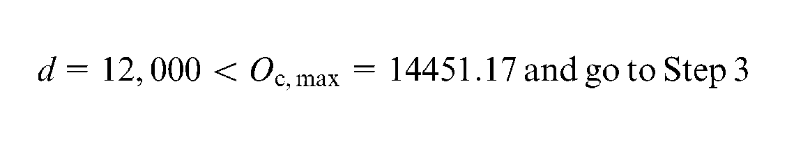
O_{c, max} = M_{c} (p^{t_{j, c} + 1} + β_{1, c} p^{t_{j, c} + k_{1} + 1} q + β_{2, c} p^{t_{j, c} + k_{2} + 1} q + β_{1 & 2, c} p^{t_{j, c} + k_{1} + k_{2} + 1} q^{2})

(11)

If d≤O_c,max, go to Step 3; otherwise, stop (i.e. d > O_c,max indicates that the CFPN cannot satisfy such a demand level).

Step 3. Find the demand assignment (d₁, d₂) satisfying d₁+d₂ = d under constraint d_j≤O_j,_max.

Step 4. For each demand pair (d₁, d₂), do the following steps:

Step 4.1. Determine the amount of input materials for each line by

I_{j} = \frac{d_{j}}{η_{j}}

(12)

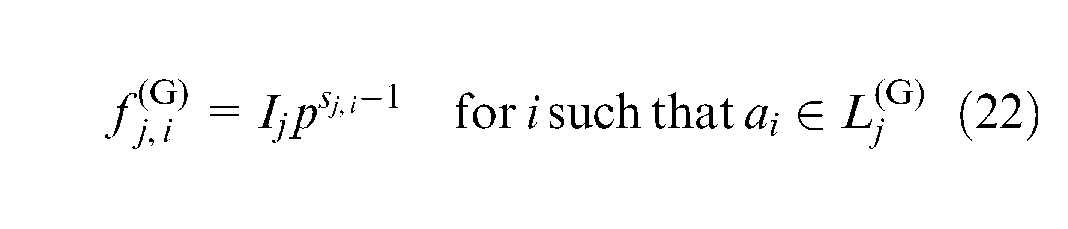
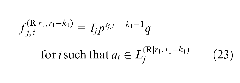
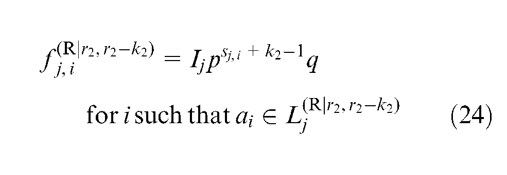
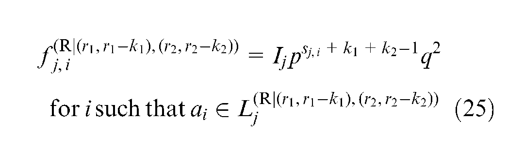
Step 4.2. Determine the input flows for each workstation a_i. For a_i∈L_j, the input flows are derived as follows

f_{j, i}^{(G)} = I_{j} p^{s_{j, i} - 1} for i such that a_{i} \in L_{j}^{(G)}

(13)

f_{j, i}^{(R | r_{1}, r_{1} - k_{1})} = I_{j} p^{s_{j, i} + k_{1} - 1} q for i such that a_{i} \in L_{j}^{(R | r_{1}, r_{1} - k_{1})}

(14)

f_{j, i}^{(R | r_{2}, r_{2} - k_{2})} = I_{j} p^{s_{j, i} + k_{2} - 1} q for i such that a_{i} \in L_{j}^{(R | r_{2}, r_{2} - k_{2})}

(15)

f_{j, i}^{(R | (r_{1}, r_{1} - k_{1}), (r_{2}, r_{2} - k_{2}))} = I_{j} p^{s_{j, i} + k_{1} + k_{2} - 1} q^{2} for i such that a_{i} \in L_{j}^{(R | (r_{1}, r_{1} - k_{1}), (r_{2}, r_{2} - k_{2}))}

(16)

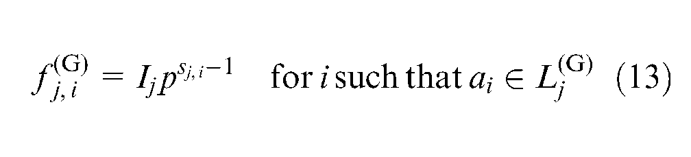
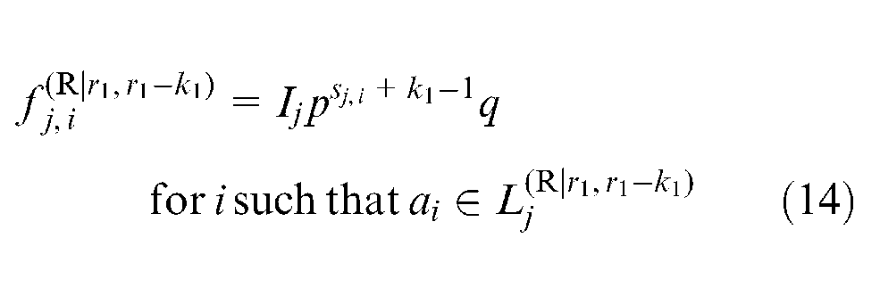
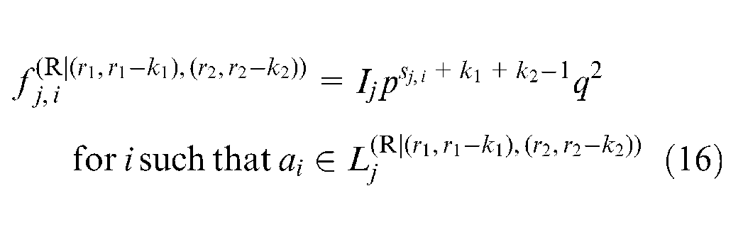
where s_j,_i is the order of a_i on the general production path $L_{j}^{(G)}$ .

Step 4.3. Transform input flows from general production paths and reworking paths into workstations’ loading vector $W = (w_{1}, w_{2}, \dots, w_{n_{1} + n_{2}})$ via

w_{i} = f_{j, i}^{(G)} + f_{j, i}^{(R | r_{1}, r_{1} - k_{1})} + f_{j, i}^{(R | r_{2}, r_{2} - k_{2})} + f_{j, i}^{(R | (r_{1}, r_{1} - k_{1}), (r_{2}, r_{2} - k_{2}))} for i such that a_{i} \in L_{j}

(17)

w_{c} = \sum_{j = 1}^{2} (f_{j, i}^{(G)} + f_{j, i}^{(R | r_{1}, r_{1} - k_{1})} + f_{j, i}^{(R | r_{2}, r_{2} - k_{2})} + f_{j, i}^{(R | (r_{1}, r_{1} - k_{1}), (r_{2}, r_{2} - k_{2}))}) for i such that a_{i} = a_{c}

(18)

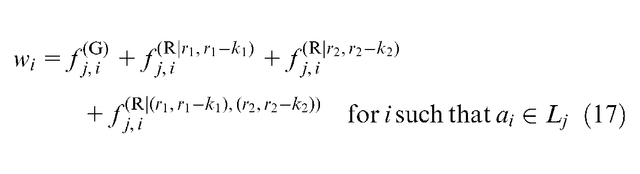
Step 4.4. For each workstation a_i, find the smallest possible capacity x_ic such that $x_{ic} \geq w_{i} > x_{i (c - 1)}$ . Then, $Y = (y_{1}, y_{2}, \dots, y_{n_{1} + n_{2}})$ is a minimal capacity vector for d where y_i = x_ic for all i.

Step 5. Those Y obtained from Step 4 are the minimal capacity vectors for d.

Several methods may be applied to compute the reliability by equation (9), such as inclusion–exclusion method,^7,17,18 state-space decomposition,^19,20 and recursive sum of disjoint products (RSDP) algorithm.^3,6,10 In practice, the RSDP algorithm demonstrates better computational efficiency than the other methods.¹⁰ Hence, the RSDP algorithm is selected as the method to derive reliability herein.

Despite this article considers the same success rate p, the proposed models can be easily extended to the case of each workstation that possesses a distinct success rate. That is, we can replace the same success rate p by a distinct success rate p_i of a_i. For instance, input I₁ units of raw material in L₁, the products produced by $L_{1}^{(G)}$ through workstations $a_{1}, a_{2}, \dots, a_{n_{1}}$ are I₁ $Π_{t = 1}^{n_{1}} p_{t}$ .

General algorithm for multiple lines

This section further addresses an extension case of more than two lines and more than one common workstation. A general algorithm is proposed to deal with CFPN with multiple lines. Given u lines, say L₁, L₂, …, L_u, in a CFPN and each line L_j consists of n_j workstations, where j = 1, 2, …, u. When producing the same product type, m workstations, say a_c1, a_c2, …, a_cm, are utilized as common workstations. For each line, defective WIP output from r₁th (resp. r₂th) ordered workstation is reworked starting from previous k₁ (resp. k₂) workstations. The minimal capacity vectors for d are generated with the following steps:

Step 1. Find the maximum output for each path

O_{j, \max} = \min {M_{i} (p^{t_{j, i} + 1} + β_{1, i} p^{t_{j, i} + k_{1} + 1} q + β_{2, i} p^{t_{j, i} + k_{2} + 1} q + β_{1 & 2, i} p^{t_{j, i} + k_{1} + k_{2} + 1} q^{2}) | i \in L_{j}}

(19)

Step 2. Find the maximum output O_cv,max of the vth common workstation a_cv, where v = 1, 2, …, m

O_{c v, max} = M_{c v} (p^{t_{j, c v} + 1} + β_{1, c v} p^{t_{j, c v} + k_{1} + 1} q + β_{2, c v} p^{t_{j, c v} + k_{2} + 1} q + β_{1 & 2, c v} p^{t_{j, c v} + k_{1} + k_{2} + 1} q^{2})

(20)

Step 3. Find the demand assignment (d₁, d₂, …, d_u) satisfying $\sum_{j = 1}^{u} d_{j} = d$ under constraints d_j≤O_j,_max.

Step 4. For each demand assignment (d₁, d₂, …, d_u), do the following steps.

Step 4.1. Determine the amount of input materials for each line by

I_{j} = \frac{d_{j}}{η_{j}}

(21)

Step 4.2. Determine the input flows for each workstation a_i. For a_i∈L_j, the input flows are derived as follows

f_{j, i}^{(G)} = I_{j} p^{s_{j, i} - 1} for i such that a_{i} \in L_{j}^{(G)}

(22)

f_{j, i}^{(R | r_{1}, r_{1} - k_{1})} = I_{j} p^{s_{j, i} + k_{1} - 1} q for i such that a_{i} \in L_{j}^{(R | r_{1}, r_{1} - k_{1})}

(23)

f_{j, i}^{(R | r_{2}, r_{2} - k_{2})} = I_{j} p^{s_{j, i} + k_{2} - 1} q for i such that a_{i} \in L_{j}^{(R | r_{2}, r_{2} - k_{2})}

(24)

f_{j, i}^{(R | (r_{1}, r_{1} - k_{1}), (r_{2}, r_{2} - k_{2}))} = I_{j} p^{s_{j, i} + k_{1} + k_{2} - 1} q^{2} for i such that a_{i} \in L_{j}^{(R | (r_{1}, r_{1} - k_{1}), (r_{2}, r_{2} - k_{2}))}

(25)

Step 4.3. Transform input flows from general production paths and reworking paths into workstations’ loading vector $W = (w_{1}, w_{2}, \dots, w_{n_{1} + n_{2} + \dots + n_{u}})$ via

w_{i} = f_{j, i}^{(G)} + f_{j, i}^{(R | r_{1}, r_{1} - k_{1})} + f_{j, i}^{(R | r_{2}, r_{2} - k_{2})} + f_{j, i}^{(R | (r_{1}, r_{1} - k_{1}), (r_{2}, r_{2} - k_{2}))} for i such that a_{i} \in L_{j}

(26)

w_{c v} = \sum_{j = 1}^{u} (f_{j, i}^{(G)} + f_{j, i}^{(R | r_{1}, r_{1} - k_{1})} + f_{j, i}^{(R | r_{2}, r_{2} - k_{2})} + f_{j, i}^{(R | (r_{1}, r_{1} - k_{1}), (r_{2}, r_{2} - k_{2}))}) for i such that a_{i} = a_{c v}

(27)

Step 4.4. For each workstation a_i, find the smallest possible capacity x_ic such that $x_{ic} \geq w_{i} > x_{i (c - 1)}$ . Then, $Y = (y_{1}, y_{2}, \dots, y_{n_{1} + n_{2} + \dots + n_{u}})$ is a minimal capacity vector for d where y_i = x_ic for all i.

Step 5. Those Y obtained from Step 4 are the minimal capacity vectors for d.

Case study

In this section, a PCB production system is utilized to demonstrate the reliability evaluation procedure. The PCB production system consists of two lines (u = 2) and one common workstation (m = 1), which can be mapped into Figure 1.

PCB production process

For the single-sided board production, the input raw material is a board with a thin layer of copper foil. Generally, the regular production process of a PCB is starting from shearing workstations (a₁, a₁₁) in which the board is cut as a specific size. Subsequently, automated drilling workstations (a₂, a₁₂) drill holes through the board for mounting electronic components on it. After drilling, the deburring workstations (a₃, a₁₃) remove copper particles from the board and then the scrubbing workstations (a₄, a₁₄) are responsible for cleaning the board. Electroless copper plating workstations ( a ₅ ) are subsequently employed to provide a thin conductive layer over the surface of the board. Note that a ₅ is set to be the common workstation to share its capacity for both lines. Following electroless copper plating, the photo imaging workstations (a₆, a₁₅) create the circuit pattern on the board. By chemical etching (a₇, a₁₆) and resist stripping (a₈, a₁₇), the copper not part of the circuit pattern is removed. Once again, scrubbing workstations (a₉, a₁₈) are for cleaning the chemicals and resist on the board. Finally, the legend printing workstations (a₁₀, a₁₉) put the required logos or letters on the boards. In such a PCB production process, the first reworking action is that defective WIP output from a₃ (resp. a₁₃) reworked by the original workstation a₃ (resp. a₁₃), while the second reworking action is that defective WIP output from a₉ (resp. a₁₈) reworked starting from a₇ (resp. a₁₆). The above-mentioned PCB production system with two lines and a common workstation can be mapped into Figure 1. Thus, the transformed CFPN and the decomposed paths are shown in Figures 2 and 3, respectively.

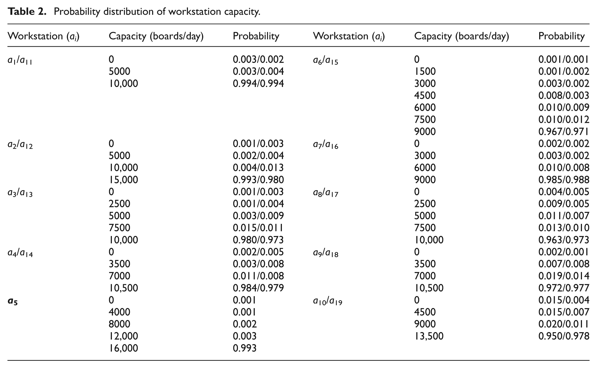
The capacity of each workstation is measured in number of boards processed per day (boards/day). For instance, the specification of a deburring machine is estimated as 300,000 ft²/month. That is, for the board size of 24″×24″, the capacity of the deburring machine is 75,000 boards/month (i.e. 2500 boards/day). A deburring workstation comprising four machines possesses five capacity states, say 0, 2500, 5000, 7500, and 10,000 (boards/day). The lowest level 0 corresponds to complete malfunction of all machines, while 10,000 will be the highest level when all machines operate successfully.

Reliability evaluation

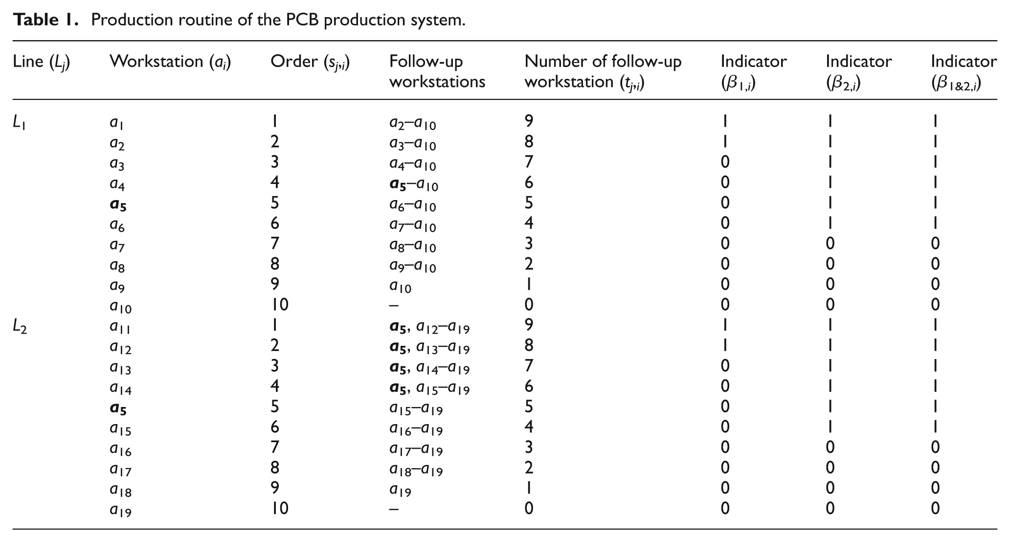
Production routine of PCB production system is provided in Table 1. The capacity distribution of workstation in Table 2 is in the form of probability mass function, indicating that each workstation can provide a certain capacity level with a corresponding probability. For instance, the probability of workstation a ₅ can produce 12,000 boards/day (or more) is Pr{x₅≥ 12,000} = Pr{x₅ = 12,000} + Pr{x₅ = 16,000} = 0.003 + 0.993 = 0.996.

Table 1.

Production routine of the PCB production system.

Line (L_j)	Workstation (a_i)	Order (s_j,_i)	Follow-up workstations	Number of follow-up workstation (t_j,_i)	Indicator (β_1,i)	Indicator (β_2,i)	Indicator (β_1&2,i)
L ₁	a ₁	1	a₂–a₁₀	9	1	1	1
	a ₂	2	a₃–a₁₀	8	1	1	1
	a ₃	3	a₄–a₁₀	7	0	1	1
	a ₄	4	a ₅ –a₁₀	6	0	1	1
	a ₅	5	a₆–a₁₀	5	0	1	1
	a ₆	6	a₇–a₁₀	4	0	1	1
	a ₇	7	a₈–a₁₀	3	0	0	0
	a ₈	8	a₉–a₁₀	2	0	0	0
	a ₉	9	a ₁₀	1	0	0	0
	a ₁₀	10	–	0	0	0	0
L ₂	a ₁₁	1	a ₅ , a₁₂–a₁₉	9	1	1	1
	a ₁₂	2	a ₅ , a₁₃–a₁₉	8	1	1	1
	a ₁₃	3	a ₅ , a₁₄–a₁₉	7	0	1	1
	a ₁₄	4	a ₅ , a₁₅–a₁₉	6	0	1	1
	a ₅	5	a₁₅–a₁₉	5	0	1	1
	a ₁₅	6	a₁₆–a₁₉	4	0	1	1
	a ₁₆	7	a₁₇–a₁₉	3	0	0	0
	a ₁₇	8	a₁₈–a₁₉	2	0	0	0
	a ₁₈	9	a ₁₉	1	0	0	0
	a ₁₉	10	–	0	0	0	0

Table 2.

Probability distribution of workstation capacity.

Workstation (a_i)	Capacity (boards/day)	Probability	Workstation (a_i)	Capacity (boards/day)	Probability
a₁/a₁₁	0	0.003/0.002	a₆/a₁₅	0	0.001/0.001
	5000	0.003/0.004		1500	0.001/0.002
	10,000	0.994/0.994		3000	0.003/0.002
				4500	0.008/0.003
				6000	0.010/0.009
				7500	0.010/0.012
				9000	0.967/0.971
a₂/a₁₂	0	0.001/0.003	a₇/a₁₆	0	0.002/0.002
	5000	0.002/0.004		3000	0.003/0.002
	10,000	0.004/0.013		6000	0.010/0.008
	15,000	0.993/0.980		9000	0.985/0.988
a₃/a₁₃	0	0.001/0.003	a₈/a₁₇	0	0.004/0.005
	2500	0.001/0.004		2500	0.009/0.005
	5000	0.003/0.009		5000	0.011/0.007
	7500	0.015/0.011		7500	0.013/0.010
	10,000	0.980/0.973		10,000	0.963/0.973
a₄/a₁₄	0	0.002/0.005	a₉/a₁₈	0	0.002/0.001
	3500	0.003/0.008		3500	0.007/0.008
	7000	0.011/0.008		7000	0.019/0.014
	10,500	0.984/0.979		10,500	0.972/0.977
a ₅	0	0.001	a₁₀/a₁₉	0	0.015/0.004
	4000	0.001		4500	0.015/0.007
	8000	0.002		9000	0.020/0.011
	12,000	0.003		13,500	0.950/0.978
	16,000	0.993

Suppose that the PCB production system has to satisfy the demand d = 12,000 (boards/day) in which output boards are batched by every 1000 units. Given a success rate p = 0.98, the reliability R(12,000) is derived with the following steps:

Step 1. Find the maximum output for each path

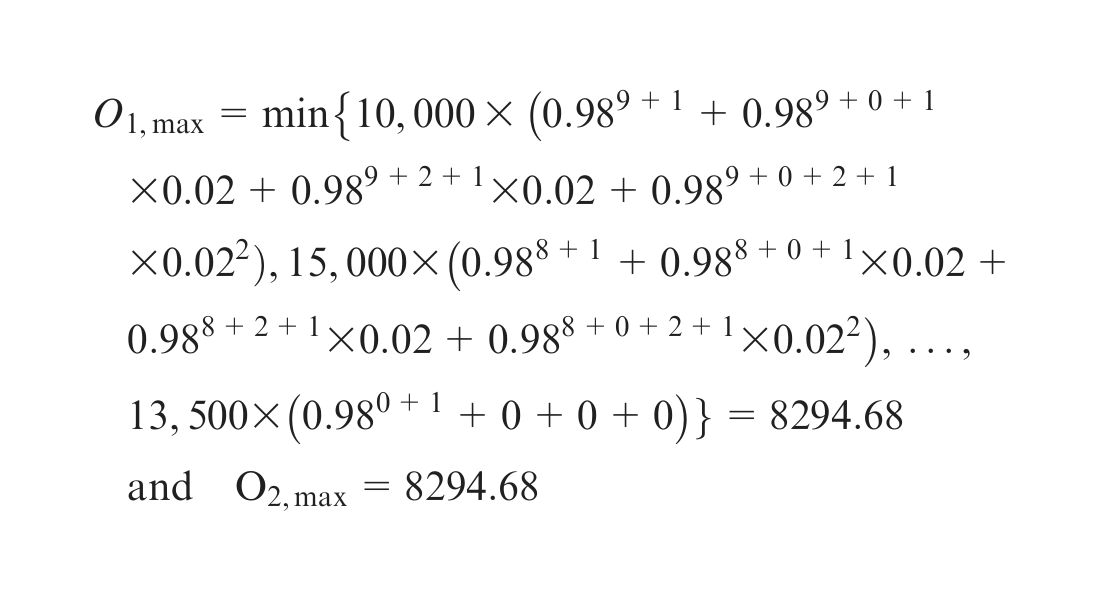
\begin{matrix} O_{1, max} = min {10, 000 \times (0.9 8^{9 + 1} + {0.98}^{9 + 0 + 1} \times 0.02 + 0.9 8^{9 + 2 + 1} \times 0.02 + 0.9 8^{9 + 0 + 2 + 1} \times 0.0 2^{2}), 15, 000 \times (0.9 8^{8 + 1} + 0.9 8^{8 + 0 + 1} \times 0.02 + \\ 0.9 8^{8 + 2 + 1} \times 0.02 + 0.9 8^{8 + 0 + 2 + 1} \times 0.0 2^{2}), \dots, 13, 500 \times (0.9 8^{0 + 1} + 0 + 0 + 0)} = 8294.68 and O_{2, max} = 8294.68 \end{matrix}

Step 2. Find the maximum output of the common workstation a_c

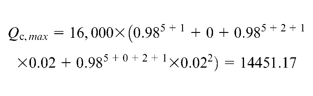
Q_{c, \max} = 16, 000 \times (0.9 8^{5 + 1} + 0 + 0.9 8^{5 + 2 + 1} \times 0.02 + 0.9 8^{5 + 0 + 2 + 1} \times 0.0 2^{2}) = 14451.17

d = 12, 000 < O_{c, max} = 14451.17 and go to Step 3

Step 3. Find the demand assignment (d₁, d₂) satisfying d₁+d₂ = 12,000 under constraints d₁≤ 8294.68 and d₂≤ 8294.68. Since the output boards are batched by every 1000 units, the feasible demand pairs are D₁ = (8000, 4000), D₂ = (7000, 5000), D₃ = (6000, 6000), D₄ = (5000, 7000), and D₅ = (4000, 8000).

Step 4. For each demand pair (d₁, d₂), do the following steps:

(a) For D₁ = (8000, 4000)

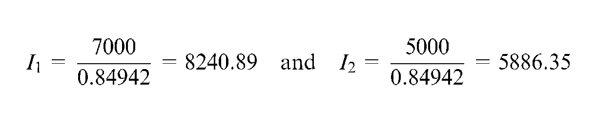
Step 4.1a. Determine the amount of input materials for each line by

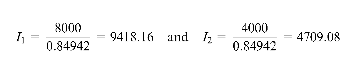
I_{1} = \frac{8000}{0.84942} = 9418.16 a n d I_{2} = \frac{4000}{0.84942} = 4709.08

where the overall success rate of L₁ is $η_{1} = (p^{n} + p^{n + k_{1}} q + p^{n + k_{2}} q + p^{n + k_{1} + k_{2}} q^{2}) = 0.9 8^{10} + 0.9 8^{10 + 0} \times 0.02 + 0.9 8^{10 + 2} \times 0.02 + 0.9 8^{10 + 0 + 2} \times 0.0 2^{2} = 0.84942$ .

Table 3.

Results of Step 4 for (d₁, d₂) = (8000, 4000).

	a ₁	a ₂	a ₃	a ₄	a ₅	a ₆	a ₇	a ₈	a ₉	a ₁₀
$f_{1, i}^{(G)}$	9418.16	9229.80	9045.20	8864.30	8687.01	8513.27	8343.01	8176.15	8012.63	7852.37
$f_{1, i}^{(R \| 3, 3)}$	0.00	0.00	180.90	177.29	173.74	170.27	166.86	163.52	160.25	157.05
$f_{1, i}^{(R \| 8, 6)}$	0.00	0.00	0.00	0.00	0.00	0.00	160.25	157.05	153.91	150.83
$f_{1, i}^{(R \| (3, 3), (8, 6))}$	0.00	0.00	0.00	0.00	0.00	0.00	3.21	3.14	3.08	3.02
w_i	9418.16	9229.80	9226.11	9041.59	8860.75	8683.54	8673.33	8499.86	8329.86	8163.27
y_i	10,000	10,000	10,000	10,500	−^a	9000	9000	10,000	10,500	9000
	a ₁₁	a ₁₂	a ₁₃	a ₁₄	a ₅	a ₁₅	a ₁₆	a ₁₇	a ₁₈	a ₁₉
$f_{2, i}^{(G)}$	4709.08	4614.90	4522.60	4432.15	4343.51	4256.64	4171.50	4088.07	4006.31	3926.19
$f_{2, i}^{(R \| 3, 3)}$	0.00	0.00	90.45	88.64	86.87	85.13	83.43	81.76	80.13	78.52
$f_{2, i}^{(R \| 8, 6)}$	0.00	0.00	0.00	0.00	0.00	0.00	80.13	78.52	76.95	75.41
$f_{2, i}^{(R \| (3, 3), (8, 6))}$	0.00	0.00	0.00	0.00	0.00	0.00	1.60	1.57	1.54	1.51
w_i	4709.08	4614.90	4613.05	4520.79	4430.38	4341.77	4336.66	4249.93	4164.93	4081.63
y_i	5000	5000	5000	7000	−^a	4500	6000	5000	7000	4500

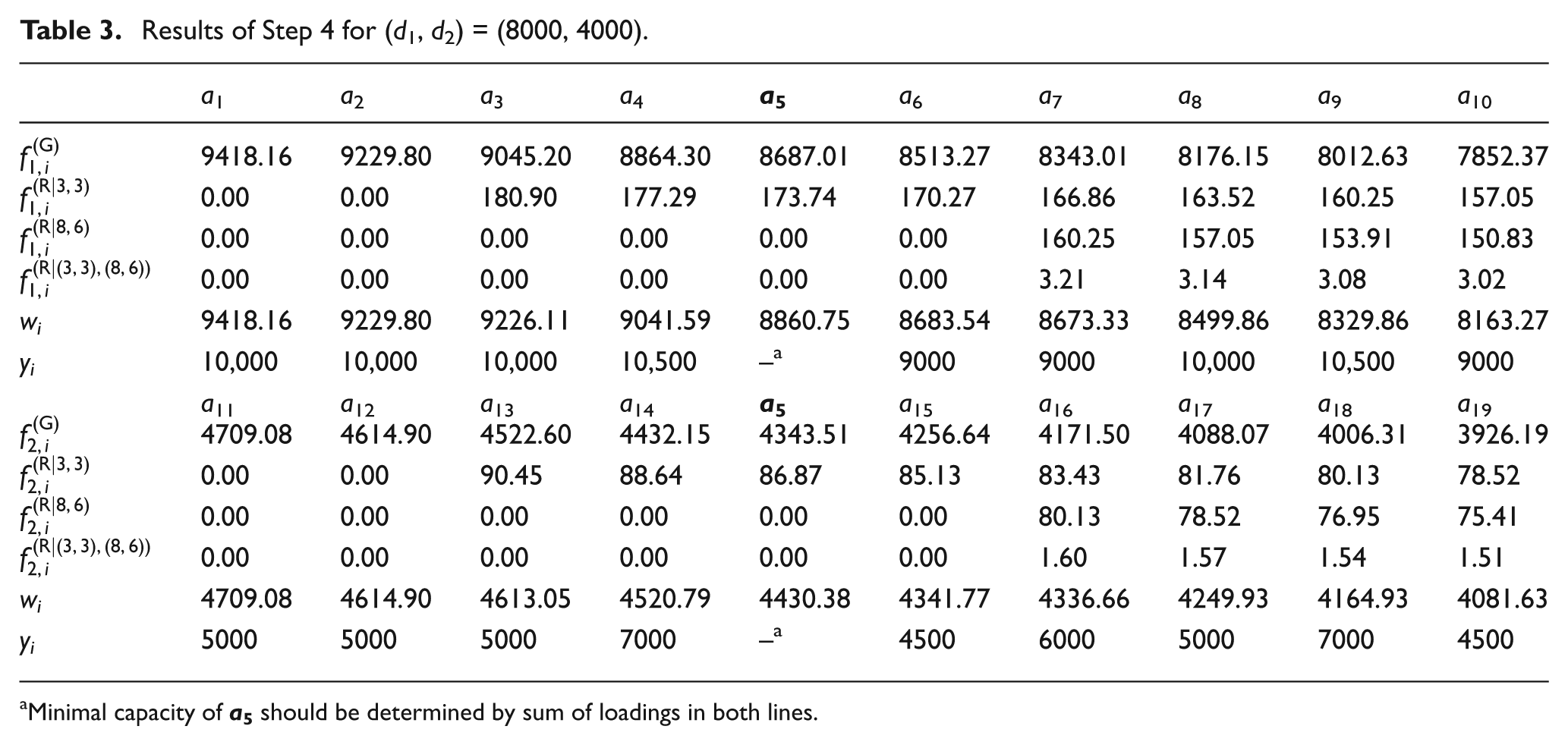
Minimal capacity of a ₅ should be determined by sum of loadings in both lines.

Step 4.2a. For demand pair D₁ = (8000, 4000), the input flow of each workstation is shown in Table 3 (see the row of f_j,_i).

Step 4.3a. Transform input flows from both general production path and reworking paths into the workstations’ loading vector W₁ = (9418.16, 9229.80, 9226.11, 9041.59, 8860.75+4430.38, 8683.54, 8673.33, 8499.86, 8329.86, 8163.27, 4709.08, 4614.90, 4613.05, 4520.79, 4341.77, 4336.66, 4249.93, 4164.93, 4081.63). The calculation of common workstation is italicized. The calculation process is summarized in Table 3 (see the row of w_i).

Step 4.4a. For demand pair D₁ = (8000, 4000), the minimal capacity vector Y₁ = (10,000, 10,000, 10,000, 10,500, 16,000, 9000, 9000, 10,000, 10,500, 9000, 5000, 5000, 5000, 7000, 4500, 6000, 5000, 7000, 4500). The calculation process is summarized in Table 3 (see the row of y_i).

(b) For D₂ = (7000, 5000)

Step 4.1b. Determine the amount of input materials for each line by

I_{1} = \frac{7000}{0.84942} = 8240.89 a n d I_{2} = \frac{5000}{0.84942} = 5886.35

$⋮$

Step 5. Five minimal capacity vectors for d = 12,000 are obtained from Step 4. The results are summarized in Table 4.

Table 4.

Minimal capacity vectors generated.

Demand pair	Minimal capacity vector
D₁ = (8000, 4000)	Y₁ = (10,000, 10,000, 10,000, 10,500, 16,000, 9000, 9000, 10,000, 10,500, 9000, 5000, 5000, 5000, 7000, 4500, 6000, 5000, 7000, 4500)
D₂ = (7000, 5000)	Y₂ = (10,000, 10,000, 10,000, 10,500, 16,000, 9000, 9000, 7500, 10,500, 9000, 10,000, 10,000, 7500, 7000, 6000, 6000, 7500, 7000, 9000)
D₃ = (6000, 6000)	Y₃ = (10,000, 10,000, 5000, 7000, 16,000, 7500, 9000, 7500, 7000, 9000, 10,000, 10,000, 7500, 7000, 7500, 9000, 7500, 7000, 9000)
D₄ = (5000, 7000)	Y₄ = (10,000, 10,000, 7500, 7000, 16,000, 6000, 6000, 7500, 7000, 9000, 10,000, 10,000, 10,000, 10,500, 9000, 9000, 7500, 10,500, 9000)
D₅ = (4000, 8000)	Y₅ = (5000, 5000, 5000, 7000, 16,000, 4500, 6000, 5000, 7000, 4500, 10,000, 10,000, 10,000, 10,500, 9000, 9000, 10,000, 10,500, 9000)

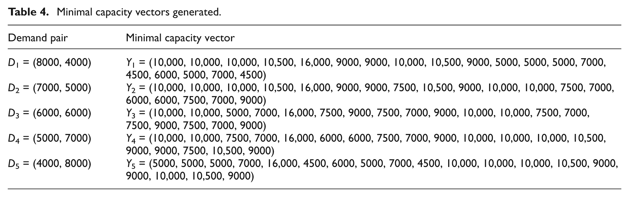
After obtaining all minimal capacity vectors for d = 12,000, we suppose that Ω₁ = {X|X≥Y₁}, Ω₂ = {X|X≥Y₁}, …, and Ω₅ = {X|X≥Y₅}. The reliability R(12,000) = Pr{Ω₁∪Ω₂∪Ω₃∪Ω₄∪Ω₅} = 0.87670 is derived by the RSDP algorithm. It means that the PCB production system can produce 12,000 boards/day with a probability of 0.87670.

Conclusion and future research

To evaluate the reliability for a more practical production system, this article modified the previous work,³ which was proposed only for parallel-line production systems without common workstation, to the case of intersectional lines and multiple reworking actions. The performance evaluation process is summarized as a three-phase flow chart, as shown in Figure 4. In the model construction phase, the production system is constructed as a network-structured CFPN by revised transformation and decomposition techniques. This CFPN is beneficial for the capacity analysis phase, such as determinations of input raw materials, maximum output of each line, and input flow of each workstation. In particular, the proposed techniques can deal with the common workstation whose input flows are from different lines. In the phase of minimal capacity vector generation, two simple algorithms are developed to generate all minimal capacity vectors that workstations should provide to satisfy demand d. In terms of such vectors, the reliability is evaluated in the third phase. According to the reliability, the production manager could conduct a sensitivity analysis to investigate the most important workstation in the CFPN to improve the reliability. The production manager can find the most sensitive workstation that decreases the reliability most, and such a workstation is the most important part of the CFPN.

Figure 4.

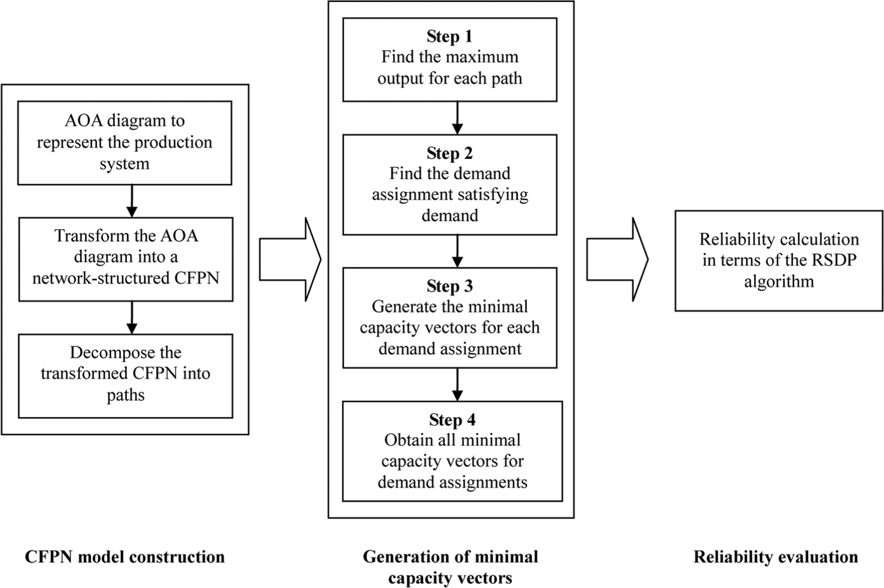
Procedure to evaluate the reliability.

The limitation of the proposed methodology is that we primarily focus on two reworking actions at each line. When adopting the proposed methodology, the topology will become very complex if there are many reworking actions. For instance, there are eight decomposed paths for three reworking actions, including one general production path, three single-reworking paths, three double-reworking paths, and one triple reworking path. Future research may pursue an estimation method for the case of more than two reworking actions. Theoretically, the proposed methodology in this article is possible to deal with the case of more than two reworking actions once all the decomposed paths are obtained. However, it is very complicated to develop a general model, and hence, an estimation method should be developed in the future.

Footnotes

Appendix 1 Declaration of conflicting interests

The authors declare that there is no conflict of interest.

Funding

This work was supported in part by the National Science Council, Taiwan, Republic of China, under Grant No. NSC 99-2221-E-011-066-MY3.

References

Chen

Lan

. The maximal profit flow model in designing multiple-production-line system with obtainable resource capacity. Int J Prod Econ 2001; 70: 175–184.

Lan

. The design of multiple production lines under deadline constraint. Int J Prod Econ 2007; 106: 191–203.

Lin

Chang

Chen

. Reliability evaluation for a waste-reduction parallel-line manufacturing system. J Clean Prod 2012; 35: 93–101.

Lin

Jane

Yuan

. On reliability evaluation of a capacitated-flow network in terms of minimal pathsets. Networks 1995; 25: 131–138.

Lin

. On transmission time through k minimal paths of a capacitated-flow network. Appl Math Model 2010; 34: 245–253.

Lin

Chang

. Evaluation of system reliability for a cloud computing system with imperfect nodes. Syst Eng 2012; 15: 83–94.

Lin

. Two-commodity reliability evaluation of a stochastic-flow network with varying capacity weight in terms of minimal paths. Comput Oper Res 2009; 36: 1050–1063.

Yeh

. A simple minimal path method for estimating the weighted multi-commodity multistate unreliable networks reliability. Reliab Eng Syst Safe 2008; 93: 125–136.

Yeh

. A sequential decomposition method for estimating flow in a multi-commodity, multistate network. IEEE T Reliab 2011; 60: 612–621.

10.

Zuo

Tian

Huang

. An efficient method for reliability evaluation of multistate networks given all minimal path vectors. IIE Trans 2007; 39: 811–817.

11.

Lin

. On performance evaluation for a multistate network under spare routing. Inform Sciences 2012; 203: 73–82.

12.

Ford

Fulkerson

. Flows in network. Princeton, NJ: Princeton University Press, 1962.

13.

Chiu

YSP

Tseng

Ting

. Economic manufacturing quantity model with imperfect rework and random breakdown under. Proc IMechE, Part B: J Engineering Manufacture 2009; 223: 183–194.

14.

Leung

KNF

. Optimal production lot sizing with backlogging, random defective rate, and rework derived without derivatives. Proc IMechE, Part B: J Engineering Manufacture 2009; 223: 1081–1084.

15.

Buscher

Lindner

. Optimizing a production system with rework and equal sized batch shipment. Comput Oper Res 2007; 34: 515–535.

16.

Teunter

Kaparis

Tang

. Multi-product economic lot scheduling problem with separate production lines for manufacturing and remanufacturing. Eur J Oper Res 2008; 191: 1241–1253.

17.

Hudson

Kapur

. Reliability bounds for multistate systems with multistate components. Oper Res 1985; 33: 153–160.

18.

Xue

. On multistate system analysis. IEEE T Reliab 1985; 34: 329–337.

19.

Aven

. Reliability evaluation of multistate systems with multistate components. IEEE T Reliab 1985; 34: 473–479.

20.

Alexopoulos

. A note on state-space decomposition methods for analyzing stochastic flow networks. IEEE T Reliab 1995; 44: 354–357.

Reliability of a production system with intersectional lines

Abstract

Keywords

Introduction

Model building

AOA-formed representation

Revised transformation and decomposition techniques

Flow analysis and reliability

Input flow analysis

Reliability evaluation

Algorithm for two lines

General algorithm for multiple lines

Case study

PCB production process

Reliability evaluation

Conclusion and future research

Footnotes

Appendix 1

Declaration of conflicting interests

Funding

References